NONLINEAR ACCELERATOR PROBLEMS VIA WAVELETS:
4. SPIN-ORBITAL MOTION

Abstract

In this series of eight papers we present the applications of methods from wavelet analysis to polynomial approximations for a number of accelerator physics problems. In this part we consider a model for spin-orbital motion: orbital dynamics and Thomas-BMT equations for classical spin vector. We represent the solution of this dynamical system in framework of biorthogonal wavelets via variational approach. We consider a different variational approach, which is applied to each scale.

1 INTRODUCTION

This is the fourth part of our eight presentations in which we consider applications of methods from wavelet analysis to nonlinear accelerator physics problems. This is a continuation of our results from [1]-[8], which is based on our approach to investigation of nonlinear problems – general, with additional structures (Hamiltonian, symplectic or quasicomplex), chaotic, quasiclassical, quantum, which are considered in the framework of local (nonlinear) Fourier analysis, or wavelet analysis. Wavelet analysis is a relatively novel set of mathematical methods, which gives us a possibility to work with well-localized bases in functional spaces and with the general type of operators (differential, integral, pseudodifferential) in such bases. In this part we consider spin orbital motion. In section 3 we consider generalization of our approach from part 1 to variational formulation in the biorthogonal bases of compactly supported wavelets. In section 4 we consider the different variational multiresolution approach which gives us possibility for computations in each scale separately.

2 Spin-Orbital Motion

Let us consider the system of equations for orbital motion and Thomas-BMT equation for classical spin vector [9]: $\mathrm{d}q/\mathrm{d}t={\partial H_{orb}}/{\partial p},\quad{\mathrm{d}p}/{\mathrm{d}t}=-{\partial H_{orb}}/{\partial q}$, $\quad\mathrm{d}s/\mathrm{d}t=w\times s$, where

$$H_{orb} = c\sqrt{\pi^{2}+m_{0}c^{2}}+e\Phi,$$

$$w= - \frac{e}{m_{0}c\gamma}(1+\gamma G)\vec{B}$$

$$+ \frac{e}{m_{0}^{3}c^{3}\gamma}\frac{G(\vec{\pi}\cdot\vec{B})\vec{\pi}}{(1+\gamma)}$$

$$+ \frac{e}{m_{0}^{2}c^{2}\gamma}\frac{G+\gamma G+1}{(1+\gamma)}[\pi\times E],$$

$q=(q_{1},q_{2},q_{3}),p=(p_{1},p_{2},p_{3})$ are canonical position and momentum, $s=(s_{1},s_{2},s_{3})$ is the classical spin vector of length $\hbar/2$, $\pi=(\pi_{1},\pi_{2},\pi_{3})$ is kinetic momentum vector. We may introduce in 9-dimensional phase space $z=(q,p,s)$ the Poisson brackets $\{f(z),g(z)\}=f_{q}g_{p}-f_{p}g_{q}+[f_{s}\times g_{s}]\cdot s$ and the Hamiltonian equations are ${\mathrm{d}z}/{\mathrm{d}t}=\{z,H\}$ with Hamiltonian

$$H=H_{orb}(q,p,t)+w(q,p,t)\cdot s.$$ (2)

More explicitly we have

$$\frac{\mathrm{d}q}{\mathrm{d}t} = \frac{\partial H_{orb}}{\partial p}+\frac{\partial(w\cdot s)}{\partial p}$$

$$\frac{\mathrm{d}p}{\mathrm{d}t} = -\frac{\partial H_{orb}}{\partial q}-\frac{\partial(w\cdot s)}{\partial q}$$ (3)

$$\frac{\mathrm{d}s}{\mathrm{d}t} = [w\times s]$$

We will consider this dynamical system also in another paper via invariant approach, based on consideration of Lie-Poison structures on semidirect products. But from the point of view which we used in this paper we may consider the similar approximations as in the preceding parts and then we also arrive to some type of polynomial dynamics.

3 VARIATIONAL APPROACH IN BIORTHOGONAL WAVELET BASES

Because integrand of variational functionals is represented by bilinear form (scalar product) it seems more reasonable to consider wavelet constructions [10] which take into account all advantages of this structure. The action functional for loops in the phase space is [11]

$$F(\gamma)=\displaystyle\int_{\gamma}pdq-\int_{0}^{1}H(t,\gamma(t))dt$$ (4)

The critical points of $F$ are those loops $\gamma$, which solve the Hamiltonian equations associated with the Hamiltonian $H$ and hence are periodic orbits. By the way, all critical points of $F$ are the saddle points of infinite Morse index, but surprisingly this approach is very effective. This will be demonstrated using several variational techniques starting from minimax due to Rabinowitz and ending with Floer homology. So, $(M,\omega)$ is symplectic manifolds, $H:M\to R$, $H$ is Hamiltonian, $X_{H}$ is unique Hamiltonian vector field defined by $\omega(X_{H}(x),\upsilon)=-dH(x)(\upsilon),\quad\upsilon\in T_{x}M,\quad x\in M,$ where $\omega$ is the symplectic structure. A T-periodic solution $x(t)$ of the Hamiltonian equations $\dot{x}=X_{H}(x)$ on M is a solution, satisfying the boundary conditions $x(T)$ $=x(0),T>0$. Let us consider the loop space $\Omega=C^{\infty}(S^{1},R^{2n})$, where $S^{1}=R/{\bf Z}$, of smooth loops in $R^{2n}$. Let us define a function $\Phi:\Omega\to R$ by setting

$$\Phi(x)=\displaystyle\int_{0}^{1}\frac{1}{2}<-J\dot{x},x>dt-\int_{0}^{1}H(x(t))dt,\quad x\in\Omega$$ (5)

The critical points of $\Phi$ are the periodic solutions of $\dot{x}=X_{H}(x)$. Computing the derivative at $x\in\Omega$ in the direction of $y\in\Omega$, we find

$$\Phi^{\prime}(x)(y)=\frac{d}{d\epsilon}\Phi(x+\epsilon y)|_{\epsilon=0}=$$ (6)

$$\displaystyle\int_{0}^{1}<-J\dot{x}-\bigtriangledown H(x),y>dt$$

Consequently, $\Phi^{\prime}(x)(y)=0$ for all $y\in\Omega$ iff the loop $x$ satisfies the equation

$$-J\dot{x}(t)-\bigtriangledown H(x(t))=0,$$ (7)

i.e. $x(t)$ is a solution of the Hamiltonian equations, which also satisfies $x(0)=x(1)$, i.e. periodic of period 1. Periodic loops may be represented by their Fourier series: $x(t)=\sum e^{k2\pi Jt}x_{k},\ x_{k}\in R^{2k}$, where $J$ is quasicomplex structure. We give relations between quasicomplex structure and wavelets in our other paper. But now we need to take into account underlying bilinear structure via wavelets. We started with two hierarchical sequences of approximations spaces [10]:

$$\dots V_{-2}\subset V_{-1}\subset V_{0}\subset V_{1}\subset V_{2}\dots,$$ (8)

$$\dots\widetilde{V}_{-2}\subset\widetilde{V}_{-1}\subset\widetilde{V}_{0}\subset\widetilde{V}_{1}\subset\widetilde{V}_{2}\dots,$$

and as usually, $W_{0}$ is complement to $V_{0}$ in $V_{1}$, but now not necessarily orthogonal complement. New orthogonality conditions have now the following form:

$$\widetilde{W}_{0}\perp V_{0},\quad W_{0}\perp\widetilde{V}_{0},\quad V_{j}\perp\widetilde{W}_{j},\quad\widetilde{V}_{j}\perp W_{j}$$ (9)

translates of $\psi$ $\mathrm{span}$ $W_{0}$, translates of $\tilde{\psi}\quad\mathrm{span}\quad\widetilde{W}_{0}$. Biorthogonality conditions are

$$<\psi_{jk},\tilde{\psi}_{j^{\prime}k^{\prime}}>=\int^{\infty}_{-\infty}\psi_{jk}(x)\tilde{\psi}_{j^{\prime}k^{\prime}}(x)\mathrm{d}x=\delta_{kk^{\prime}}\delta_{jj^{\prime}},$$ (10)

where $\psi_{jk}(x)=2^{j/2}\psi(2^{j}x-k)$. Functions $\varphi(x),\tilde{\varphi}(x-k)$ form dual pair: $<\varphi(x-k),\tilde{\varphi}(x-\ell)>=\delta_{kl}$, $<\varphi(x-k),\tilde{\psi}(x-\ell)>=0$. Functions $\varphi,\tilde{\varphi}$ generate a multiresolution analysis. $\varphi(x-k)$, $\psi(x-k)$ are synthesis functions, $\tilde{\varphi}(x-\ell)$, $\tilde{\psi}(x-\ell)$ are analysis functions. Synthesis functions are biorthogonal to analysis functions. Scaling spaces are orthogonal to dual wavelet spaces. Two multiresolutions are intertwining $V_{j}+W_{j}=V_{j+1},\quad\widetilde{V}_{j}+\widetilde{W}_{j}=\widetilde{V}_{j+1}$. These are direct sums but not orthogonal sums.

So, our representation for solution has now the form

$$f(t)=\sum_{j,k}\tilde{b}_{jk}\psi_{jk}(t),$$ (11)

where synthesis wavelets are used to synthesize the function. But $\tilde{b}_{jk}$ come from inner products with analysis wavelets. Biorthogonality yields

$$\tilde{b}_{\ell m}=\int f(t)\tilde{\psi}_{\ell m}(t)\mathrm{d}t.$$ (12)

So, now we can introduce this more complicated construction into our variational approach. We have modification only on the level of computing coefficients of reduced nonlinear algebraical system. This new construction is more flexible. Biorthogonal point of view is more stable under the action of large class of operators while orthogonal (one scale for multiresolution) is fragile, all computations are much more simpler and we accelerate the rate of convergence. In all types of Hamiltonian calculation, which are based on some bilinear structures (symplectic or Poissonian structures, bilinear form of integrand in variational integral) this framework leads to greater success. In particular cases we may use very useful wavelet packets from Fig. 1.

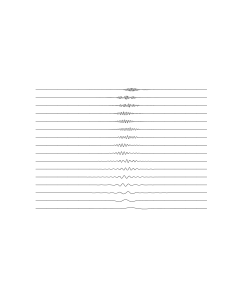
Figure 1: Wavelet packets.

4 Evaluation of Nonlinearities Scale by Scale.Non-regular approximation.

We use wavelet function $\psi(x)$, which has $k$ vanishing moments $\int x^{k}\psi(x)\mathrm{d}x=0$, or equivalently $x^{k}=\sum c_{\ell}\varphi_{\ell}(x)$ for each $k$, $0\leq k\leq K$. Let $P_{j}$ be orthogonal projector on space $V_{j}$. By tree algorithm we have for any $u\in L^{2}({\bf R})$ and $\ell\in{\bf Z}$, that the wavelet coefficients of $P_{\ell}(u)$, i.e. the set $\{<u,\psi_{j,k}>,j\leq\ell-1,k\in{\bf Z}\}$ can be compute using hierarchic algorithms from the set of scaling coefficients in $V_{\ell}$, i.e. the set $\{<u,\varphi_{\ell,k}>,k\in{\bf Z}\}$ [12]. Because for scaling function $\varphi$ we have in general only $\int\varphi(x)\mathrm{d}x=1$, therefore we have for any function $u\in L^{2}({\bf R})$:

$$\lim_{j\to\infty,k2^{-j}\to x}\mid 2^{j/2}<u,\varphi_{j,k}>-u(x)\mid=0$$ (13)

If the integer $n(\varphi)$ is the largest one such that

$$\int x^{\alpha}\varphi(x)\mathrm{d}x=0\qquad\mbox{for}\qquad 1\leq\alpha\leq n$$ (14)

then if $u\in C^{(n+1)}$ with $u^{(n+1)}$ bounded we have for $j\to\infty$ uniformly in k:

$$\mid 2^{j/2}<u,\varphi_{j,k}>-u(k2^{-j})\mid=O(2^{-j(n+1)}).$$ (15)

Such scaling functions with zero moments are very useful for us from the point of view of time-frequency localization, because we have for Fourier component $\hat{\Phi}(\omega)$ of them, that exists some $C(\varphi)\in{\bf R}$, such that for $\omega\to 0$ $\quad\hat{\Phi}(\omega)=1+C(\varphi)$ $\mid\omega\mid^{2r+2}$ (remember, that we consider r-regular multiresolution analysis). Using such type of scaling functions lead to superconvergence properties for general Galerkin approximation [12]. Now we need some estimates in each scale for non-linear terms of type $u\mapsto f(u)=f\circ u$, where f is $C^{\infty}$ (in previous and future parts we consider only truncated Taylor series action). Let us consider non regular space of approximation $\widetilde{V}$ of the form

$$\widetilde{V}=V_{q}\oplus\sum_{q\leq j\leq p-1}\widetilde{W_{j}},$$ (16)

with $\widetilde{W_{j}}\subset W_{j}$. We need efficient and precise estimate of $f\circ u$ on $\widetilde{V}$. Let us set for $q\in{\bf Z}$ and $u\in L^{2}({\bf R})$

$$\prod f_{q}(u)=2^{-q/2}\sum_{k\in{\bf Z}}f(2^{q/2}<u,\varphi_{q,k}>)\cdot\varphi_{q,k}$$ (17)

We have the following important for us estimation (uniformly in q) for $u,f(u)\in H^{(n+1)}$ [12]:

$$\|P_{q}\left(f(u)\right)-\prod f_{q}(u)\|_{L^{2}}=O\left(2^{-(n+1)q}\right)$$ (18)

For non regular spaces (16) we set

$$\prod f_{\widetilde{V}}(u)=\prod f_{q}(u)+\sum_{\ell=q,p-1}P_{\widetilde{W_{j}}}\prod f_{\ell+1}(u)$$ (19)

Then we have the following estimate:

$$\|P_{\widetilde{V}}\left(f(u)\right)-\prod f_{\widetilde{V}}(u)\|_{L^{2}}=O(2^{-(n+1)q})$$ (20)

uniformly in q and $\widetilde{V}$ (16). This estimate depends on q, not p, i.e. on the scale of the coarse grid, not on the finest grid used in definition of $\widetilde{V}$. We have for total error

$$\|f(u)-\prod f_{\widetilde{V}}(u)\|=\|f(u)-P_{\widetilde{V}}(f(u))\|_{L^{2}}$$

$$+\|P_{\widetilde{V}}(f(u)-\prod f_{\widetilde{V}}(u))\|_{L^{2}}$$ (21)

and since the projection error in $\widetilde{V}$: $\|f(u)-P_{\bar{V}}\left(f(u)\right)\|_{L^{2}}$ is much smaller than the projection error in $V_{q}$ we have the improvement (20) of (18). In concrete calculations and estimates it is very useful to consider approximations in the particular case of c-structured space:

$$\widetilde{V}= V_{q}+\sum^{p-1}_{j=q}span\{\psi_{j,k},$$

$$k\in[2^{(j-1)}-c,2^{(j-1)}+c]\quad\mbox{\rm mod}\quad 2^{j}\}$$

We are very grateful to M. Cornacchia (SLAC), W. Herrmannsfeldt (SLAC), Mrs. J. Kono (LBL) and M. Laraneta (UCLA) for their permanent encouragement.

References

- [1] Fedorova, A.N., Zeitlin, M.G. ’Wavelets in Optimization and Approximations’, Math. and Comp. in Simulation, 46, 527-534 (1998).
- [2] Fedorova, A.N., Zeitlin, M.G., ’Wavelet Approach to Polynomial Mechanical Problems’, New Applications of Nonlinear and Chaotic Dynamics in Mechanics, Kluwer, 101-108, 1998.
- [3] Fedorova, A.N., Zeitlin, M.G., ’Wavelet Approach to Mechanical Problems. Symplectic Group, Symplectic Topology and Symplectic Scales’, New Applications of Nonlinear and Chaotic Dynamics in Mechanics, Kluwer, 31-40, 1998.
- [4] Fedorova, A.N., Zeitlin, M.G ’Nonlinear Dynamics of Accelerator via Wavelet Approach’, AIP Conf. Proc., vol. 405, 87-102, 1997, Los Alamos preprint, physics/9710035.
- [5] Fedorova, A.N., Zeitlin, M.G, Parsa, Z., ’Wavelet Approach to Accelerator Problems’, parts 1-3, Proc. PAC97, vol. 2, 1502-1504, 1505-1507, 1508-1510, IEEE, 1998.
- [6] Fedorova, A.N., Zeitlin, M.G, Parsa, Z., ’Nonlinear Effects in Accelerator Physics: from Scale to Scale via Wavelets’, ’Wavelet Approach to Hamiltonian, Chaotic and Quantum Calculations in Accelerator Physics’, Proc. EPAC’98, 930-932, 933-935, Institute of Physics, 1998.
-
[7]
Fedorova, A.N., Zeitlin, M.G., Parsa, Z.,
’Variational Approach in Wavelet Framework to Polynomial
Approximations of Nonlinear Accelerator Problems’,
AIP Conf. Proc., vol. 468, 48-68, 1999.
Los Alamos preprint, physics/9902062. -
[8]
Fedorova, A.N., Zeitlin, M.G., Parsa, Z.,
’Symmetry, Hamiltonian Problems and Wavelets in
Accelerator Physics’,
AIP Conf.Proc., vol. 468, 69-93, 1999.
Los Alamos preprint, physics/9902063. - [9] Balandin, V., NSF-ITP-96-155i.
- [10] Cohen, A., Daubechies, I., Feauveau, J.C., Comm. Pure. Appl. Math., XLV, 485-560, (1992).
- [11] Hofer, E., Zehnder, E., Symplectic Topology: Birkhauser, 1994.
- [12] Liandrat, J., Tchamitchian, Ph., Advances in Comput. Math., (1996).