NONLINEAR ACCELERATOR PROBLEMS VIA WAVELETS:
3. EFFECTS OF INSERTION DEVICES ON BEAM DYNAMICS

Abstract

In this series of eight papers we present the applications of methods from wavelet analysis to polynomial approximations for a number of accelerator physics problems. In this part, assuming a sinusoidal field variation, we consider the analytical treatment of the effects of insertion devices on beam dynamics. We investigate via wavelet approach a dynamical model which has polynomial nonlinearities and variable coefficients. We construct the corresponding wavelet representation. As examples we consider wigglers and undulator magnets. We consider the further modification of our variational approach which may be applied in each scale.

1 INTRODUCTION

This is the third part of our eight presentations in which we consider applications of methods from wavelet analysis to nonlinear accelerator physics problems. This is a continuation of our results from [1]-[8], which is based on our approach to investigation of nonlinear problems – general, with additional structures (Hamiltonian, symplectic or quasicomplex), chaotic, quasiclassical, quantum, which are considered in the framework of local (nonlinear) Fourier analysis, or wavelet analysis. Wavelet analysis is a relatively novel set of mathematical methods, which gives us a possibility to work with well-localized bases in functional spaces and with the general type of operators (differential, integral, pseudodifferential) in such bases. In this part we consider effects of insertion devices (section 2) on beam dynamics. In section 3 we consider generalization of our variational approach for the case of variable coefficients. In section 4 we consider more powerful variational approach which is based on ideas of para-products and approximation for multiresolution approach, which gives us possibility for computations in each scale separately.

2 Effects of Insertion Devices on Beam Dynamics

Assuming a sinusoidal field variation, we may consider according to [9] the analytical treatment of the effects of insertion devices on beam dynamics. One of the major detrimental aspects of the installation of insertion devices is the resulting reduction of dynamic aperture. Introduction of non-linearities leads to enhancement of the amplitude-dependent tune shifts and distortion of phase space. The nonlinear fields will produce significant effects at large betatron amplitudes. The components of the insertion device magnetic field used for the derivation of equations of motion are as follows:

$$B_{x} = \frac{k_{x}}{k_{y}}\cdot B_{0}\sinh(k_{x}x)\sinh(k_{y}y)\cos(kz)$$

$$B_{y} = B_{0}\cosh(k_{x}x)\cosh(k_{y}y)\cos(kz)$$ (1)

$$B_{z} = -\frac{k}{k_{y}}B_{0}\cosh(k_{x}x)\sinh(k_{y}y)\sin(kz),$$

with $k_{x}^{2}+k_{y}^{2}=k^{2}=(2\pi/\lambda)^{2}$, where $\lambda$ is the period length of the insertion device, $B_{0}$ is its magnetic field, $\rho$ is the radius of the curvature in the field $B_{0}$. After a canonical transformation to change to betatron variables, the Hamiltonian is averaged over the period of the insertion device and hyperbolic functions are expanded to the fourth order in $x$ and $y$ (or arbitrary order). Then we have the following Hamiltonian:

$$H = \frac{1}{2}[p_{x}^{2}+p_{y}^{2}]+\frac{1}{4k^{2}\rho^{2}}[k_{x}^{2}x^{2}+k_{y}^{2}y^{2}]$$

$$+ \frac{1}{12k^{2}\rho^{2}}[k_{x}^{4}x^{4}+k_{y}^{4}y^{4}+3k_{x}^{2}k^{2}x^{2}y^{2}]$$

$$- \frac{\sin(ks)}{2k\rho}[p_{x}(k_{x}^{2}x^{2}+k_{y}^{2}y^{2})-2k_{x}p_{y}xy]$$

We have in this case also nonlinear (polynomial with degree 3) dynamical system with variable (periodic) coefficients. As related cases we may consider wiggler and undulator magnets. We have in horizontal $x-s$ plane the following equations

$$\ddot{x} = -\dot{s}\frac{e}{m\gamma}{B_{z}(s)}$$ (3)

$$\ddot{s} = \dot{x}\frac{e}{m\gamma}B_{z}(s),$$

where magnetic field has periodic dependence on $s$ and hyperbolic on $z$.

3 Variable Coefficients

In the case when we have situation when our problem is described by a system of nonlinear (polynomial)differential equations, we need to consider extension of our previous approach which can take into account any type of variable coefficients (periodic, regular or singular). We can produce such approach if we add in our construction additional refinement equation, which encoded all information about variable coefficients [10]. According to our variational approach we need to compute integrals of the form

$$\int_{D}b_{ij}(t)(\varphi_{1})^{d_{1}}(2^{m}t-k_{1})(\varphi_{2})^{d_{2}}(2^{m}t-k_{2})\mathrm{d}x,$$ (4)

where now $b_{ij}(t)$ are arbitrary functions of time, where trial functions $\varphi_{1},\varphi_{2}$ satisfy a refinement equations:

$$\varphi_{i}(t)=\sum_{k\in{\bf Z}}a_{ik}\varphi_{i}(2t-k)$$ (5)

If we consider all computations in the class of compactly supported wavelets then only a finite number of coefficients do not vanish. To approximate the non-constant coefficients, we need choose a different refinable function $\varphi_{3}$ along with some local approximation scheme

$$(B_{\ell}f)(x):=\sum_{\alpha\in{\bf Z}}F_{\ell,k}(f)\varphi_{3}(2^{\ell}t-k),$$ (6)

where $F_{\ell,k}$ are suitable functionals supported in a small neighborhood of $2^{-\ell}k$ and then replace $b_{ij}$ in (4) by $B_{\ell}b_{ij}(t)$. In particular case one can take a characteristic function and can thus approximate non-smooth coefficients locally. To guarantee sufficient accuracy of the resulting approximation to (4) it is important to have the flexibility of choosing $\varphi_{3}$ different from $\varphi_{1},\varphi_{2}$. In the case when D is some domain, we can write

$$b_{ij}(t)\mid_{D}=\sum_{0\leq k\leq 2^{\ell}}b_{ij}(t)\chi_{D}(2^{\ell}t-k),$$ (7)

where $\chi_{D}$ is characteristic function of D. So, if we take $\varphi_{4}=\chi_{D}$, which is again a refinable function, then the problem of computation of (4) is reduced to the problem of calculation of integral

$$H(k_{1},k_{2},k_{3},k_{4})=H(k)=$$

$$\int_{{\bf R}^{s}}\varphi_{4}(2^{j}t-k_{1})\varphi_{3}(2^{\ell}t-k_{2})\times$$ (8)

$$\varphi_{1}^{d_{1}}(2^{r}t-k_{3})\varphi_{2}^{d_{2}}(2^{s}t-k_{4})\mathrm{d}x$$

The key point is that these integrals also satisfy some sort of refinement equation:

$$2^{-|\mu|}H(k)=\sum_{\ell\in{\bf Z}}b_{2k-\ell}H(\ell),\qquad\mu=d_{1}+d_{2}.$$ (9)

This equation can be interpreted as the problem of computing an eigenvector. Thus, we reduced the problem of extension of our method to the case of variable coefficients to the same standard algebraical problem as in the preceding sections.

So, the general scheme is the same one and we have only one more additional linear algebraic problem by which we in the same way can parameterize the solutions of corresponding problem. As example we demonstrate on Fig. 1 a simple model of (local) intersection and the corresponding multiresolution representation (MRA).

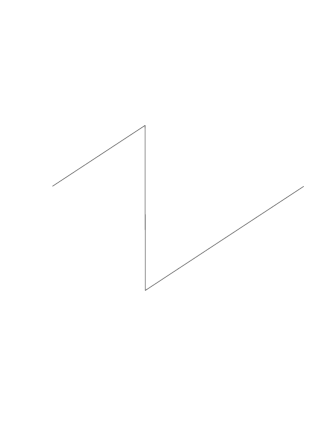
Figure 1: Simple insertion.

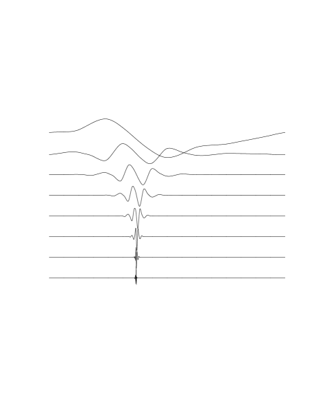
Figure 2: MRA representations.

4 Evaluation of Nonlinearities Scale by Scale

We consider scheme of modification of our variational approach in the case when we consider different scales separately. For this reason we need to compute errors of approximations. The main problems come of course from nonlinear terms. We follow the approach from [11].

Let $P_{j}$ be projection operators on the subspaces $V_{j},j\in{\bf Z}$:

$$P_{j} : L^{2}({\bf R})\to V_{j}$$ (10)

$$(P_{j}f)(x) = \sum_{k}<f,\varphi_{j,k}>\varphi_{j,k}(x)$$

and $Q_{j}$ are projection operators on the subspaces $W_{j}$:

$$Q_{j}=P_{j-1}-P_{j}$$ (11)

So, for $u\in L^{2}({\bf R})$ we have $u_{j}=P_{j}u\quad$ and $u_{j}\in V_{j}$, where $\{V_{j}\},j\in{\bf Z}$ is a multiresolution analysis of $L^{2}({\bf R})$. It is obviously that we can represent $u_{0}^{2}$ in the following form:

$$u_{0}^{2}=2\sum^{n}_{j=1}(P_{j}u)(Q_{j}u)+\sum^{n}_{j=1}(Q_{j}u)(Q_{j}u)+u_{n}^{2}$$ (12)

In this formula there is no interaction between different scales. We may consider each term of (12) as a bilinear mappings:

$$\displaystyle M_{VW}^{j}:V_{j}\times W_{j}\to L^{2}({\bf R})=V_{j}{\oplus_{j^{\prime}\geq j}W_{j^{\prime}}}$$ (13)

$$M_{WW}^{j}:W_{j}\times W_{j}\to L^{2}({\bf R})=V_{j}\oplus_{j^{\prime}\geq j}W_{j^{\prime}}$$ (14)

For numerical purposes we need formula (12) with a finite number of scales, but when we consider limits $j\to\infty$ we have

$$u^{2}=\sum_{j\in{\bf Z}}(2P_{j}u+Q_{j}u)(Q_{j}u),$$ (15)

which is para-product of Bony, Coifman and Meyer.

Now we need to expand (12) into the wavelet bases. To expand each term in (12) into wavelet basis, we need to consider the integrals of the products of the basis functions, e.g.

$$M^{j,j^{\prime}}_{WWW}(k,k^{\prime},\ell)=\int^{\infty}_{-\infty}\psi^{j}_{k}(x)\psi^{j}_{k^{\prime}}(x)\psi^{j^{\prime}}_{\ell}(x)\mathrm{d}x,$$ (16)

where $j^{\prime}>j$ and

$$\psi^{j}_{k}(x)=2^{-j/2}\psi(2^{-j}x-k)$$ (17)

are the basis functions. If we consider compactly supported wavelets then

$$M_{WWW}^{j,j^{\prime}}(k,k^{\prime},\ell)\equiv 0\quad\mbox{for}\quad|k-k^{\prime}|>k_{0},$$ (18)

where $k_{0}$ depends on the overlap of the supports of the basis functions and

$$|M_{WWW}^{r}(k-k^{\prime},2^{r}k-\ell)|\leq C\cdot 2^{-r\lambda M}$$ (19)

Let us define $j_{0}$ as the distance between scales such that for a given $\varepsilon$ all the coefficients in (19) with labels $r=j-j^{\prime}$, $r>j_{0}$ have absolute values less than $\varepsilon$. For the purposes of computing with accuracy $\varepsilon$ we replace the mappings in (13), (14) by

$$M_{VW}^{j}:V_{j}\times W_{j}\to V_{j}\oplus_{j\leq j^{\prime}\leq j_{0}}W_{j^{\prime}}$$ (20)

$$M_{WW}^{j}:W_{j}\times W_{j}\to V_{j}\oplus_{J\leq j^{\prime}\leq j_{0}}W_{j^{\prime}}$$

Since

$$V_{j}\oplus_{j\leq j^{\prime}\leq j_{0}}W_{j^{\prime}}=V_{j_{0}-1}$$ (21)

and

$$V_{j}\subset V_{j_{0}-1},\qquad W_{j}\subset V_{j_{0}-1}$$ (22)

we may consider bilinear mappings (20), (4) on $V_{j_{0}-1}\times V_{j_{0}-1}$. For the evaluation of (20), (4) as mappings $V_{j_{0}-1}\times V_{j_{0}-1}\to V_{j_{0}-1}$ we need significantly fewer coefficients than for mappings (20), (4). It is enough to consider only coefficients

$$M(k,k^{\prime},\ell)=2^{-j/2}\int^{\infty}_{\infty}\varphi(x-k)\varphi(x-k^{\prime})\varphi(x-\ell)\mathrm{d}x,$$ (23)

where $\varphi(x)$ is scale function. Also we have

$$M(k,k^{\prime},\ell)=2^{-j/2}M_{0}(k-\ell,k^{\prime}-\ell),$$ (24)

where

$$M_{0}(p,q)=\int\varphi(x-p)\varphi(x-q)\varphi(x)\mathrm{d}x$$ (25)

Now as in section (3) we may derive and solve a system of linear equations to find $M_{0}(p,q)$ and obtain explicit representation for solution.

We are very grateful to M. Cornacchia (SLAC), W. Herrmannsfeldt (SLAC), Mrs. M. Laraneta (UCLA), J. Ko-
no (LBL) for their permanent encouragement.

References

- [1] Fedorova, A.N., Zeitlin, M.G. ’Wavelets in Optimization and Approximations’, Math. and Comp. in Simulation, 46, 527-534 (1998).
- [2] Fedorova, A.N., Zeitlin, M.G., ’Wavelet Approach to Polynomial Mechanical Problems’, New Applications of Nonlinear and Chaotic Dynamics in Mechanics, Kluwer, 101-108, 1998.
- [3] Fedorova, A.N., Zeitlin, M.G., ’Wavelet Approach to Mechanical Problems. Symplectic Group, Symplectic Topology and Symplectic Scales’, New Applications of Nonlinear and Chaotic Dynamics in Mechanics, Kluwer, 31-40, 1998.
- [4] Fedorova, A.N., Zeitlin, M.G ’Nonlinear Dynamics of Accelerator via Wavelet Approach’, AIP Conf. Proc., vol. 405, 87-102, 1997, Los Alamos preprint, physics/9710035.
- [5] Fedorova, A.N., Zeitlin, M.G, Parsa, Z., ’Wavelet Approach to Accelerator Problems’, parts 1-3, Proc. PAC97, vol. 2, 1502-1504, 1505-1507, 1508-1510, IEEE, 1998.
- [6] Fedorova, A.N., Zeitlin, M.G, Parsa, Z., ’Nonlinear Effects in Accelerator Physics: from Scale to Scale via Wavelets’, ’Wavelet Approach to Hamiltonian, Chaotic and Quantum Calculations in Accelerator Physics’, Proc. EPAC’98, 930-932, 933-935, Institute of Physics, 1998.
-
[7]
Fedorova, A.N., Zeitlin, M.G., Parsa, Z.,
’Variational Approach in Wavelet Framework to Polynomial
Approximations of Nonlinear Accelerator Problems’,
AIP Conf. Proc., vol. 468, 48-68, 1999.
Los Alamos preprint, physics/9902062. -
[8]
Fedorova, A.N., Zeitlin, M.G., Parsa, Z.,
’Symmetry, Hamiltonian Problems and Wavelets in
Accelerator Physics’,
AIP Conf.Proc., vol. 468, 69-93, 1999.
Los Alamos preprint, physics/9902063. - [9] Ropert, A., CERN 98-04.
- [10] Dahmen, W., Micchelli, C., SIAM J. Numer. Anal., 30, no. 2, 507-537 (1993).
- [11] Beylkin, G., Colorado preprint, 1992.