The two–particle problem in a many–particle system:
I. Dynamically screened ladder approximation

Abstract

The two-particle problem within a nonequilibrium many-particle system is investigated in the framework of real-time Green’s functions. Starting from the dynamically screened ladder approximation of the nonequlibrium Bethe-Salpeter equation, a nonequilibrium Dyson equation is given for two-time two-particle Green’s functions. Thereby the well-known Kadanoff-Baym equations are generalized to the case of two-particle functions. The two-time structure of the equations is achieved in an exact way avoiding the so-called Shindo approximation. For the case of thermodynamic equilibrium, the differences to former results obtained for the effective two-particle hamiltonian are discussed.

I Introduction

This paper is devoted to the kinetic theory of many-particle systems which are able to form bound states. To be specific, we will consider the case of two-particle bound states, i.e. the bound states are to be thought of, e.g., as hydrogen-like atoms or ions. Our focus will be the derivation of a kinetic equation for the distribution function of the (possibly excited) bound states. Starting with papers of, for instance, Waldmann [1], Snider and Lowry [2, 3], McLennan and Lagan [4, 5, 6], Klimontovich and Kremp [7], the derivation of kinetic equations has appealed great interest over many years. Usually (see, e.g. the review article of Klimontovich et al. [8]) the two-particle density matrix is split up in different parts with respect to some projection operator which projects onto the space of the bound states. Often the states are taken to be those of the isolated atom. The diagonal matrix elements are considered to be the distribution function for the respective bound state. However, in a dense system, it is not clear if the diagonalization of the density matrix with respect to the unperturbed two-particle states is a good approximation.

It is well known that many-particle effects like dynamical screening, self-energies or phase space occupation may have an influence on the two-particle properties. A unique description of these effects within the investigation of nonequilibrium behaviour can be given in the framework of the real-time Green’s functions technique. For the single-particle functions, this can be done with the Kadanoff-Baym equations for the correlation functions $g_{a}^{\gtrless}$. In this paper we aim on the derivation of similar equations on the two-particle level.

Some remarks on the bound state problem in equilibrium seem to be useful first. The investigation of bound states in dense systems, which are in the state of thermodynamic equilibrium, has been the topic of a lot of papers, see the references cited in the monographs [9] and [10]. In the framework of the Green’s functions method, a proper starting point is the so-called Bethe-Salpeter equation for the two-particle causal Green’s function [11, 12, 13]

$$g_{ab}(12,1^{\prime}2^{\prime}) = g_{a}(1,1^{\prime})g_{b}(2,2^{\prime})$$ (2)

$$+i\int d{\bar{1}}d{\bar{2}}d{\bar{\bar{1}}}d{\bar{\bar{2}}}\,g_{a}(1,{\bar{1}})g_{b}(2,{\bar{2}})\,K_{ab}({\bar{1}}{\bar{2}},{\bar{\bar{1}}}{\bar{\bar{2}}})\,g_{ab}({\bar{\bar{1}}}{\bar{\bar{2}}},1^{\prime}2^{\prime})\,.$$

The kernel of this integral equation $K_{ab}$ is a four point function. In a diagrammatic language $K_{ab}$ comprises all irreducible diagrams in the particle-particle channel. The effective interaction $K_{ab}$ has a dynamical character. This makes the structure complicate: although one is interested only in the two-particle Green’s function in the particle-particle channel with $t_{1}=t_{2}$ and $t_{1}^{\prime}=t_{2}^{\prime}$, by the dynamical kernel $K$ the knowledge of a Green’s function with three times is enforced in the integral term. In Fourier space (or within the Matsubara technique), this is adequate to the problem that, for the determination of the two-particle Green’s function dependent on one frequency, a more general function dependent on two frequencies has to be known. A way out of this dilemma has been tried by applying the Shindo approximation [14] in which the causal quantity with two frequencies is constructed from that with one frequency. Then one gets a closed equation for the causal Green’s function. There are few estimations on the range of validity of this approximation. It is an exact relation for a static interaction $K$. It has been argued that the Shindo approximation reflects a first order approximation with respect to the retardation of the effective interaction [15, 10, 16].

In order to evaluate the Bethe-Salpeter equation, one has, of course, to use some approximation for the effective interaction $K_{ab}$. In the simplest one, which has a dynamical character, $K_{ab}$ is just the dynamically screened potential $V^{S}_{ab}$. We will come back to this point later.

With help of this Bethe-Salpeter equation, some important questions concerning the properties of two-particle states in a plasma could be discussed. An effective Schrödinger equation was derived which has some important corrections in comparison with that for an isolated atom: (i) phase space occupation factors, (ii) exchange self-energies (Hartree-Fock), (iii) a dynamically screened effective potential and (iv) dynamical single-particle self-energy corrections. It has been shown that for localized states there is to a large extent a compensation between the effects (i) and (iii) on one side and (ii) and (iv) on the other. It follows that the binding energies of (at least the low lying) bound states are not changed considerably in comparison with the isolated atom. In contrast there is a large shift of the continuum edge by the self-energy corrections. This results in a lowering of ionization energies with increasing plasma density and leads, at the end, to the well-known Mott effect. An effective wave equation was solved numerically in [17, 18], for a discussion of the result see Kraeft [19].

However, the results obtained for the effective Hamiltonian have also some serious shortcomings. There occurs a division by Pauli-blocking factors $1-f_{a}-f_{b}$ what causes spurious pole structures for highly degenerate systems. Further, the effective Hamiltonian has static contributions which lack a clear physical interpretation (see e.g. [20]). These static parts vanish for a nondegenerate system.

An other approach has been given by Schuck and co-workers [21, 22]. They postulate that Dyson equations exist for two-time causal and retarded Green’s functions, respectively. Expressions for the self-energy operator (also called mass operator or effective Hamiltonian) are derived by comparison with the respective equations of motion. It remains also unclear in this approach what approximation (if any) is connected with the assumption that such two-time Dyson equations for the investigated functions and the inverse of those functions, respectively, do exist. Also in this approach, there occours the problem of the division by Pauli-blocking factors.

Looking at the complicate structure of the Bethe-Salpeter equation, there arises the question if a general formulation in terms of a two-time Dyson equation is possible. The approach using the Shindo approximation is per se an approximative one. Schuck et al. do not consider the Bethe-Salpeter equation at all but postulate just this two-time structure. There are some strong arguments in favour of the possibility that exact equations exist for two-time Green’s functions which contain solely two-time quantities (the inner structure of a self-energy operator could be complicate, however). In a chemical picture, for instance, in which bound states are interpreted as a new species, one would expect equations for correlation functions $g^{\gtrless}_{ab}(t,t^{\prime})$ similar to the Kadanoff-Baym equations in the single-particle case with some two-particle self-energy functions. The spectral information, e.g. binding energies, damping etc., should follow from the retarded two-particle Green’s function $g^{R}_{ab}(t,t^{\prime})$. The correlation function $g^{<}_{ab}(t,t^{\prime})$ is for $t=t^{\prime}$ just the two-particle density matrix.

In nonequilibrium one can derive an equation of the same structure like in Eq. (2), however, the time integrations have to be performed then on the Keldysh contour. The functions involved in the integral term consist of many correlation functions because they are dependent on three times at least. Schäfer et al. [23] considered the dynamically screened ladder approximation for the polarizability in a semiconductor within the Keldysh formalism. They gave a formulation for functions depending on three times or – after Fourier transformation – on two frequencies. At the end, however, they used the Shindo approximation for these two-frequency quantities in order to get kinetic equations for single-frequency functions.

There were attempts to generalize the Shindo approximation to functions in the time domain [24]. It was also tried, [25], to generalize the approach of Schuck et al. within the nonequilibrium real-time Green’s functions method postulating a Dyson equation for the retarded function $g_{ab}^{R}(t,t^{\prime})=\Theta(t-t^{\prime})(g_{ab}^{>}-g_{ab}^{<})$. In both approaches similar results were achieved. The equilibrium results could be reproduced. Thus the same shortcomings arise for degenerate systems.

We will present here a new approach [26] to this problem within the real-time Green’s functions method. Thus we are able to describe nonequlibrium systems. Results for thermodynamic equlibium will appear as special case of the more general equations. In this first part the nonequilibrium Bethe-Salpeter equation is considered in a concrete approximation, the so-called dynamically screened ladder equation. This is the simplest approximation in which the effective interaction is of dynamical nature. This will enable us to identify the underlying algebraic structures and to keep the equations as simple as possible. The general scheme will be investigated in a subsequent paper [27].

The structure of this paper is as follows. In Sec. II the scheme of the real-time Green’s function method for single-particle Green’s functions is summarized. The difficulties of the Bethe-Salpeter equation are discussed in Sec. III.

The dynamically screened ladder approximation is considered in Sec. IV. The Bethe-Salpeter equation is written down in this approximation for two-time functions on the Keldysh double time contour. The first terms of the pertubation expansion with respect to the dynamically screened potential are evaluated. The two-time structure will be achieved by applying the semi-group property of the ideal propagators. After that, the algebraic structures turn out to be similar to those of the non-equilibrium Dyson-Keldysh equation in the single-particle case and the two-particle self-energy functions can be identified by comparison. The thermodynamic equilibrium case is considered in Sec. V. The structure of the two-particle self-energy which can be understood as an effective Hamiltonian is discussed. The results are compared with the former ones [12, 15, 10, 20]. It will turn out that only in the nondegenerate case and in the static limit, one is led to the same results.

II Single-particle quantities

Let us summarize shortly the scheme of real-time Green’s function technique in the single-particle case. The equations are given on a double-time contour, on the so-called Keldysh contour [28, 29]. Objects of the algebra are matrices of causal and anticausal Green’s functions, $g_{a}$ and $\overline{g}_{a}$, and the correlation functions $g_{a}^{\gtrless}$ defined below

$$g_{a}({\bf r}_{1}t,{\bf r}_{1}^{\prime}t^{\prime}) = \Theta(t-t^{\prime})g_{a}^{>}({\bf r}_{1}t,{\bf r}_{1}^{\prime}t^{\prime})+\Theta(t^{\prime}-t)g_{a}^{<}({\bf r}_{1}t,{\bf r}_{1}^{\prime}t^{\prime})$$ (3)

$$= \Theta(t-t^{\prime})\frac{1}{i}\langle\Psi_{a}({\bf r}_{1},t)\Psi_{a}^{\dagger}({\bf r}_{1}^{\prime},t^{\prime})\rangle+\Theta(t^{\prime}-t)(\pm)\frac{1}{i}\langle\Psi_{a}^{\dagger}({\bf r}_{1}^{\prime},t^{\prime})\Psi_{a}({\bf r}_{1},t)\rangle\,\,,$$ (4)

$$\overline{g}_{a}({\bf r}_{1}t,{\bf r}_{1}^{\prime}t^{\prime}) = \Theta(t-t^{\prime})g_{a}^{<}({\bf r}_{1}t,{\bf r}_{1}^{\prime}t^{\prime})+\Theta(t^{\prime}-t)g_{a}^{>}({\bf r}_{1}t,{\bf r}_{1}^{\prime}t^{\prime})\,.$$ (5)

Here $a$ is the species index, $\Psi_{a}^{\dagger}$ and $\Psi_{a}$ are creation and annihilation operators of second quantization with the commutation relations

$$[\Psi_{a}({\bf r},t),\Psi_{b}^{\dagger}({\bf r}^{\prime},t)]_{\mp} = \delta_{ab}\delta({\bf r}-{\bf r}^{\prime})$$ (6)

$$[\Psi_{a}({\bf r},t),\Psi_{b}({\bf r}^{\prime},t)]_{\mp} = 0$$ (7)

$$[\Psi^{\dagger}_{a}({\bf r},t),\Psi^{\dagger}_{b}({\bf r}^{\prime},t)]_{\mp} = 0\,.$$ (8)

The upper sign (meaning the commutator) holds for Bosons and the lower one (anticommutator) for Fermions. Spin is not written explicitely here.

One can see that these elements are not all independent. It turns out that the equations get a more convenient structure if one introduces two other quantities, $g_{a}^{R}$ and $g_{a}^{A}$, defined by

$$g_{a}^{R} = \Theta(t-t^{\prime})\frac{1}{i}\langle\Psi_{a}(r_{1},t)\Psi_{a}^{\dagger}(r_{1}^{\prime},t^{\prime})\mp\Psi_{a}^{\dagger}(r_{1}^{\prime},t^{\prime})\Psi_{a}(r_{1},t)\rangle$$ (9)

$$= \Theta(t-t^{\prime})\Big{[}g_{a}^{>}(t,t^{\prime})-g_{a}^{<}(t,t^{\prime})\Big{]}\,,$$ (10)

$$g_{a}^{A} = -\Theta(t^{\prime}-t)\frac{1}{i}\langle\Psi_{a}(r_{1},t)\Psi_{a}^{\dagger}(r_{1}^{\prime},t^{\prime})\mp\Psi_{a}^{\dagger}(r_{1}^{\prime},t^{\prime})\Psi_{a}(r_{1},t)\rangle$$ (11)

$$= \Theta(t^{\prime}-t)\Big{[}g_{a}^{<}(t,t^{\prime})-g_{a}^{>}(t,t^{\prime})\Big{]}\,.$$ (12)

It follows that

$$g_{a}^{R} = g_{a}-g_{a}^{<}=g_{a}^{>}-\overline{g}_{a}\,,$$ (13)

$$g_{a}^{A} = g_{a}-g_{a}^{>}=g_{a}^{<}-\overline{g}_{a}\,.$$ (14)

The nonequlilibrium Dyson equation on the Keldysh contour reads

$${\underline{g}}_{a}(1,1^{\prime}) = {\underline{g}}_{a,0}(1,1^{\prime})+\int\limits_{\cal C}d{\bar{1}}d{\bar{\bar{1}}}\,{\underline{g}}_{a,0}(1,{\bar{1}})\,{\underline{\Sigma}}_{a}({\bar{1}},{\bar{\bar{1}}})\,{\underline{g}}_{a}({\bar{\bar{1}}},1^{\prime})\,,$$ (15)

with $1={\bf r}_{1},t_{1}$ etc., and ${\underline{g}}_{a,0}$ being the ideal functions and $\Sigma_{a}$ the self-energy. The time integrations are performed on the Keldysh contour, see Fig. 1. The underlined quantities are causal ones for both times on the upper branch of the contour, $g_{a}=g_{a}^{++}$, and anticausal ones for both times on the lower branch, ${\overline{g}}_{a}=g_{a}^{--}$. If the first time is on the upper branch and the second one on the lower, one gets $g_{a}^{<}=g_{a}^{+-}$. Fixing the first time on the lower and the second time on the upper branch gives $g_{a}^{>}=g_{a}^{-+}$. Working on the Keldysh contour has the advantage that well-developed schemes of functional derivatives and diagrammatic techniques known from equilibrium [30, 31] can easily be generalized to nonequilibrium situations, see, e.g., [29, 32, 33, 34].

Eq. (15) is equivalent to a set of four equations which are, however, not all independent. Therefore, it is often more convenient to work with the following form of the nonequlibrium Dyson equation for the correlation function $g_{a}^{<}$

$$g_{a}^{<}(t,t^{\prime}) = g^{<}_{a,0}(t,t^{\prime})+\int\limits_{t_{0}}^{\infty}dt_{1}\,\int\limits_{t_{0}}^{\infty}dt_{2}\,\Big{[}g^{<}_{a,0}(t,t_{1})\,\Sigma_{a}^{A}(t_{1},t_{2})\,g_{a}^{A}(t_{2},t^{\prime})$$ (17)

$$+g^{R}_{a,0}(t,t_{1})\,\Sigma_{a}^{<}(t_{1},t_{2})\,g_{a}^{A}(t_{2},t^{\prime})+g^{R}_{a,0}(t,t_{1})\,\Sigma_{a}^{R}(t_{1},t_{2})\,g_{a}^{<}(t_{2},t^{\prime})\Big{]}\,,$$

which has to be supplemented by an equation for $g_{a}^{R/A}$

$$g_{a}^{R}(t,t^{\prime}) = g^{R}_{a,\,0}(t,t^{\prime})+\int\limits_{t_{0}}^{\infty}dt_{1}\,\int\limits_{t_{0}}^{\infty}dt_{2}\,g^{R}_{a,\,0}(t,t_{1})\,\Sigma_{a}^{R}(t_{1},t_{2})\,g_{a}^{R}(t_{2},t^{\prime})\,.$$ (18)

Here only the functions’s dependence on the times was written explicitely in order to save space. Often the initial time is considered in the limit $t_{0}\longrightarrow-\infty$. The quantity $g_{a}^{A}$ is connected with $g_{a}^{R}$ by hermitean conjugation

$$g_{a}^{A}({\bf r}t,{\bf r}^{\prime}t^{\prime})=\left[g_{a}^{R}({\bf r}^{\prime}t^{\prime},{\bf r}t)\right]^{\ast}\,.$$ (19)

An other form of Eq. (17) one can find is [32]

$$g_{a}^{<}(t,t^{\prime}) = g_{a}^{R}(t,t_{0})\,g^{<}_{a}(t_{0},t_{0})\,g^{A}_{a}(t_{0},t^{\prime})+\int\limits_{t_{0}}^{\infty}dt_{1}\,\int\limits_{t_{0}}^{\infty}dt_{2}\,g^{R}_{a}(t,t_{1})\,\Sigma_{a}^{<}(t_{1},t_{2})\,g_{a}^{A}(t_{2},t^{\prime})\,.$$ (20)

The corresponding differential equations read

$$\left[i\frac{\partial}{\partial t}+\frac{\nabla^{2}}{2m_{a}}\right]\,g_{a}^{<}(t,t^{\prime}) = \int d{\bar{t}}\,\Big{[}\Sigma_{a}^{R}(t,{\bar{t}})\,g_{a}^{<}({\bar{t}},t^{\prime})+\Sigma_{a}^{<}(t,{\bar{t}})\,G_{a}^{A}({\bar{t}},t^{\prime})\Big{]}\,,$$ (21)

$$\left[i\frac{\partial}{\partial t}+\frac{\nabla^{2}}{2m_{a}}\right]\,g_{a}^{R}(t,t^{\prime}) = \delta(t-t^{\prime})+\int d{\bar{t}}\,\Sigma_{a}^{R}(t,{\bar{t}})\,g_{a}^{R}({\bar{t}},t^{\prime})\,.$$ (22)

These are the well-known generalized kinetic equations (Kadanoff-Baym equations) for the single-particle functions.

In the following chapters the one-particle self-energy will be needed in a special approximation which is called $V^{S}$-approximation. Here one has

$${\underline{\Sigma}}_{a}(1,1^{\prime}) = {\underline{\Sigma}}_{a}^{H}+i{\underline{V}}^{S\,}_{aa}(1,1^{\prime})\,{\underline{g}}_{a}(1,1^{\prime})\,,$$ (23)

with $\Sigma^{H}$ being the Hartree self-energy. As for the Green’s functions, cf. Eqs. (3,13), there is a set of functions describing the dynamically screened interaction ${\underline{V}}_{ab}^{S}$

$$V^{S}_{ab}(t,t^{\prime}) = V_{ab}\,\delta(t-t^{\prime})+\Theta(t-t^{\prime})V_{ab}^{S\,>}(t,t^{\prime})+\Theta(t^{\prime}-t)V_{ab}^{S\,<}(t,t^{\prime})\,,$$ (24)

$$\overline{V}^{S}_{ab}(t,t^{\prime}) = -V_{ab}\,\delta(t-t^{\prime})+\Theta(t-t^{\prime})V_{ab}^{S\,<}(t,t^{\prime})+\Theta(t^{\prime}-t)V_{ab}^{S\,>}(t,t^{\prime})\,,$$ (25)

$$V_{ab}^{S\,R}(t,t^{\prime}) = V_{ab}\,\delta(t-t^{\prime})+\Theta(t-t^{\prime})\Big{[}V_{ab}^{S\,>}(t,t^{\prime})-V_{ab}^{S\,<}(t,t^{\prime})\Big{]}\,,$$ (26)

$$V_{ab}^{S\,A}(t,t^{\prime}) = V_{ab}\,\delta(t-t^{\prime})+\Theta(t^{\prime}-t)\Big{[}V_{ab}^{S\,<}(t,t^{\prime})-V_{ab}^{S\,>}(t,t^{\prime})\Big{]}\,.$$ (27)

Here the correlation functions are defined by

$$V_{ab}^{S\,\gtrless}(t,t^{\prime})=\sum_{c,d}V_{ac}L^{\gtrless}_{cd}(t,t^{\prime})V_{db}\,,$$ (28)

where $L^{\gtrless}$ are the correlation functions of density fluctuations

$$iL_{ab}^{>}({\bf r}_{1}t_{1},{\bf r}_{2}t_{2}) = \langle\delta\hat{\rho}_{a}({\bf r}_{1},t_{1})\delta\hat{\rho}_{b}({\bf r}_{2},t_{2})\rangle\,,$$ (29)

$$iL_{ab}^{<}({\bf r}_{1}t_{1},{\bf r}_{2}t_{2}) = \langle\delta\hat{\rho}_{b}({\bf r}_{2},t_{2})\delta\hat{\rho}_{a}({\bf r}_{1},t_{1})\rangle\,,$$ (30)

with $\delta\hat{\rho}_{a}({\bf r},t)=\Psi_{a}^{\dagger}({\bf r},t)\Psi_{a}({\bf r},t)-\langle\Psi_{a}^{\dagger}({\bf r},t)\Psi_{a}({\bf r},t)\rangle$.
It follows that, e.g., $V_{ab}^{S\,<}(1,1^{\prime})=V_{ba}^{S\,>}(1^{\prime},1)$ and $V_{ab}^{S}(1,1^{\prime})=V_{ba}^{S}(1^{\prime},1)$, but $V_{ab}^{S\,R}(1,1^{\prime})=V_{ba}^{S\,A}(1^{\prime},1)$.

III Bethe-Salpeter equation

The two-particle Green’s function is determined by the so-called Bethe-Salpeter equation

$$g_{ab}(12,1^{\prime}2^{\prime}) = g_{a}(1,1^{\prime})g_{b}(2,2^{\prime})$$ (32)

$$+i\int d{\bar{1}}d{\bar{2}}d{\bar{\bar{1}}}d{\bar{\bar{2}}}\,g_{a}(1,{\bar{1}})g_{b}(2,{\bar{2}})\,K_{ab}({\bar{1}}{\bar{2}},{\bar{\bar{1}}}{\bar{\bar{2}}})\,g_{ab}({\bar{\bar{1}}}{\bar{\bar{2}}},1^{\prime}2^{\prime})\,,$$

in which by introduction of the effective interaction kernel $K_{ab}$ formally a closed equation is achieved for the four-point function. Here, the kernel $K_{ab}$ is the sum of all diagrams irreducible with respect to a cutting of two single-particle lines. The Bethe-Salpeter equation can be understood to hold in various contexts: for $T=0$, for the imaginary-time equilibrium Green’s functions in the Matsubara technique, or for the real-time Green’s functions on the Keldysh contour.

The properties of a pair of particles should follow from this equation in the so-called particle-particle channel. If one considers the causal two-particle Green’s function in this channel ($t_{1}=t_{2}=t;t_{1}^{\prime}=t_{2}^{\prime}=t^{\prime}$), one has

$$i^{2}g_{ab}(r_{1}r_{2}t,r_{1}^{\prime}r_{2}^{\prime}t^{\prime}) = \theta(t-t^{\prime})\Big{\langle}\Psi_{a}({\bf r}_{1},t)\Psi_{b}({\bf r}_{2},t)\Psi_{b}^{\dagger}({\bf r}_{2}^{\prime},t^{\prime})\Psi_{a}^{\dagger}({\bf r}_{1}^{\prime},t^{\prime})\Big{\rangle}$$ (33)

$$+ \theta(t^{\prime}-t)\Big{\langle}\Psi_{a}^{\dagger}({\bf r}_{1}^{\prime},t^{\prime})\Psi_{b}^{\dagger}({\bf r}_{2}^{\prime},t^{\prime})\Psi_{b}({\bf r}_{2},t)\Psi_{a}({\bf r}_{1},t)\Big{\rangle}$$ (34)

$$= \theta(t-t^{\prime})i^{2}g_{ab}^{>}+\theta(t^{\prime}-t)i^{2}g_{ab}^{<}\,.$$ (35)

On the right hand side of Eq. (32), however, there occurs a function depending on three times ${\bar{t}}_{1}$, ${\bar{t}}_{2}$, and $t^{\prime}$ what is enforced by the dynamical character of $K_{ab}$. This Green’s function consists of six different correlation functions

$$i^{2}\,g_{ab}({\bar{r}}_{1}{\bar{t}}_{1}{\bar{r}}_{2}{\bar{t}}_{2};r_{1}^{\prime}r_{2}^{\prime}t^{\prime}) = \theta({\bar{t}}_{1}-{\bar{t}}_{2})\theta({\bar{t}}_{2}-t^{\prime})\Big{\langle}\Psi_{a}({\bar{\bf r}}_{1},{\bar{t}}_{1})\Psi_{b}({\bar{\bf r}}_{2},{\bar{t}}_{2})\Psi_{b}^{\dagger}({\bf r}_{2}^{\prime},t^{\prime})\Psi_{a}^{\dagger}({\bf r}_{1}^{\prime},t^{\prime})\Big{\rangle}$$ (36)

$$\pm \theta({\bar{t}}_{2}-{\bar{t}}_{1})\theta({\bar{t}}_{1}-t^{\prime})\Big{\langle}\Psi_{b}({\bar{\bf r}}_{2},{\bar{t}}_{2})\Psi_{a}({\bar{\bf r}}_{1},{\bar{t}}_{1})\Psi_{b}^{\dagger}({\bf r}_{2}^{\prime},t^{\prime})\Psi_{a}^{\dagger}({\bf r}_{1}^{\prime},t^{\prime})\Big{\rangle}$$ (37)

$$+ \theta({\bar{t}}_{1}-t^{\prime})\theta(t^{\prime}-{\bar{t}}_{2})\Big{\langle}\Psi_{a}({\bar{\bf r}}_{1},{\bar{t}}_{1})\Psi_{b}^{\dagger}({\bf r}_{2}^{\prime},t^{\prime})\Psi_{a}^{\dagger}({\bf r}_{1}^{\prime},t^{\prime})\Psi_{b}({\bar{\bf r}}_{2},{\bar{t}}_{2})\Big{\rangle}$$ (38)

$$+ \theta({\bar{t}}_{2}-t^{\prime})\theta(t^{\prime}-{\bar{t}}_{1})\Big{\langle}\Psi_{b}({\bar{\bf r}}_{2},{\bar{t}}_{2})\Psi_{a}^{\dagger}({\bf r}_{1}^{\prime},t^{\prime})\Psi_{b}^{\dagger}({\bf r}_{2}^{\prime},t^{\prime})\Psi_{a}({\bar{\bf r}}_{1},{\bar{t}}_{1})\Big{\rangle}$$ (39)

$$\pm \theta(t^{\prime}-{\bar{t}}_{1})\theta({\bar{t}}_{1}-{\bar{t}}_{2})\Big{\langle}\Psi_{a}^{\dagger}({\bf r}_{1}^{\prime},t^{\prime})\Psi_{b}^{\dagger}({\bf r}_{2}^{\prime},t^{\prime})\Psi_{a}({\bar{\bf r}}_{1},{\bar{t}}_{1})\Psi_{b}({\bar{\bf r}}_{2},{\bar{t}}_{2})\Big{\rangle}$$ (40)

$$+ \theta(t^{\prime}-{\bar{t}}_{2})\theta({\bar{t}}_{2}-{\bar{t}}_{1})\Big{\langle}\Psi_{a}^{\dagger}({\bf r}_{1}^{\prime},t^{\prime})\Psi_{b}^{\dagger}({\bf r}_{2}^{\prime},t^{\prime})\Psi_{b}({\bar{\bf r}}_{2},{\bar{t}}_{2})\Psi_{a}({\bar{\bf r}}_{1},{\bar{t}}_{1})\Big{\rangle}\,.$$ (41)

Only a static interaction in (32) would enforce ${\bar{t}}_{1}={\bar{t}}_{2}$, and the function would turn into the two-time causal one (33).

In principle, one could of course try to solve the Bethe-Salpeter equation for a function depending on three times (equivalent to a function depending on two frequencies) and then extract from this the information one is interested in. This, however seems to be to complicated. In a number of papers it was tried therefore to work with equations which involve exclusively two-time functions. This was achieved in two ways. The first approach [12, 13] uses within the Matsubara technique the so-called Shindo approximation in which the two-frequency function is constructed from the single-frequency causal Green’s function. This is possible in an exact way for a statical interaction and therefore it was argued that for arbitrary $K_{ab}$ this would be correct in first order with respect to the retardation. In the other approach [21], a closed equation for the causal two-time or single-freqency, respectively, function is postulated. The effective hamiltonian (two-particle self-energy) is determined then by comparison with equations of motion.

In any case there are closed equations for combinations of the correlation functions $g_{ab}^{\gtrless}$ defined in (33). But this means that the information contained in the correlation functions $\langle\Psi_{a}\Psi_{b}^{\dagger}\Psi_{a}^{\dagger}\Psi_{b}\rangle$ and $\langle\Psi_{b}\Psi_{a}^{\dagger}\Psi_{b}^{\dagger}\Psi_{a}\rangle$ (third and fourth term in Eq. 36) is neglected. Therefore such a closed equation for the causal two-time Green’s function can exist only in an approximate way.

In the next section we will show that closed equations exist for other combinations of correlation functions.

IV Dynamically screened ladder approximation

In analogy to the single-particle case, one is interested to get information on the statistical properties, carried by the two-particle density matrix, as well as information on the two-particle dynamics, the spectral information. Below we will see that it is not a trivial question to say which quantity carries this information.

One of the quantities of interest is the following two-time correlation function

$$g^{<}_{ab}({\bf r}_{1}{\bf r}_{2}t,{\bf r}_{1}^{\prime}{\bf r}_{2}^{\prime}t^{\prime}\,)=\frac{1}{i^{2}}\Big{\langle}\Psi_{a}^{\dagger}({\bf r}_{1}^{\prime},t^{\prime})\Psi_{b}^{\dagger}({\bf r}_{2}^{\prime},t^{\prime})\Psi_{b}({\bf r}_{2},t)\Psi_{a}({\bf r}_{1},t)\Big{\rangle}\,.$$ (42)

In the case $t^{\prime}=t$, the quantity $i^{2}\,g_{ab}^{<}$ is just the two-particle density matrix $\rho_{ab}({\bf r}_{1}{\bf r}_{2}{\bf r}_{1}^{\prime}{\bf r}_{2}^{\prime},t\,)$.

We will use in the following the real-time Green’s function technique in the Keldysh formulation. In the present section the Bethe-Salpeter equation will be considered in a concrete approximation: for the effective interaction kernel $K_{ab}$, the dynamically screened potential $V^{S}_{ab}$ is taken. Then one has on the Keldysh contour

$${\underline{g}}_{ab}(t_{1}t_{2},t_{1}^{\prime}t_{2}^{\prime})={\underline{g}}_{a}(t_{1},t_{1}^{\prime})\,{\underline{g}}_{b}(t_{2},t_{2}^{\prime})+\int_{\cal C}d{\bar{t}}_{1}\,d{\bar{t}}_{2}\,{\underline{g}}_{a}(t_{1},{\bar{t}}_{1})\,{\underline{g}}_{b}(t_{2},{\bar{t}}_{2})\,i\underline{V}_{ab}^{S}({\bar{t}}_{1},{\bar{t}}_{2}){\underline{g}}_{ab}({\bar{t}}_{1}{\bar{t}}_{2},t_{1}^{\prime}t_{2}^{\prime})\,.$$ (43)

Iteration of this integral equation leads to ladder-type terms.

This Bethe-Salpeter equation (43) will be considered in the following in the special case $t_{1}=t_{2}=t$ and $t_{1}^{\prime}=t_{2}^{\prime}=t^{\prime}$.

A Two-particle Green’s functions depending on two times

Although the physical times $t_{1}$ and $t_{2}$ as well as $t_{1}^{\prime}$ and $t_{2}^{\prime}$ are equal, there are still 16 possibilities to fix the times $t_{1},t_{2},t_{1}^{\prime},$ and $t_{2}^{\prime}$ on the upper and lower branches of the Keldysh contour. Fixing the times $t_{1}$ and $t_{2}$ on the upper and $t_{1}^{\prime}$ and $t_{2}^{\prime}$ on the lower branch of the Keldysh contour, one gets an equation for the correlation function $g_{ab}^{++,--}=g_{ab}^{<}$ defined in Eq. (42). Below there are given three other important cases.

$$g_{ab}^{+-,-+}({\bf r}_{1}{\bf r}_{2}t,{\bf r}_{1}^{\prime}{\bf r}_{2}^{\prime}t^{\prime}\,) = \Theta(t-t^{\prime})\frac{1}{i^{2}}\Big{\langle}\Psi_{a}^{\dagger}({\bf r}_{1}^{\prime},t^{\prime})\Psi_{b}({\bf r}_{2},t)\Psi_{a}({\bf r}_{1},t)\Psi_{b}^{\dagger}({\bf r}_{2}^{\prime},t^{\prime})\Big{\rangle}$$ (45)

$$+\Theta(t^{\prime}-t)\frac{1}{i^{2}}\Big{\langle}\Psi_{b}({\bf r}_{2},t)\Psi_{a}^{\dagger}({\bf r}_{1}^{\prime},t^{\prime})\Psi_{b}^{\dagger}({\bf r}_{2}^{\prime},t^{\prime})\Psi_{a}({\bf r}_{1},t)\Big{\rangle}\,,$$

$$g_{ab}^{-+,+-}({\bf r}_{1}{\bf r}_{2}t,{\bf r}_{1}^{\prime}{\bf r}_{2}^{\prime}t^{\prime}\,) = \Theta(t-t^{\prime})\frac{1}{i^{2}}\Big{\langle}\Psi_{b}^{\dagger}({\bf r}_{2}^{\prime},t^{\prime})\Psi_{a}({\bf r}_{1},t)\Psi_{b}({\bf r}_{2},t)\Psi_{a}^{\dagger}({\bf r}_{1}^{\prime},t^{\prime})\Big{\rangle}$$ (47)

$$+\Theta(t^{\prime}-t)\frac{1}{i^{2}}\Big{\langle}\Psi_{a}({\bf r}_{1},t)\Psi_{b}^{\dagger}({\bf r}_{2}^{\prime},t^{\prime})\Psi_{a}^{\dagger}({\bf r}_{1}^{\prime},t^{\prime})\Psi_{b}({\bf r}_{2},t)\Big{\rangle}\,,$$

$$g_{ab}^{--,++}({\bf r}_{1}{\bf r}_{2}t,{\bf r}_{1}^{\prime}{\bf r}_{2}^{\prime}t^{\prime}\,) = \frac{1}{i^{2}}\Big{\langle}\Psi_{a}({\bf r}_{1},t)\Psi_{b}({\bf r}_{2},t)\Psi_{b}^{\dagger}({\bf r}_{2}^{\prime},t^{\prime})\Psi_{a}^{\dagger}({\bf r}_{1}^{\prime},t^{\prime})\Big{\rangle}\,.$$ (48)

To give an example, the time-ordering on the Keldysh contour is shown for $g_{ab}^{+-,-+}$ in Fig. 1. All other functions $g_{ab}^{\alpha\beta,\gamma\delta}$ with the greek indices equal to “$+$” or “$-$” can be expressed in terms of the six correlation functions involved in Eqs. (42) and (45-48).

We define the following retarded and advanced quantities

$$G_{ab}^{R}({\bf r}_{1}{\bf r}_{2}t,{\bf r}_{1}^{\prime}{\bf r}_{2}^{\prime}t^{\prime}\,) \equiv \Theta(t-t^{\prime})i\Big{(}g_{ab}^{++,--}-g_{ab}^{+-,-+}-g_{ab}^{-+,+-}+g_{ab}^{--,++}\Big{)}$$ (49)

$$= \Theta(t-t^{\prime})\frac{1}{i}\Big{\langle}\Big{[}\Psi_{a}^{\dagger}({\bf r}_{1}^{\prime},t^{\prime}),\Big{[}\Psi_{b}^{\dagger}({\bf r}_{2}^{\prime},t^{\prime}),\Psi_{b}({\bf r}_{2},t)\Psi_{a}({\bf r}_{1},t)\Big{]}_{-}\,\Big{]}_{\mp}\,\Big{\rangle}\,,$$ (50)

$$G_{ab}^{A}({\bf r}_{1}{\bf r}_{2}t,{\bf r}_{1}^{\prime}{\bf r}_{2}^{\prime}t^{\prime}\,) \equiv \Theta(t^{\prime}-t)(-i)\Big{(}g_{ab}^{++,--}-g_{ab}^{+-,-+}-g_{ab}^{-+,+-}+g_{ab}^{--,++}\Big{)}$$ (51)

$$= \Theta(t^{\prime}-t)\frac{1}{-i}\Big{\langle}\Big{[}\Psi_{a}({\bf r}_{1},t),\Big{[}\Psi_{b}({\bf r}_{2},t),\Psi_{b}^{\dagger}({\bf r}_{2}^{\prime},t^{\prime})\Psi_{a}^{\dagger}({\bf r}_{1}^{\prime},t^{\prime})\Big{]}_{-}\,\Big{]}_{\mp}\,\Big{\rangle}\,.$$ (52)

In order to achieve the nested commutator structures, it was used that operators with equal times can be interchanged according to (6). Interestingly enough these nested structures were found also by Rajagopal and Majumdar in their analysis of double dispersion relations for the two-frequency causal Matsubara Green’s function (Appendix II of [11]). We show in Appendix C as an example how the function $G_{ab}^{A}$ is connected in thermodynamic equilibrium with the analytic continuation of the two-frequency Matsubara Green’s function.

The functions $G_{ab}^{R/A}$ have the following properties:
(i) They are connected by hermitean conjugation

$$G_{ab}^{R}({\bf r}_{1}{\bf r}_{2}t,{\bf r}_{1}^{\prime}{\bf r}_{2}^{\prime}t^{\prime})=\Big{[}G_{ab}^{A}({\bf r}_{1}^{\prime}{\bf r}_{2}^{\prime}t^{\prime},{\bf r}_{1}{\bf r}_{2}t)\Big{]}^{\dagger}\,.$$ (53)

(ii) Both functions have the property of crossing symmetry, i.e.

$$G_{ab}^{R/A}({\bf r}_{1}{\bf r}_{2}t,{\bf r}_{1}^{\prime}{\bf r}_{2}^{\prime}t^{\prime})=G_{ba}^{R/A}({\bf r}_{2}{\bf r}_{1}t,{\bf r}_{2}^{\prime}{\bf r}_{1}^{\prime}t^{\prime})\,.$$ (54)

(iii) The inhomogeneity in the equations of motion for these functions consists of $\delta$-functions only (without Pauli-blocking terms). This is easy to see from Eqs. (49,51). Derivation of the Heaviside-function gives a $\delta$-function $\delta(t-t^{\prime})$, and the commutation relations for the field operators lead to $[\delta({\bf r}_{1}-{\bf r}_{1}^{\prime})\delta({\bf r}_{2}-{\bf r}_{2}^{\prime})\pm\delta_{ab}\delta({\bf r}_{1}-{\bf r}_{2}^{\prime})\delta({\bf r}_{2}-{\bf r}_{1}^{\prime})]$.
(iv) For vanishing interaction between the particles $a$ and $b$, the correlation functions in Eqs. (49,51) can be contracted into products of single-particle correlation functions $g^{\gtrless}$, and one gets

$$G_{ab}^{R}({\bf r}_{1}{\bf r}_{2}t,{\bf r}_{1}^{\prime}{\bf r}_{2}^{\prime}t^{\prime}\,) = i\,g_{a}^{R}({\bf r}_{1}t,{\bf r}_{1}^{\prime}t^{\prime})g_{b}^{R}({\bf r}_{2}t,{\bf r}_{2}^{\prime}t^{\prime})\pm\delta_{ab}\,i\,g_{a}^{R}({\bf r}_{1}t,{\bf r}_{2}^{\prime}t^{\prime})g_{b}^{R}({\bf r}_{2}t,{\bf r}_{1}^{\prime}t^{\prime})\,,$$ (55)

with the retarded single-particle function $g_{a}^{R}$ defined by Eq. (9).
(v) The difference of the retarded and the advanced functions defines a spectral function

$$A_{ab}({\bf r}_{1}{\bf r}_{2}t,{\bf r}_{1}^{\prime}{\bf r}_{2}^{\prime}t^{\prime}\,) = iG_{ab}^{R}({\bf r}_{1}{\bf r}_{2}t,{\bf r}_{1}^{\prime}{\bf r}_{2}^{\prime}t^{\prime}\,)-iG_{ab}^{A}({\bf r}_{1}{\bf r}_{2}t,{\bf r}_{1}^{\prime}{\bf r}_{2}^{\prime}t^{\prime}\,)$$ (56)

$$= i^{2}\Big{[}g_{ab}^{++,--}-g_{ab}^{+-,-+}-g_{ab}^{-+,+-}+g_{ab}^{--,++}\Big{]}\,,$$ (57)

which gives in the case of equal times ($t=t^{\prime}$)

$$A_{ab}({\bf r}_{1}{\bf r}_{2}t,{\bf r}_{1}^{\prime}{\bf r}_{2}^{\prime}t\,)=\delta({\bf r}_{1}-{\bf r}_{1}^{\prime})\delta({\bf r}_{2}-{\bf r}_{2}^{\prime})\pm\delta_{ab}\delta({\bf r}_{1}-{\bf r}_{2}^{\prime})\delta({\bf r}_{2}-{\bf r}_{1}^{\prime})\,.$$ (58)

B Transformation of the Bethe-Salpeter equation into a Dyson equation

In this subsection the dynamically screened ladder equation as a special approximation of the BSE is transformed into a Dyson equation in which the occuring two-particle Green’s functions and two-particle self-energy functions are dependent on two times only. For this purpose, the perturbation expansion of the Bethe-Salpeter equation (43) is considered in the diagrammatic form shown in Fig. 2. It is analyzed first for $g_{ab}^{<}$; details are presented for different orders of $V_{ab}^{S}$ in Appendix A.

We search for (and, indeed, find) the following structures [cf. the corresponding equations for the single-particle functions, Eqs. 17 and 18]

$$g^{<}_{ab} = {\cal G}^{<}_{ab}+{\cal G}^{R}_{ab}\Big{[}V_{ab}+\Sigma^{R}_{ab}\Big{]}g_{ab}^{<}+{\cal G}^{R}_{ab}\sigma^{<}_{ab}G_{ab}^{A}+{\cal G}^{<}_{ab}\Big{[}V_{ab}+\Sigma^{A}_{ab}\Big{]}G_{ab}^{A}$$ (59)

$$G^{A}_{ab} = {\cal G}^{A}_{ab}+{\cal G}^{A}_{ab}\Big{[}V_{ab}+\Sigma^{A}_{ab}\Big{]}\,G^{A}_{ab}$$ (60)

with the definitions ${\cal G}^{<}_{ab}(t,t^{\prime})=g^{<}_{a,0}(t,t^{\prime})\,g^{<}_{b,0}(t,t^{\prime})\,$, ${\cal G}^{R}_{ab}(t,t^{\prime})=ig^{R}_{a,0}(t,t^{\prime})\,g^{R}_{b,0}(t,t^{\prime})\,$, and ${\cal G}^{A}_{ab}(t,t^{\prime})=(-i)g^{A}_{a,0}(t,t^{\prime})\,g^{A}_{b,0}(t,t^{\prime})\,$. All quantities in the above equations depend on two times only. The integration of intermediate times runs in the interval $[t_{0},\infty]$ like in Eqs. (17,18).

The zeroth, first and second orders for $g_{ab}^{<}$ with respect to the two-particle self-energy are given by

$$g^{<\,(0)}_{ab} = {\cal G}^{<}_{ab}\,,$$ (61)

$$g^{<\,(1)}_{ab} = {\cal G}^{R}_{ab}\Big{[}V_{ab}+\Sigma^{R}_{ab}\Big{]}{\cal G}_{ab}^{<}+{\cal G}^{R}_{ab}\sigma^{<}_{ab}{\cal G}_{ab}^{A}+{\cal G}^{<}_{ab}\Big{[}V_{ab}+\Sigma^{A}_{ab}\Big{]}{\cal G}_{ab}^{A}\,,$$ (62)

$$g^{<\,(2)}_{ab} = {\cal G}^{R}_{ab}\Big{[}V_{ab}+\Sigma^{R}_{ab}\Big{]}{\cal G}^{R}_{ab}\Big{[}V_{ab}+\Sigma^{R}_{ab}\Big{]}{\cal G}_{ab}^{<}+{\cal G}^{R}_{ab}\Big{[}V_{ab}+\Sigma^{R}_{ab}\Big{]}{\cal G}^{R}_{ab}\sigma^{<}_{ab}{\cal G}_{ab}^{A}$$ (65)

$$+{\cal G}^{R}_{ab}\Big{[}V_{ab}+\Sigma^{R}_{ab}\Big{]}{\cal G}^{<}_{ab}\Big{[}V_{ab}+\Sigma^{A}_{ab}\Big{]}{\cal G}_{ab}^{A}+{\cal G}^{R}_{ab}\sigma^{<}_{ab}{\cal G}_{ab}^{A}\Big{[}V_{ab}+\Sigma^{A}_{ab}\Big{]}{\cal G}_{ab}^{A}$$

$$+{\cal G}^{<}_{ab}\Big{[}V_{ab}+\Sigma^{A}_{ab}\Big{]}{\cal G}_{ab}^{A}\Big{[}V_{ab}+\Sigma^{A}_{ab}\Big{]}{\cal G}_{ab}^{A}\,.$$

The self-energy functions $\sigma_{ab}^{<}$ and $\Sigma_{ab}^{R}$, respectively, are identified by comparison with the expansion terms of the ladder equation, Fig. 2, then.

All functions in the above equations (59) and (60) are understood to depend on two times. The key idea in order to achieve such a two-time structure of the equations is to use the semi-group properties of the ideal single-particle propagators $g_{a,0}^{R}$ and $g_{a,0}^{A}$ (the time-local Hartree-Fock self-energy could also be included). In particular one has for any time ${\bar{t}}$ with $t>{\bar{t}}>t^{\prime}$ the following relation

$$g_{a,0}^{R}({\bf r}_{1}t,{\bf r}_{1}^{\prime}t^{\prime})=i\int d^{3}r_{2}\,g_{a,0}^{R}({\bf r}_{1}t,{\bf r}_{2}{\bar{t}})\,g_{a,0}^{R}({\bf r}_{2}{\bar{t}},{\bf r}_{1}^{\prime}t^{\prime})\,.$$ (66)

There is no time integration in the above equation. Analogeously, for the advanced function with $t<{\bar{t}}<t^{\prime}$ one has (integration with respect to ${\bf r}_{2}$ suppressed)

$$g_{a,0}^{A}(t,t^{\prime})=(-i)\,g_{a,0}^{A}(t,{\bar{t}})\,g_{a,0}^{A}({\bar{t}},t^{\prime})\,.$$ (67)

For the ideal one-particle correlation functions $g_{a,0}^{\gtrless}$, there follows

$$g_{a,0}^{\gtrless}(t,t^{\prime}) = i\,g_{a,0}^{R}(t,{\bar{t}})\,g_{a,0}^{\gtrless}({\bar{t}},t^{\prime})\,\quad\mbox{for}\quad t>{\bar{t}}\,,$$ (68)

$$g_{a,0}^{\gtrless}(t,t^{\prime}) = (-i)\,g_{a,0}^{\gtrless}(t,{\bar{t}})\,g_{a,0}^{A}({\bar{t}},t^{\prime})\,\quad\mbox{for}\quad{\bar{t}}<t^{\prime}\,,$$ (69)

$$g_{a,0}^{\gtrless}(t,t^{\prime}) = (-i^{2})\,g_{a,0}^{R}(t,{\tilde{t}})\,g_{a,0}^{\gtrless}({\tilde{t}},{\bar{t}})\,g_{a,0}^{A}({\bar{t}},t^{\prime})\,\quad\mbox{for}\quad t>{\tilde{t}}\,\quad\mbox{and}\quad{\bar{t}}<t^{\prime}\,.$$ (70)

Proceeding in the manner presented in Appendix A and comparing the results with the anticipated structure [Eqs. (59),(60)], we get the following expression for the retarded self-energy function

$$\Sigma_{ab}^{R}(t,t^{\prime}) = i\Sigma^{R}_{a}(t,t^{\prime})\,g^{R}_{b,0}(t,t^{\prime})+i\Sigma^{R}_{b}(t,t^{\prime})\,g^{R}_{a,0}(t,t^{\prime})$$ (73)

$$+ig_{b,0}^{R}(t,t^{\prime})\,iV_{ab}^{S\,>}(t,t^{\prime})\,g_{a,0}^{R}(t,t^{\prime})+ig_{b,0}^{<}(t,t^{\prime})\,iV_{ab}^{S\,R}(t,t^{\prime})\,g_{a,0}^{R}(t,t^{\prime})$$

$$+ig_{a,0}^{R}(t,t^{\prime})\,iV_{ab}^{S\,<}(t^{\prime},t)\,g_{b,0}^{R}(t,t^{\prime})+ig_{a,0}^{<}(t,t^{\prime})\,iV_{ab}^{S\,A}(t^{\prime},t)\,g_{b,0}^{R}(t,t^{\prime})\,,$$

where the one-particle self-energies have to be used in first order of the dynamically screened potential $V^{S}$ [cf. Eq. (23)], i.e.

$$\Sigma_{a}^{R}(t,t^{\prime}) = \Sigma_{a}^{\rm H}(t)\delta(t-t^{\prime})+iV_{aa}^{S\,>}(t,t^{\prime})\,g_{a}^{R}(t,t^{\prime})+iV_{aa}^{S\,R}(t,t^{\prime})\,g_{a}^{<}(t,t^{\prime})\,.$$ (74)

The correlation function $\sigma_{ab}^{<}$ is found to be

$$\sigma_{ab}^{<}(t,t^{\prime}) = \Sigma_{a}^{<}(t,t^{\prime})g^{<}_{b,0}(t,t^{\prime})+\Sigma_{b}^{<}(t,t^{\prime})g^{<}_{a,0}(t,t^{\prime})$$ (76)

$$+g^{<}_{b,0}(t,t^{\prime})iV_{ab}^{S\,<}(t,t^{\prime})g_{a,0}^{<}(t,t^{\prime})+g^{<}_{a,0}(t,t^{\prime})iV_{ab}^{S\,>}(t^{\prime},t)g_{b,0}^{<}(t,t^{\prime})\,,$$

where the single-particle self-energy function $\Sigma_{a}$ is given by

$$\Sigma_{a}^{<}(t,t^{\prime}) = iV_{aa}^{S\,<}(t,t^{\prime})\,g_{a}^{<}(t,t^{\prime})\,.$$ (77)

The diagrammatic structure of the two-particle self-energy functions is shown in Fig. 3. Primarily, these functions consist of naked lines because we worked in first order with respect to the dynamically screened potential. However, all diagrams necessary to dress the lines could be found in higher orders of the expansion, see Appendix A 2 and especially Fig. 5.

The self-energy functions $\Sigma^{R/A}_{ab}$ and $\sigma^{<}_{ab}$ are functionals of single-particle Green’s functions. That is the reason why it is sufficient to consider the two equations (59) and (60) in order to determine the correlation function $g_{ab}^{<}$. In higher approximations, the two-particle self-energy is expected to be a functional of two-particle correlation functions, too. Then one would need also the equations for the other three quantities defined in Eqs. (45-48). The full scheme of equations reads

$$g^{\Phi}_{ab} = {\cal G}^{\Phi}_{ab}+{\cal G}^{R}_{ab}\Big{[}V_{ab}+\Sigma^{R}_{ab}\Big{]}g_{ab}^{\Phi}+{\cal G}^{R}_{ab}\sigma^{\Phi}_{ab}G_{ab}^{A}+{\cal G}^{\Phi}_{ab}\Big{[}V_{ab}+\Sigma^{A}_{ab}\Big{]}G_{ab}^{A}$$ (79)

$$\mbox{with}\quad\Phi=\{++,--\};\{+-,-+\};\{-+,+-\};\{--,++\}\,,$$

$$G^{R}_{ab} = {\cal G}^{R}_{ab}+{\cal G}^{R}_{ab}\Big{[}V_{ab}+\Sigma^{R}_{ab}\Big{]}\,G^{R}_{ab}\,,$$ (80)

$$G^{A}_{ab} = {\cal G}^{A}_{ab}+{\cal G}^{A}_{ab}\Big{[}V_{ab}+\Sigma^{A}_{ab}\Big{]}\,G^{A}_{ab}\,.$$ (81)

For the $\sigma^{\phi}$ see next subsection.

These equations are not all independent. $G^{R}_{ab}$ and $G^{A}_{ab}$ are connected by hermitean conjugation. Further they are linear combinations of the preceding four functions $g_{ab}^{\Phi}$ according to Eq. (49). The system of equations is consistent, i.e., combining the equations for the $g_{ab}^{\Phi}$ according to (49) one gets the Dyson equation (80).

Often it is more useful to consider differential equations

$$\left[i\frac{\partial}{\partial t}-\hat{H}^{0}_{ab}-V_{ab}\right]\,g_{ab}^{\Phi}(t,t^{\prime})=\int d{\bar{t}}\,\Big{[}\Sigma_{ab}^{R}(t,{\bar{t}})\,g_{ab}^{\Phi}({\bar{t}},t^{\prime})+\sigma_{ab}^{\Phi}(t,{\bar{t}})\,G_{ab}^{A}({\bar{t}},t^{\prime})\Big{]}\,.$$ (82)

There are additional equations for the propagator functions $G_{ab}^{R}$ and $G_{ab}^{A}$. As these two functions are connected by Hermitean conjugation, only the respective equation for $G_{ab}^{R}$ is written down.

$$\left[i\frac{\partial}{\partial t}-\hat{H}^{0}_{ab}-V_{ab}\right]\,G_{ab}^{R}(t,t^{\prime})=\delta(t-t^{\prime}\,)+\int d{\bar{t}}\,\Sigma_{ab}^{R}(t,{\bar{t}})\,G_{ab}^{R}({\bar{t}},t^{\prime})\,.$$ (83)

The Eqs. (79–81) and (82–83), respectively, can be considered as the most important result of the present paper. The latter equations are the two-particle counterpart to the Kadanoff-Baym equations in the single-particle case. Thus, these equations are the proper basis for the description of two-particle properties.

C Algebraic structure of the two-particle self-energy

Similarily to the four different two-particle Green’s functions considered in Eqs. (42, 45-48) self-energy functions $\sigma_{ab}^{\alpha,\beta,\gamma,\delta}({\bf r}_{1}{\bf r}_{2}t,{\bf r}_{1}^{\prime}{\bf r}_{2}^{\prime}t^{\prime}\,)$ were introduced in (79). Within the present approximation they are given explicitely below . The function $\sigma_{ab}^{++,--}$ ist just given by $\sigma_{ab}^{<}$ of Eq. (76). Making use of $V_{ab}^{S\,>}(1,1^{\prime})=V_{ba}^{S\,<}(1^{\prime},1)$, we get

$$\sigma_{ab}^{++,--} = i\Big{[}V_{aa}^{S\,<}({\bf r}_{1}t,{\bf r}_{1}^{\prime}t^{\prime})+V_{bb}^{S\,<}({\bf r}_{2}t,{\bf r}_{2}^{\prime}t^{\prime})+V_{ab}^{S\,<}({\bf r}_{1}t,{\bf r}_{2}^{\prime}t^{\prime})+V_{ba}^{S\,<}({\bf r}_{2}t,{\bf r}_{1}^{\prime}t^{\prime})\Big{]}$$ (85)

$$\times g^{<}_{a,0}({\bf r}_{1}t,{\bf r}_{1}^{\prime}t^{\prime})g_{b,0}^{<}({\bf r}_{2}t,{\bf r}_{2}^{\prime}t^{\prime})\,,$$

$$\sigma_{ab}^{+-,-+} = i\Big{[}V_{aa}^{S\,<}({\bf r}_{1}t,{\bf r}_{1}^{\prime}t^{\prime})+V_{bb}^{S\,>}({\bf r}_{2}t,{\bf r}_{2}^{\prime}t^{\prime})+V_{ab}^{S\,}({\bf r}_{1}t,{\bf r}_{2}^{\prime}t^{\prime})+\overline{V}_{ba}^{S}({\bf r}_{2}t,{\bf r}_{1}^{\prime}t^{\prime})\Big{]}$$ (87)

$$\times g^{<}_{a,0}({\bf r}_{1}t,{\bf r}_{1}^{\prime}t^{\prime})g_{b,0}^{>}({\bf r}_{2}t,{\bf r}_{2}^{\prime}t^{\prime})\,,$$

$$\sigma_{ab}^{-+,+-} = i\Big{[}V_{aa}^{S\,>}({\bf r}_{1}t,{\bf r}_{1}^{\prime}t^{\prime})+V_{bb}^{S\,<}({\bf r}_{2}t,{\bf r}_{2}^{\prime}t^{\prime})+\overline{V}_{ab}^{S}({\bf r}_{1}t,{\bf r}_{2}^{\prime}t^{\prime})+V_{ba}^{S}({\bf r}_{2}t,{\bf r}_{1}^{\prime}t^{\prime})\Big{]}$$ (89)

$$\times g^{>}_{a,0}({\bf r}_{1}t,{\bf r}_{1}^{\prime}t^{\prime})g_{b,0}^{<}({\bf r}_{2}t,{\bf r}_{2}^{\prime}t^{\prime})\,,$$

$$\sigma_{ab}^{--,++} = i\Big{[}V_{aa}^{S\,>}({\bf r}_{1}t,{\bf r}_{1}^{\prime}t^{\prime})+V_{bb}^{S\,>}({\bf r}_{2}t,{\bf r}_{2}^{\prime}t^{\prime})+V_{ab}^{S\,>}({\bf r}_{1}t,{\bf r}_{2}^{\prime}t^{\prime})+V_{ba}^{S\,>}({\bf r}_{2}t,{\bf r}_{1}^{\prime}t^{\prime})\Big{]}$$ (91)

$$\times g^{>}_{a,0}({\bf r}_{1}t,{\bf r}_{1}^{\prime}t^{\prime})g_{b,0}^{>}({\bf r}_{2}t,{\bf r}_{2}^{\prime}t^{\prime})\,.$$

The retarded two-particle self-energy is given then by

$$\Sigma_{ab}^{R}({\bf r}_{1}{\bf r}_{2}t,{\bf r}_{1}^{\prime}{\bf r}_{2}^{\prime}t^{\prime}\,) = \Sigma_{ab}^{0}({\bf r}_{1}{\bf r}_{2},{\bf r}_{1}^{\prime}{\bf r}_{2}^{\prime}t\,)\delta(t-t^{\prime})$$ (93)

$$+\Theta(t-t^{\prime})i\Big{[}\sigma_{ab}^{++,--}-\sigma_{ab}^{+-,-+}-\sigma_{ab}^{-+,+-}+\sigma_{ab}^{--,++}\Big{]}\,.$$

The term which is local in time consists of the single-particle Hartree and Hartree-Fock self-energies as well as the Pauli-blocking contribution

$$\Sigma_{ab}^{0}({\bf r}_{1}{\bf r}_{2}t,{\bf r}_{1}^{\prime}{\bf r}_{2}^{\prime}t^{\prime}\,) = \Sigma_{a}^{HF}({\bf r}_{1}{\bf r}_{1}^{\prime}t)\delta({\bf r}_{2}-{\bf r}_{2}^{\prime})+\Sigma_{b}^{HF}({\bf r}_{2}{\bf r}_{2}^{\prime}t)\delta({\bf r}_{1}-{\bf r}_{1}^{\prime})$$ (95)

$$+\Big{[}ig_{a}^{<}({\bf r}_{1}t,{\bf r}_{1}^{\prime}t)\delta({\bf r}_{2}-{\bf r}_{2}^{\prime})+ig_{b}^{<}({\bf r}_{2}t,{\bf r}_{2}^{\prime}t)\delta({\bf r}_{2}-{\bf r}_{2}^{\prime})\Big{]}V_{ab}(r_{1}^{\prime}-r_{2}^{\prime})\,.$$

Inserting the expressions for the $\sigma_{ab}^{\Phi}$, Eqs. (85–91), into Eq. 93, one gets indeed Eq. (73).

The advanced quantity is hermitean conjugated, and one has

$$\Sigma_{ab}^{A}({\bf r}_{1}{\bf r}_{2}t,{\bf r}_{1}^{\prime}{\bf r}_{2}^{\prime}t^{\prime}\,) = \Sigma_{ab}^{0,\dagger}({\bf r}_{1}{\bf r}_{2},{\bf r}_{1}^{\prime}{\bf r}_{2}^{\prime}t\,)\delta(t-t^{\prime})$$ (97)

$$+\Theta(t^{\prime}-t)(-i)\Big{[}\sigma_{ab}^{++,--}-\sigma_{ab}^{+-,-+}-\sigma_{ab}^{-+,+-}+\sigma_{ab}^{--,++}\Big{]}\,,$$

with

$$\Sigma_{ab}^{0\dagger}({\bf r}_{1}{\bf r}_{2}t,{\bf r}_{1}^{\prime}{\bf r}_{2}^{\prime}t^{\prime}\,) = \Sigma_{a}^{HF}({\bf r}_{1}{\bf r}_{1}^{\prime}t)\delta({\bf r}_{2}-{\bf r}_{2}^{\prime})+\Sigma_{b}^{HF}({\bf r}_{2}{\bf r}_{2}^{\prime}t)\delta({\bf r}_{1}-{\bf r}_{1}^{\prime})$$ (99)

$$+V_{ab}(r_{1}-r_{2})\Big{[}ig_{a}^{<}({\bf r}_{1}t,{\bf r}_{1}^{\prime}t)\delta({\bf r}_{2}-{\bf r}_{2}^{\prime})+ig_{b}^{<}({\bf r}_{2}t,{\bf r}_{2}^{\prime}t)\delta({\bf r}_{2}-{\bf r}_{2}^{\prime})\Big{]}\,.$$

Often it is useful to consider Fourier transforms with respect to the difference time $t-t^{\prime}$ according to

$$F(\omega,T)=\int d(t-t^{\prime})e^{i\omega(t-t^{\prime})}F(t-t^{\prime},T)\,,$$ (100)

with the “macroscopic” time $T=(t+t^{\prime})/2$. In thermodynamic equilibrium there is no dependence on this time.

The analytic properties of the two-particle self-energy are more involved than those of the single-particle self-energies [35] because there can occur off-diagonal matrix elements already in the spatially homogeneous case. The two-particle self-energy $\Sigma_{ab}^{R}(\omega,T)$ can be split into hermitean and antihermitean parts according to

$$\Sigma^{R}_{ab}(121^{\prime}2^{\prime},\omega T)=\Sigma^{\cal H}_{ab}(121^{\prime}2^{\prime},\omega T)+\Sigma^{\cal A}_{ab}(121^{\prime}2^{\prime},\omega T)$$ (101)

with $\Sigma^{\cal H}_{ab}(121^{\prime}2^{\prime},\omega T)=\Sigma^{\cal H}_{ab}(1^{\prime}2^{\prime}12,\omega T)^{\ast}$ and $\Sigma^{\cal A}_{ab}(121^{\prime}2^{\prime},\omega T)=-\Sigma^{\cal A}_{ab}(1^{\prime}2^{\prime}12,\omega T)^{\ast}$. These functions can be constructed in the usual way. The are connected by Kramers-Kronig relations, see Appendix B.

V Thermodynamic equilibrium

A Two-particle Dyson equation

In thermodynamic equilibrium only the spectral properties have to be determined, i.e., only Eq. (83) for the two-particle propagator has to be considered. Its Fourier transform is

$$\Big{[}\Omega-H_{ab}^{0}-V_{ab}-\Sigma_{ab}^{0}-\Sigma_{ab}^{\rm R\,corr}(\Omega)\Big{]}\,G^{R}_{ab}(\Omega)=1\,.$$ (102)

This equation can be called two-particle Dyson equation or, likewise, Bethe-Salpeter equation. We want to draw the reader’s attention on the fact that this equation is given here for the function $G_{ab}^{R}$, whereas in earlier attempts it was tried to formulate such an equation for the causal two-particle GF, [12, 21], or a function $g_{ab}^{R}=\Theta(t-t^{\prime})(g_{ab}^{>}-g_{ab}^{<})$, [25].

The static part of the two-particle self-energy in (102) is given by $\Sigma_{ab}^{0}=\Sigma_{a}^{\rm HF}+\Sigma_{b}^{\rm HF}+(N_{ab}-1)V_{ab}$. The self-energy consists of two different types of terms: some do not contain an interaction between the particles $a$ and $b$ whereas the others do. The first terms are due to single-particle self-energies.

For the correlation part of the two-particle self-energy, there holds the same distinction: $\Sigma_{ab}^{R\,\rm corr}(\Omega)$ consists of two contributions according to

$$\Sigma_{ab}^{R\,\rm corr}(\Omega)=\Delta^{R}_{ab}(\Omega)+V_{ab}^{\rm eff\,R}(\Omega)\,,$$ (103)

where the first one is due to the one-particle self-energies, whereas the second one describes an effective interaction between particles $a$ and $b$ in the many-particle system. We have

$$\Delta^{R}_{ab}({\bf p}_{1}{\bf p}_{2},{\bf p}_{1}^{\prime}{\bf p}_{2}^{\prime},\Omega)=\int\limits_{-\infty}^{\infty}\frac{d\omega_{1}d\omega_{2}d\omega_{3}}{(2\pi)^{3}}\,\int\frac{d^{3}q}{(2\pi)^{3}}\frac{1}{\Omega-\omega_{1}-\omega_{2}-\omega_{3}+i0}$$ (104)

$$\times\Big{\{}[iV_{aa}^{>}({\bf q},\omega_{1})\,ig_{a}^{>}({\bf p}_{1}+{\bf q},\omega_{2})-iV_{aa}^{<}({\bf q},\omega_{1})\,ig_{a}^{<}({\bf p}_{1}+{\bf q},\omega_{2})][ig_{b}^{>}({\bf p}_{2},\omega_{3})-ig_{b}^{<}({\bf p}_{2},\omega_{3})]$$ (105)

$$+[iV_{bb}^{>}({\bf q},\omega_{1})\,ig_{b}^{>}({\bf p}_{2}-{\bf q},\omega_{2})-iV_{bb}^{<}({\bf q},\omega_{1})\,ig_{b}^{<}({\bf p}_{2}-{\bf q},\omega_{2})][ig_{a}^{>}({\bf p}_{1},\omega_{3})-ig_{a}^{<}({\bf p}_{1},\omega_{3})]\Big{\}}$$ (106)

$$\times(2\pi)^{6}\,\delta({\bf p}_{1}-{\bf p}_{1}^{\prime})\,\delta({\bf p}_{2}-{\bf p}_{2}^{\prime})\,,$$ (107)

and

$$V_{ab}^{\rm eff\,R}({\bf p}_{1}{\bf p}_{2},{\bf p}_{1}^{\prime}{\bf p}_{2}^{\prime},\Omega)$$ (108)

$$=(2\pi)^{3}\,\delta({\bf p}_{1}+{\bf p}_{2}-{\bf p}_{1}^{\prime}-{\bf p}_{2}^{\prime})\int\limits_{-\infty}^{\infty}\frac{d\omega_{1}d\omega_{2}d\omega_{3}}{(2\pi)^{3}}\,\frac{1}{\Omega-\omega_{1}-\omega_{2}-\omega_{3}+i0}$$ (109)

$$\times\bigg{\{}\Big{\{}[ig_{a}^{>}({\bf p}_{1},\omega_{1})-ig_{a}^{<}({\bf p}_{1},\omega_{1})]\,iV_{ab}^{<}({\bf p}_{1}-{\bf p}_{1}^{\prime},-\omega_{2})\,$$ (110)

$$\qquad+ig_{a}^{<}({\bf p}_{1},\omega_{1})]\,[iV_{ab}^{<}({\bf p}_{1}-{\bf p}_{1}^{\prime},-\omega_{2})-iV_{ab}^{>}({\bf p}_{1}-{\bf p}_{1}^{\prime},-\omega_{2})]\Big{\}}\,[ig_{b}^{>}({\bf p}_{2}^{\prime},\omega_{3})-ig_{b}^{<}({\bf p}_{2}^{\prime},\omega_{3})]$$ (111)

$$+\Big{\{}[ig_{b}^{>}({\bf p}_{2},\omega_{1})-ig_{b}^{<}({\bf p}_{2},\omega_{1})]\,iV_{ab}^{>}({\bf p}_{1}-{\bf p}_{1}^{\prime},\omega_{2})\,$$ (112)

$$\qquad+ig_{b}^{<}({\bf p}_{2},\omega_{1})]\,[iV_{ab}^{>}({\bf p}_{1}-{\bf p}_{1}^{\prime},\omega_{2})-iV_{ab}^{<}({\bf p}_{1}-{\bf p}_{1}^{\prime},\omega_{2})]\Big{\}}\,[ig_{a}^{>}({\bf p}_{1}^{\prime},\omega_{3})-ig_{a}^{<}({\bf p}_{1}^{\prime},\omega_{3})]\bigg{\}}\,.$$ (113)

This can be further evaluated using a quasiparticle approximation

$$\pm i\,g_{a}^{<}({\bf p},\omega) = 2\pi\delta(\omega-\epsilon_{a}(p))\,f_{a}(\omega)$$ (114)

$$i\,g_{a}^{>}({\bf p},\omega) = 2\pi\delta(\omega-\epsilon_{a}(p))\,[1\pm f_{a}(\omega)]\,,$$ (115)

with $f_{a}(\omega)=\{\exp[\beta(\omega-\mu_{a}]\mp 1]^{-1}$. The correlation functions $V_{ab}^{\gtrless}$ can be expressed in terms of the dielectric function $\varepsilon(\omega)$ and Bose functions $n_{B}(\omega)=[\exp(\beta\omega)-1]^{-1}$ according to [36, 10]

$$i\,V_{ab}^{<}({\bf q},\omega) = -2V_{ab}(q){\rm Im}\,{\varepsilon^{R}}^{-1}({\bf q},\omega)\,n_{B}(\omega)\,,$$ (116)

$$i\,V_{ab}^{>}({\bf q},\omega) = -2V_{ab}(q){\rm Im}\,{\varepsilon^{R}}^{-1}({\bf q},\omega)\,[1+n_{B}(\omega)]\,.$$ (117)

For the function $\Delta_{ab}^{R}(\Omega)$ there follows

$$\Delta^{R}_{ab}({\bf p}_{1}{\bf p}_{2},{\bf p}_{1}^{\prime}{\bf p}_{2}^{\prime},\Omega)=(2\pi)^{6}\,\delta_{{\bf p}_{1},{\bf p}_{1}^{\prime}}\delta_{{\bf p}_{2},{\bf p}_{2}^{\prime}}\int\frac{d^{3}q}{(2\pi)^{3}}\int\limits_{-\infty}^{\infty}\frac{d\omega_{1}}{\pi}\,\Big{[}-{\rm Im}\,{\varepsilon^{R}}^{-1}({\bf q},\omega_{1})\Big{]}$$ (118)

$$\qquad\times\bigg{\{}V_{aa}({\bf q})\frac{1\pm f_{a}({\bf p}_{1}+{\bf q})+n_{B}(\omega_{1})}{\Omega-\omega_{1}-\epsilon_{a}({\bf p}_{1}+{\bf q})-\epsilon_{b}({\bf p}_{2})+\!i0}+(a\longleftrightarrow b\,,\,1\longleftrightarrow 2\,)\bigg{\}}$$ (119)

$$=(2\pi)^{6}\,\delta_{{\bf p}_{1},{\bf p}_{1}^{\prime}}\delta_{{\bf p}_{2},{\bf p}_{2}^{\prime}}\Delta^{R}_{ab}({\bf p}_{1}^{\prime}{\bf p}_{2}^{\prime},\Omega)\,.$$ (120)

In the last line of this equation, the function $\Delta^{R}_{ab}({\bf p}_{1}^{\prime}{\bf p}_{2}^{\prime},\Omega)$ was introduced which is the sum of the single-particle self-energies (in $V^{S}$ approximation) to be taken off-shell

$$\Delta^{R}_{ab}({\bf p}_{1}^{\prime}{\bf p}_{2}^{\prime},\Omega)=\Sigma^{R}_{a}\Big{(}{\bf p}_{1}^{\prime},\Omega-\epsilon_{b}({\bf p}_{2}^{\prime})\Big{)}+\Sigma^{R}_{b}\Big{(}{\bf p}_{2}^{\prime},\Omega-\epsilon_{a}({\bf p}_{1}^{\prime})\Big{)}\,.$$ (121)

The other contribution to the two-particle self-energy, $V_{ab}^{\rm eff}$, is given by

$$V_{ab}^{\rm eff\,R}({\bf p}_{1}{\bf p}_{2},{\bf p}_{1}^{\prime}{\bf p}_{2}^{\prime},\Omega)=(2\pi)^{3}\,\delta_{{\bf p}_{1}+{\bf p}_{2},{\bf p}_{1}^{\prime}+{\bf p}_{2}^{\prime}}\int\limits_{-\infty}^{\infty}\frac{d\omega_{1}}{\pi}\,\Big{[}-{\rm Im}\,{\varepsilon^{R}}^{-1}({\bf p}_{1}-{\bf p}_{1}^{\prime},\omega_{1})\Big{]}$$ (122)

$$\qquad\times\bigg{\{}V_{ab}({\bf p}_{1}-{\bf p}_{1}^{\prime})\frac{1\pm f_{a}({\bf p}_{1})+n_{B}(\omega_{1})}{\Omega-\omega_{1}-\epsilon_{a}({\bf p}_{1})-\epsilon_{b}({\bf p}_{2}^{\prime})+\!i0}\,+\,(a\longleftrightarrow b\,,\,1\longleftrightarrow 2\,)\bigg{\}}\,.$$ (123)

These two contributions to the two-particle self-energy look very similar. Replacing the Coulomb potential $V_{ab}$ by $z_{a}z_{b}V$ with $z_{a},z_{b}$ being the charge numbers, one can see that for particles attracting each other, there is a compensation between these two functions. This is especially to be seen considering the functions integrated with respect to ${\bf p}_{1}$ and ${\bf p}_{2}$

$$\int\frac{d^{3}p_{1}}{(2\pi)^{3}}\int\frac{d^{3}p_{2}}{(2\pi)^{3}}\Big{[}\Delta^{R}_{ab}({\bf p}_{1}{\bf p}_{2},{\bf p}_{1}^{\prime}{\bf p}_{2}^{\prime},\Omega)+V_{ab}^{\rm eff\,R}({\bf p}_{1}{\bf p}_{2},{\bf p}_{1}^{\prime}{\bf p}_{2}^{\prime},\Omega)\Big{]}$$ (124)

$$= \Big{(}z_{a}+z_{b}\Big{)}\int\frac{d^{3}q}{(2\pi)^{3}}\int\limits_{-\infty}^{\infty}\frac{d\omega_{1}}{\pi}\,\Big{[}-{\rm Im}\,{\varepsilon^{R}}^{-1}({\bf q},\omega_{1})\Big{]}$$ (126)

$$\qquad\times\bigg{\{}z_{a}\,V({\bf q})\frac{1\pm f_{a}({\bf p}_{1}^{\prime}+{\bf q})+n_{B}(\omega_{1})}{\Omega-\omega_{1}-\epsilon_{a}({\bf p}_{1}^{\prime}+{\bf q})-\epsilon_{b}({\bf p}_{2}^{\prime})+\!i0}+(a\longleftrightarrow b\,,\,1\longleftrightarrow 2\,)\bigg{\}}\,.$$

In the case of a symmetrical plasma, $z_{a}=-z_{b}$, the right hand side of the above equation vanishes and it follows

$$\Delta^{R}_{ab}({\bf p}_{1}^{\prime}{\bf p}_{2}^{\prime},\Omega)=-\int\frac{d^{3}p_{1}}{(2\pi)^{3}}\int\frac{d^{3}p_{2}}{(2\pi)^{3}}\,V_{ab}^{\rm eff\,R}({\bf p}_{1}{\bf p}_{2},{\bf p}_{1}^{\prime}{\bf p}_{2}^{\prime},\Omega)\,.$$ (127)

These expression for the two-particle self-energy have to be compared with the results of former papers [12, 15]. The notations are slightly different in comparison with ours, so one should compare the expressions of the effective hamiltonians. The total hamiltonian is $H_{ab}^{0}+V_{ab}+H_{ab}^{\rm pl}(\omega)$ with $H_{ab}^{0}+V_{ab}$ being the hamiltonian of the isolated pair of particles whereas the medium-dependent part of the Hamiltonian is denoted by $H_{ab}^{\rm pl}(\omega)$. In the present paper this latter quantity is given by

$$H_{ab}^{\rm pl}(\omega) = \Sigma_{ab}^{0}+\Sigma_{ab}^{\rm corr}(\omega)$$ (128)

$$= \Sigma_{a}^{\rm HF}+\Sigma_{b}^{\rm HF}+N_{ab}V_{ab}-V_{ab}+\Delta^{R}_{ab}(\Omega)+V_{ab}^{\rm eff\,R}(\Omega)\,,$$ (129)

where $\omega$ is to be understood as an parameter.

The differences consist in the following: (i) now there a no additional static parts beyond the Hartree-Fock level, (ii) no division by Pauli-blocking terms occurs. Both things seem to be produced artificially by adopting a closed equation for the wrong quantity.

On the other hand, the same results as before are received in the nondegenerate case.

B Limiting cases

It is interesting to study some limiting cases of our expressions. First, in the nondegenerate case the one-particle distribution functions in Eqs. (118) and (122) can be neglected. The result is in aggreement with the nondegenerate limit of the former approaches using the Shindo approximation [12, 15, 10, 20].

The second important limiting case is that of statical screening. Following Zimmermann [20] we consider the case that the excitation energy into a pair of two free particles, $\epsilon_{a}({\bf p}_{1})+\epsilon_{b}({\bf p}_{2}^{\prime})-\Omega$, is small in comparison with the energy $\omega_{1}$ occuring in the dielectric function. This could be a reasonable approximation for excited states. Then we have

$$\Delta^{R}_{ab}({\bf p}_{1}{\bf p}_{2},{\bf p}_{1}^{\prime}{\bf p}_{2}^{\prime},\Omega)=(2\pi)^{6}\,\delta({\bf p}_{1}-{\bf p}_{1}^{\prime})\,\delta({\bf p}_{2}-{\bf p}_{2}^{\prime})\int\frac{d^{3}q}{(2\pi)^{3}}\int_{-\infty}^{\infty}\frac{d\omega_{1}}{\pi}\,\Big{[}-{\rm Im}\,{\varepsilon^{R}}^{-1}({\bf q},\omega_{1})\Big{]}$$ (130)

$$\qquad\times\bigg{\{}V_{aa}({\bf q})\frac{1\pm f_{a}({\bf p}_{1}+{\bf q})+n_{B}(\omega_{1})}{-\omega_{1}+\!i0}+(a\longleftrightarrow b\,,\,1\longleftrightarrow 2\,)\bigg{\}}$$ (131)

$$=(2\pi)^{6}\,\delta({\bf p}_{1}-{\bf p}_{1}^{\prime})\,\delta({\bf p}_{2}-{\bf p}_{2}^{\prime})\int\frac{d^{3}q}{(2\pi)^{3}}\Bigg{\{}\Big{[}V^{S}_{aa}({\bf q},\Omega=0)-V_{aa}({\bf q})\Big{]}\Big{[}\pm f_{a}({\bf p}_{1}+{\bf q})+\frac{1}{2}\Big{]}$$ (132)

$$+\Big{[}V^{S}_{bb}({\bf q},\Omega=0)-V_{bb}({\bf q})\Big{]}\Big{[}\pm f_{b}({\bf p}_{2}+{\bf q})+\frac{1}{2}\Big{]}\Bigg{\}}\,,$$ (133)

and for the effective interaction term

$$V_{ab}^{\rm eff\,R}({\bf p}_{1}{\bf p}_{2},{\bf p}_{1}^{\prime}{\bf p}_{2}^{\prime},\Omega)=(2\pi)^{3}\,\delta({\bf p}_{1}+{\bf p}_{2}-{\bf p}_{1}^{\prime}-{\bf p}_{2}^{\prime})\int\nolimits_{-\infty}^{\infty}\frac{d\omega_{1}}{\pi}\,\Big{[}-{\rm Im}\,{\varepsilon^{R}}^{-1}({\bf p}_{1}-{\bf p}_{1}^{\prime},\omega_{1})\Big{]}$$ (134)

$$\qquad\bigg{\{}V_{ab}({\bf p}_{1}-{\bf p}_{1}^{\prime})\frac{1\pm f_{a}({\bf p}_{1})+n_{B}(\omega_{1})}{-\omega_{1}+\!i0}\,+\,(a\longleftrightarrow b\,,\,1\longleftrightarrow 2\,)\bigg{\}}$$ (135)

$$=(2\pi)^{3}\,\delta({\bf p}_{1}+{\bf p}_{2}-{\bf p}_{1}^{\prime}-{\bf p}_{2}^{\prime})\Big{[}V^{S}_{ab}({\bf p}_{1}-{\bf p}_{1}^{\prime},\Omega=0)-V_{ab}({\bf p}_{1}-{\bf p}_{1}^{\prime})\Big{]}\Big{[}1\pm f_{a}({\bf p}_{1})\pm f_{b}({\bf p}_{2})\Big{]}\,.$$ (136)

Here it was used that ${\rm Im}\varepsilon^{-1}$ is an odd function and that the even part of the Bose function $n_{B}(\omega)$ is $-1/2$. Further one has

$$V^{S\,R}_{ab}({\bf q},\Omega)=V_{ab}({\bf q})\Bigg{\{}1-\int\frac{d\omega_{1}}{\pi}\frac{{\rm Im}\varepsilon^{-1}({\bf q},\omega_{1})}{\Omega-\omega_{1}+i0}\Bigg{\}}\,.$$ (137)

The terms in Eq. (130) containing single-particle distribution functions and Eq. (134) can be combined with $\Sigma_{ab}^{HF}$ and $N_{ab}\,V_{ab}$, respectively, to give functionals $\Sigma_{ab}^{HF}\Big{\{}V^{S}(\Omega=0\Big{\}}$ and $N_{ab}\,V^{S}_{ab}(\Omega=0)$ of the screened potentials in the static limit. The remaining terms in Eq. (130) give a constant term.

The Dyson equation, Eq. (102), can be written then in the following form

$$\Big{[}\Omega-H_{ab}^{\rm eff}\Big{]}\,G^{R}_{ab}(\Omega)=1\,,$$ (138)

with the effective plasma Hamilton operator

$$H_{ab}^{\rm eff} = H_{ab}^{0}+\sum\limits_{c=a,b}\Sigma_{c}^{\rm HF}\bigg{\{}V^{S}(\Omega=0)\bigg{\}}+N_{ab}\,V_{ab}^{S}(\Omega=0)$$ (139)

$$+ \frac{1}{2}\sum\limits_{c=a,b}\int\frac{d^{3}q}{(2\pi)^{3}}\Big{[}V_{cc}^{S}(q,0)-V_{cc}(q)\Big{]}\,.$$ (140)

Considering this effective Hamiltonian for a nondegenerate system, one can write (with $V_{ab}\rightarrow z_{a}z_{b}V$)

$$H_{ab}^{\rm eff} = H_{ab}^{0}+z_{a}z_{b}V(r)+z_{a}z_{b}\,\Big{[}V^{S}(r,\Omega=0)-V(r)\Big{]}$$ (141)

$$+ \frac{1}{2}\Big{[}z_{a}^{2}+z_{b}^{2}\Big{]}\,\Big{[}V^{S}(0,\Omega=0)-V(0)\Big{]}\,.$$ (142)

For a symmetrical plasma with $z_{a}=-z_{b}=1$ this leads to

$$H_{ab}^{\rm eff}=H_{ab}^{0}-V(r)-\bigg{\{}\Big{[}V^{S}(r,\Omega=0)-V(r)\Big{]}-\,\Big{[}V^{S}(0,\Omega=0)-V(0)\Big{]}\bigg{\}}\,,$$ (143)

i.e., at small distances the last two terms compensate each other to a large extent and the interaction is given by the Coulomb potential

$$\lim_{r\rightarrow 0}H_{ab}^{\rm eff}=H_{ab}^{0}-V(r)+O(r^{2})\,.$$ (144)

Adopting for $V^{S}(r,\Omega=0)$ the statically screened Debye potential $V^{D}(r)$,

$$V^{D}(r)=\frac{e^{2}}{r}\exp{(-\kappa r)}\,;\quad V^{D}(q)=\frac{4\pi e^{2}}{q^{2}+\kappa^{2}}\,,$$ (145)

one gets for the Hamiltonian in (141)

$$H_{ab}^{\rm eff}=H_{ab}^{0}+z_{a}z_{b}V^{D}(r)-\frac{1}{2}\Big{(}z_{a}^{2}+z_{b}^{2}\Big{)}\,\kappa e^{2}\,.$$ (146)

The two last terms combined give the well-known effective potential of Ecker-Weizel type [37] which has been used frequently in order to determine energies and wave functions of bound states in a plasma environment [15, 10, 38, 39].

C Effective wave equation and two-particle energies

The Eq. (102) which determines the two-particle propagator $G_{ab}^{R}$ was written down in an operator form. Using a representation one gets a matrix equation. In order to solve this equation it is favorable to use a representation in which diagonal elements are the main contribution. We follow here Kilimann et al. [15], however, now it is not possible to achieve symmetric real and imaginary parts of the effective hamiltonian simply by multiplying with factors $N_{ab}^{\pm 1/2}$. Therefore the hamiltonian is split into hermitean and antihermitean parts, see Appendix B. This leads to

$$\big{[}\Omega-H_{ab}^{\cal H}(\Omega)\big{]}G_{ab}^{R}(\Omega)-H_{ab}^{\cal A}(\Omega)G_{ab}^{R}(\Omega)=1\,,$$ (147)

with $H_{ab}^{\cal H}(\Omega)=H_{a}+H_{b}+V_{ab}+\Sigma_{ab}^{0\,{\cal H}}+\Sigma_{ab}^{\rm corr\,{\cal H}}(\Omega)$. The eigenvalue problem of the hermitean part of the hamiltonian reads

$$H_{ab}^{\cal H}(\Omega)\,\Big{|}nP,\Omega\Big{\rangle}=E_{nP}(\Omega)\,\Big{|}nP,\Omega\Big{\rangle}\,,$$ (148)

The eigenstates $\Big{|}nP,\Omega\Big{\rangle}$ where $nP$ denote the quantum numbers and $\omega$ is a real parameter can be used as a orthonormal basis. The eigenvalues $E_{nP}(\Omega)$ of this effective Schr”odinger equation are not yet the spectrum of two-particle excitions [15]. The latter follows from the spectral function $A_{ab}$.

In the representation with respect to the eigenstates $\Big{|}nP,\Omega\Big{\rangle}$, Eq. 147 reads (conservation of center-of-mass momentum already taken into account)

$$\big{[}\Omega-E_{nP}(\Omega)\big{]}G_{nn^{\prime}}^{R}(P,\Omega)-\sum_{m}H_{nm}^{\cal A}(P,\Omega)G_{mn^{\prime}}^{R}(P,\Omega)=\delta_{nn^{\prime}}\,.$$ (149)

In the following it is assumed that nondiagonal matrix elements of the antihermitean part of the effective hamiltonian are small. Then the Eq. 149 has the approximate solution

$$G_{nn^{\prime}}^{R}(P,\Omega) = \frac{\delta_{nn^{\prime}}}{\Omega+i0-E_{nP}(\Omega)+i\Gamma_{nn}(P\Omega)}$$ (151)

$$+\frac{-i\Gamma_{nn^{\prime}}(P\Omega)(1-\delta_{nn^{\prime}})}{[\Omega+i0-E_{nP}(\Omega)+i\Gamma_{nn}(P\Omega)][\Omega+i0-E_{n^{\prime}P}(\Omega)+i\Gamma_{n^{\prime}n^{\prime}}(P\Omega)]}\,,$$

where it was introduced $\Gamma_{nn^{\prime}}(P,\Omega)=iH_{nn^{\prime}}^{\cal A}(P,\Omega)$. For the coherent part of the spectral function there follows

$$A_{nn}(P,\Omega) = \frac{2\Gamma_{nn}(P\Omega)}{[\Omega-E_{nP}(\Omega)]^{2}+\Gamma^{2}_{nn}(P\Omega)}\,.$$ (152)

According to this equation, the spectrum of the two-particle excitations is given by the roots ${\tilde{E}}_{nP}$ of

$$\Omega=E_{nP}(\Omega)$$ (153)

whereas the damping is given by $\Gamma_{nn}(P,{\tilde{E}}_{nP})$ [15].

VI Summary and Conclusion

Starting from the nonequilibrium Bethe-Salpeter equation in the dynamically screened approximation, we have derived a set of nonequilibrium Dyson equations for two-time two-particle correlation functions. The two-time structure of these equations was achieved in an exact way using the semi-group properties of the ideal one-particle Green’s functions. The prize one has to pay for this simpler structure of the equation is that the two-particle self-energy in the Dyson equation consists now of irreducible diagrams in all orders with respect to the dynamically screened potential (in some sence this is similar to the transition from Feynman diagrams to Goldstone diagrams [31]). Irreducibility means here that a diagram cannot be cut with respect to a pair of single-particle lines which begin at equal times and end at equal times, i.e., two ore more interaction potentials have some overlap in time.

For the further considerations we have restricted ourselves to a two-particle self-energy in first order with respect to the screened potential. The algebraic structure of the equations is not affacted by this approximation. It was shown that there is a set of equations for four two-time correlation functions. This generalizes the couple of Kadanoff-Baym equations for the one-particle correlation functions $g^{\gtrless}$ ($g_{+-}$ and $g_{-+}$, respectively). In analogy to the single-particle case there is no closed equation for the correlation functions but always a coupling to other correlation functions. Only for two certain functions $G_{ab}^{R/A}$ there exist closed equations. Thus, these functions are the two-particle generalization of the retarded (advanced) commutator Green’s functions $g_{a}^{R/A}$ in the single-particle case and just these functions describe the propagation of a pair of particles in the nonequilibrium many-particle system.

The case of thermodynamic equilibrium was considered in some detail in order to show the differences to former approaches. In former attempts [40, 12] there were anticipated closed equations for the causal two-time two-particle Green’s function. These equations were enforced by the Shindo approximation. The expressions for the effective hamiltonian are the same as those of the present paper only for the case of a nondegenerate system. The agreement in this special case is easy to understand taking into account that the difference between the used functions is of higher order in the density.

For arbitrary degeneracy there are clear differences between the former results and ours. In the present results there is no division by Pauli-blocking terms. The only intrinsic static contributions of the effective Hamiltonian (the two-particle self-energy) are the Hartree-Fock single-particle self-energies and the Pauli-blocked basic potential.

We can conclude that the proper generalization of the Kadanoff-Baym equations for two-particle functions is given by the system of equations (82) and (83). The algebraic structure of these equations was identified starting from a concrete approximation, the dynamically screened ladder equation. More general considerations how the self-energy functions can be determined in higher approximations will be presented in a subsequent paper [27].

A Evaluation of dynamically screened ladder terms

The aim of this appendix is to show the evaluation of the lowest-order terms in the dynamically screened ladder equation. Single-particle self-energy contributions and interaction terms have to be treated on equal footing. Special attention is paid to the transformation into a structure involving two-particle quantities which depend on two times only. The analysis is made here for the expansion of the function $g^{<}_{ab}=g_{ab}^{++--}$. Similar considerations are possible for the other three functions $g_{ab}^{+--+}$, $g_{ab}^{-++-}$, and $g_{ab}^{--++}$. This is scetched in subsection A 3.

1 First-order contributions

There are three diagrams of first order with respect to the dynamically screened interaction $V_{ab}^{S}$, see Fig. 2. Two terms have single-particle self-energy insertions of particles $a$ and $b$, respectively. The third one is a ladder diagram with one rung.

The first term with a self-energy insertion for particle $a$ is given simply by [cf. Eq. 17]

$$I_{1}^{(1)}(t,t^{\prime}) = \int\limits_{t_{0}}^{\infty}dt_{1}d{\bar{t}}_{1}\,\Big{[}g^{<}_{a,0}(t,t_{1})\,\Sigma_{a}^{A}(t_{1},{\bar{t}}_{1})\,g^{A}_{a,0}({\bar{t}}_{1},t^{\prime})+g^{R}_{a,0}(t,t_{1})\,\Sigma_{a}^{<}(t_{1},{\bar{t}}_{1})\,g^{A}_{a,0}({\bar{t}}_{1},t^{\prime})$$ (A2)

$$\qquad\quad+g^{R}_{a,0}(t,t_{1})\,\Sigma_{a}^{R}(t_{1},{\bar{t}}_{1})\,g^{<}_{a,0}({\bar{t}}_{1},t^{\prime})\Big{]}\,g^{<}_{b,0}(t,t^{\prime})\,.$$

In order to achieve the anticipated structure, one can use the semi-group properties for the correlation function $g^{<}_{b,0}(t,t^{\prime})$. In the first term on the right hand side, for instance, there holds $t_{1}<{\bar{t}}_{1}<t^{\prime}$, enforced by the advanced functions $\Sigma_{a}^{A}(t_{1},{\bar{t}}_{1})\,g^{A}_{a,0}({\bar{t}}_{1},t^{\prime})$. For this case we can use in Eq. (A2) $g^{<}_{b,0}(t,t^{\prime})=g^{<}_{b,0}(t,t_{1})\,(-i)g^{A}_{b,0}(t_{1},{\bar{t}}_{1})\,(-i)g^{A}_{b,0}({\bar{t}}_{1},t^{\prime})$. Treating the other two terms in a similar way one gets

$$I_{1}^{(1)}(t,t^{\prime}) = \int\limits_{t_{0}}^{\infty}dt_{1}d{\bar{t}}_{1}\,\Big{\{}g^{<}_{a,0}(t,t_{1})\,g^{<}_{b,0}(t,t_{1})\,\Big{[}(-i)\Sigma_{a}^{A}(t_{1},{\bar{t}}_{1})\,g^{A}_{b,0}(t_{1},{\bar{t}}_{1})\Big{]}\,(-i)g^{A}_{a,0}({\bar{t}}_{1},t^{\prime})\,g^{A}_{b,0}({\bar{t}}_{1},t^{\prime})$$ (A5)

$$\qquad+ig^{R}_{a,0}(t,t_{1})\,g^{R}_{b,0}(t,t_{1})\,\Big{[}\Sigma_{a}^{<}(t_{1},{\bar{t}}_{1})\,g^{<}_{b,0}(t_{1},{\bar{t}}_{1})\Big{]}\,(-i)g^{A}_{a,0}({\bar{t}}_{1},t^{\prime})\,g^{A}_{b,0}({\bar{t}}_{1},t^{\prime})$$

$$\qquad+ig^{R}_{a,0}(t,t_{1})\,g^{R}_{b,0}(t,t_{1})\,\Big{[}i\Sigma_{a}^{R}(t_{1},{\bar{t}}_{1})\,g^{R}_{b,0}(t_{1},{\bar{t}}_{1})\Big{]}\,g^{<}_{a,0}({\bar{t}}_{1},t^{\prime})\,g^{<}_{b,0}({\bar{t}}_{1},t^{\prime})\Big{\}}\,.$$

This fits into the structure

$${\cal G}^{<}_{ab}\,\Sigma^{A}_{ab}\,{\cal G}_{ab}^{A}+{\cal G}^{R}_{ab}\,\sigma^{<}_{ab}\,{\cal G}_{ab}^{A}+{\cal G}^{R}_{ab}\Sigma^{R}_{ab}{\cal G}_{ab}^{<}\,.$$ (A6)

The term $I_{1}^{(2)}$ containing a self-energy insertion for the other particle of species $b$ has a similar shape

$$I_{1}^{(2)}(t,t^{\prime}) = \int\limits_{t_{0}}^{\infty}dt_{2}d{\bar{t}}_{2}\,\Big{\{}g^{<}_{a,0}(t,t_{2})\,g^{<}_{b,0}(t,t_{2})\,\Big{[}(-i)g^{A}_{a,0}(t_{2},{\bar{t}}_{2})\,\Sigma_{b}^{A}(t_{2},{\bar{t}}_{2})\Big{]}\,(-i)g^{A}_{a,0}({\bar{t}}_{2},t^{\prime})\,g^{A}_{b,0}({\bar{t}}_{2},t^{\prime})$$ (A9)

$$\qquad+ig^{R}_{a,0}(t,t_{2})\,g^{R}_{b,0}(t,t_{2})\,\Big{[}g^{<}_{a,0}(t_{2},{\bar{t}}_{2})\,\Sigma_{b}^{<}(t_{2},{\bar{t}}_{2})\Big{]}\,(-i)g^{A}_{a,0}({\bar{t}}_{2},t^{\prime})\,g^{A}_{b,0}({\bar{t}}_{2},t^{\prime})$$

$$\qquad+ig^{R}_{a,0}(t,t_{2})\,g^{R}_{b,0}(t,t_{2})\,\Big{[}ig^{R}_{a,0}(t_{2},{\bar{t}}_{2})\,\Sigma_{b}^{R}(t_{2},{\bar{t}}_{2})\Big{]}\,g^{<}_{a,0}({\bar{t}}_{2},t^{\prime})\,g^{<}_{b,0}({\bar{t}}_{2},t^{\prime})\Big{\}}\,.$$

The third first-order term in the perturbation expansion is the ladder term. Each of the two vertices can have the Keldysh indices $+$ and $-$. Thus one gets the following four terms

$$I_{1}^{(3)}(t,t^{\prime}) = i\int d{\bar{t}}_{1}d{\bar{t}}_{2}\,\Big{[}g_{a,0}(t,\bar{t}_{1})\,g_{b,0}(t,\bar{t}_{2})\,V_{ab}^{S}({\bar{t}}_{1},{\bar{t}}_{2})\,g^{<}_{a,0}(\bar{t}_{1},t^{\prime})\,g^{<}_{b,0}(\bar{t}_{2},t^{\prime})$$ (A11)

$$-g^{<}_{a,0}\,g_{b,0}\,V_{ab}^{S\,>}\,{\bar{g}}_{a,0}\,g^{<}_{b,0}-g_{a,0}\,g^{<}_{b,0}\,V_{ab}^{S\,<}\,g^{<}_{a,0}\,{\bar{g}}_{b,0}+g^{<}_{a,0}\,g^{<}_{b,0}\,{\bar{V}}_{ab}^{S}\,{\bar{g}}_{a,0}\,{\bar{g}}_{b,0}\Big{]}\,.$$

The causal and anticausal Green’s functions can be eliminated in favour of retarded and advanced GF’s, see Eq. (13),

$$I_{1}^{(3)} = g^{R}_{a,0}\,g^{R}_{b,0}\,iV_{ab}^{S}\,g^{<}_{a,0}\,g^{<}_{b,0}+g^{R}_{a,0}\,g^{<}_{b,0}\,iV_{ab}^{S\,R}\,g^{<}_{a,0}\,g^{<}_{b,0}+g^{<}_{a,0}\,g^{R}_{b,0}\,iV_{ab}^{S\,A}\,g^{<}_{a,0}\,g^{<}_{b,0}$$ (A14)

$$+g^{R}_{a,0}\,g^{<}_{b,0}\,iV_{ab}^{S\,<}\,g^{<}_{a,0}\,g^{A}_{b,0}+g^{<}_{a,0}\,g^{R}_{b,0}\,iV_{ab}^{S\,>}\,g^{A}_{a,0}\,g^{<}_{b,0}$$

$$+g^{<}_{a,0}\,g^{<}_{b,0}\,iV_{ab}^{S\,R}\,g^{A}_{a,0}\,g^{<}_{b,0}+g^{<}_{a,0}\,g^{<}_{b,0}\,iV_{ab}^{S\,A}\,g^{<}_{a,0}\,g^{A}_{b,0}+g^{<}_{a,0}\,g^{<}_{b,0}\,i{\bar{V}}_{ab}^{S}\,g^{A}_{a,0}\,g^{A}_{b,0}\,.$$

There are three classes of terms in the above equation: (i) terms ending with a product $g^{<}_{a,0}\,g^{<}_{b,0}$, (ii) terms beginning with one retarded function and ending with one advanced function, and (iii) terms beginning with $g^{<}_{a,0}\,g^{<}_{b,0}$.

The further procedure is presented in detail for the first term in the above equation

$$\int d{\bar{t}}_{1}d{\bar{t}}_{2}\,g^{R}_{a,0}(t,\bar{t}_{1})\,g^{R}_{b,0}(t,\bar{t}_{2})\,iV_{ab}^{S}({\bar{t}}_{1},{\bar{t}}_{2})\,g^{<}_{a,0}(\bar{t}_{1},t^{\prime})\,g^{<}_{b,0}(\bar{t}_{2},t^{\prime})$$ (A15)

$$= \int d{\bar{t}}_{1}d{\bar{t}}_{2}\,ig^{R}_{a,0}(t,\bar{t}_{1})\,g^{R}_{b,0}(t,\bar{t}_{2})\,\Big{[}V_{ab}\delta({\bar{t}}_{1}-{\bar{t}}_{2})+\Theta({\bar{t}}_{1}-{\bar{t}}_{2})V_{ab}^{S\,>}({\bar{t}}_{1},{\bar{t}}_{2})$$ (A17)

$$\qquad\quad+\Theta({\bar{t}}_{2}-{\bar{t}}_{1})V_{ab}^{S\,<}({\bar{t}}_{1},{\bar{t}}_{2})\Big{]}\,g^{<}_{a,0}(\bar{t}_{1},t^{\prime})\,g^{<}_{b,0}(\bar{t}_{2},t^{\prime})\,.$$

The Heaviside functions allow it to use the semi-group property in certain functions $g^{R}$ and $g^{<}$, respectively, in the following manner

$$\int d{\bar{t}}_{1}d{\bar{t}}_{2}\,\bigg{\{}\Big{[}ig^{R}_{a,0}(t,\bar{t}_{1})\,g^{R}_{b,0}(t,\bar{t}_{2})\Big{]}\,\Big{[}V_{ab}\delta({\bar{t}}_{1}-{\bar{t}}_{2})\Big{]}\,\Big{[}g^{<}_{a,0}(\bar{t}_{1},t^{\prime})\,g^{<}_{b,0}(\bar{t}_{2},t^{\prime})\Big{]}$$ (A18)

$$\qquad+\Big{[}ig^{R}_{a,0}(t,\bar{t}_{1})\,g^{R}_{b,0}(t,\bar{t}_{1})\Big{]}\,\Big{[}ig^{R}_{b,0}({\bar{t}}_{1},{\bar{t}}_{2})\,iV_{ab}^{S\,>}({\bar{t}}_{1},{\bar{t}}_{2})\,g^{R}_{a,0}({\bar{t}}_{1},\bar{t}_{2})\Big{]}\Big{[}g^{<}_{a,0}(\bar{t}_{2},t^{\prime})\,g^{<}_{b,0}(\bar{t}_{2},t^{\prime})\Big{]}$$ (A19)

$$\qquad+\Big{[}ig^{R}_{a,0}(t,\bar{t}_{2})\,g^{R}_{b,0}(t,\bar{t}_{2})\Big{]}\,\Big{[}ig^{R}_{a,0}({\bar{t}}_{2},{\bar{t}}_{1})\,iV_{ab}^{S\,<}({\bar{t}}_{1},{\bar{t}}_{2})\,g^{R}_{b,0}({\bar{t}}_{2},\bar{t}_{1})\Big{]}\Big{[}g^{<}_{a,0}(\bar{t}_{1},t^{\prime})\,g^{<}_{b,0}(\bar{t}_{1},t^{\prime})\Big{]}\bigg{\}}\,.$$ (A20)

Renaming the integration variables we arrive at

$$\int d{\bar{t}}d{\tilde{t}}\, \Big{[}ig^{R}_{a,0}(t,\bar{t})\,g^{R}_{b,0}(t,\bar{t})\Big{]}\,\bigg{\{}V_{ab}\delta({\bar{t}}-{\tilde{t}})+\Big{[}ig^{R}_{b,0}({\bar{t}},{\tilde{t}})\,iV_{ab}^{S\,>}({\bar{t}},{\tilde{t}})\,g^{R}_{a,0}({\bar{t}},\tilde{t})\Big{]}$$ (A22)

$$\qquad\quad+\Big{[}ig^{R}_{a,0}({\bar{t}},{\tilde{t}})\,iV_{ab}^{S\,<}({\tilde{t}},{\bar{t}})\,g^{R}_{b,0}({\bar{t}},{\tilde{t}})\Big{]}\bigg{\}}\Big{[}g^{<}_{a,0}(\tilde{t},t^{\prime})\,g^{<}_{b,0}(\tilde{t},t^{\prime})\Big{]}\,.$$

Thus this term belongs to the anticipated structure

$$\int d{\bar{t}}d{\tilde{t}}\,{\cal G}^{R}_{ab}(t,\bar{t})\,\Sigma^{R}_{ab}({\bar{t}},{\tilde{t}})\,{\cal G}^{<}_{ab}(\tilde{t},t^{\prime})\,.$$ (A23)

Making the same analysis for all term of $I_{1}^{(3)}$, one gets

$$I_{1}^{(3)}(t,t^{\prime}) = \int d{\bar{t}}d{\tilde{t}}\,ig^{R}_{a,0}(t,\bar{t})\,g^{R}_{b,0}(t,\bar{t})\,\bigg{\{}V_{ab}\delta({\bar{t}}-{\tilde{t}})+ig^{R}_{b,0}({\bar{t}},{\tilde{t}})\,iV_{ab}^{S\,>}({\bar{t}},{\tilde{t}})\,g^{R}_{a,0}({\bar{t}},\tilde{t})$$ (A26)

$$\,\,\qquad\quad+ig^{<}_{b,0}({\bar{t}},{\tilde{t}})\,iV_{ab}^{S\,R}({\bar{t}},{\tilde{t}})\,g^{R}_{a,0}({\bar{t}},\tilde{t})+ig^{R}_{a,0}({\bar{t}},{\tilde{t}})\,iV_{ab}^{S\,<}({\tilde{t}},{\bar{t}})\,g^{R}_{b,0}({\bar{t}},{\tilde{t}})$$

$$\,\,\qquad\quad+ig^{<}_{a,0}({\bar{t}},{\tilde{t}})\,iV_{ab}^{S\,A}({\tilde{t}},{\bar{t}})\,g^{R}_{b,0}({\bar{t}},{\tilde{t}})\bigg{\}}g^{<}_{a,0}(\tilde{t},t^{\prime})\,g^{<}_{b,0}(\tilde{t},t^{\prime})$$

$$+ \int d{\bar{t}}d{\tilde{t}}\,ig^{R}_{a,0}(t,\bar{t})\,g^{R}_{b,0}(t,\bar{t})\,\bigg{\{}g^{<}_{b,0}({\bar{t}},{\tilde{t}})\,iV_{ab}^{S\,<}({\bar{t}},{\tilde{t}})\,g^{<}_{a,0}({\bar{t}},\tilde{t})$$ (A28)

$$\,\,\qquad\quad+g^{<}_{a,0}({\bar{t}},{\tilde{t}})\,iV_{ab}^{S\,>}({\tilde{t}},{\bar{t}})\,g^{<}_{b,0}({\bar{t}},{\tilde{t}})\bigg{\}}(-i)g^{A}_{a,0}(\tilde{t},t^{\prime})\,g^{A}_{b,0}(\tilde{t},t^{\prime})$$

$$+ \int d{\bar{t}}d{\tilde{t}}\,g^{<}_{a,0}(t,\bar{t})\,g^{<}_{b,0}(t,\bar{t})\,\bigg{\{}V_{ab}\delta({\bar{t}}-{\tilde{t}})+(-i)g^{A}_{a,0}({\bar{t}},{\tilde{t}})\,iV_{ab}^{S\,<}({\tilde{t}},{\bar{t}})\,g^{A}_{b,0}({\bar{t}},\tilde{t})$$ (A31)

$$\,\,\qquad\quad+(-i)g^{A}_{a,0}({\bar{t}},{\tilde{t}})\,V_{ab}^{S\,R}({\tilde{t}},{\bar{t}})\,ig^{<}_{b,0}({\bar{t}},\tilde{t})+(-i)g^{A}_{b,0}({\bar{t}},{\tilde{t}})\,iV_{ab}^{S\,>}({\bar{t}},{\tilde{t}})\,g^{A}_{a,0}({\bar{t}},{\tilde{t}})$$

$$\,\,\qquad\quad+(-i)g^{A}_{b,0}({\bar{t}},{\tilde{t}})\,V_{ab}^{S\,A}({\bar{t}},{\tilde{t}})\,ig^{<}_{a,0}({\bar{t}},{\tilde{t}})\bigg{\}}(-i)g^{A}_{a,0}(\tilde{t},t^{\prime})\,g^{A}_{b,0}(\tilde{t},t^{\prime})\,.$$

A comparison with the structure (62) gives 4 additional terms for $\Sigma^{R}_{ab}$ ($\Sigma^{A}_{ab}$), and two further terms of $\sigma^{<}_{ab}$. Alltogether we get the expressions (73) for $\Sigma_{ab}^{R}$ and (76) for $\sigma_{ab}^{<}$.

2 Second–order contributions

According to Eqs. (62) and (65) the second-order terms should lead to diagrams with two self-energy insertions of first order with respect to $V^{S}$ (reducible diagrams) as well as to diagrams with one self-energy insertion which is of second order. We will demonstrate this here for one typical term. The analysis of the ladder term with two rungs (cf. Fig. 2) leads, among many other terms, to the following contribution ($t_{1},t_{2},{\bar{t}}_{1},{\bar{t}_{2}}$ are integration variables)

$$I_{2} = \int\,g^{R}_{a,0}(t,t_{1})\,g^{R}_{b,0}(t,t_{2})\,iV_{ab}^{S}(t_{1},t_{2})\,g^{R}_{a,0}(t_{1},{\bar{t}}_{1})\,g^{R}_{b,0}(t_{2},{\bar{t}}_{2})$$ (A33)

$$\times\,iV_{ab}^{S}({\bar{t}}_{1},{\bar{t}}_{2})\,g^{<}_{a,0}({\bar{t}}_{1},t^{\prime})\,g^{<}_{b,0}({\bar{t}}_{2},t^{\prime})\,.$$

The procedure to achieve a two-time structure is similar to that in the foregoing subsection. According to (24) each causal function $V^{S}$ consists of 3 terms what leads to 9 terms in Eq. (A33). All contributions containing at least one time-diagonal part are easily shown to be reducible. Therefore we concentrate on the others

$$I_{2}^{\prime} = \int\,g^{R}_{a,0}(t,t_{1})\,g^{R}_{b,0}(t,t_{2})\,i[\Theta(t_{1}-t_{2})V_{ab}^{>}(t_{1},t_{2})+\Theta(t_{2}-t_{1})V_{ab}^{<}(t_{1},t_{2})]\,g^{R}_{a,0}(t_{1},{\bar{t}}_{1})\,g^{R}_{b,0}(t_{2},{\bar{t}}_{2})\,$$ (A35)

$$\times i[\Theta({\bar{t}}_{1}-{\bar{t}}_{2})V_{ab}^{>}({\bar{t}}_{1},{\bar{t}}_{2})+\Theta({\bar{t}}_{2}-{\bar{t}}_{1})V_{ab}^{<}({\bar{t}}_{1},{\bar{t}}_{2})]\,g^{<}_{a,0}({\bar{t}}_{1},t^{\prime})\,g^{<}_{b,0}({\bar{t}}_{2},t^{\prime})\,.$$

These terms should fit into the following structure

$$\int d{\bar{t}}d{\tilde{t}}\,{\cal G}^{R}_{ab}(t,\bar{t})\,\Sigma^{R}_{ab\,(2)}({\bar{t}},{\tilde{t}})\,{\cal G}^{<}_{ab}(\tilde{t},t^{\prime})$$ (A36)

$$\!\!\!+\int d{\bar{t}}d{\bar{t}}_{1}d{\tilde{t}}_{1}d{\tilde{t}}\,{\cal G}^{R}_{ab}(t,\bar{t})\,\Sigma^{R}_{ab\,(1)}({\bar{t}},{\bar{t}}_{1})\,{\cal G}^{R}_{ab}(\bar{t}_{1},\tilde{t}_{1})\,\Sigma^{R}_{ab\,(1)}(\tilde{t}_{1},{\tilde{t}})\,{\cal G}^{<}_{ab}(\tilde{t},t^{\prime})\,,$$ (A37)

where $\Sigma^{R}_{ab\,(2)}$ denotes the two-particle self-energy in second order, and $\Sigma^{R}_{ab\,(1)}$ are the first-order quantities identified in the foregoing subsection.

Analyzing the expressions in Eq. (A35), we find that the “mixed” terms (with one $V^{<}$ and one $V^{>}$) are reducible. The terms containing two functions $V^{>}$ (or two functions $V^{<}$) lead to a reducible term for $t_{2}>{\bar{t}}_{1}$ ($t_{1}>{\bar{t}}_{2}$) and to an irreducible part for $t_{2}<{\bar{t}}_{1}$ ($t_{1}<{\bar{t}}_{2}$). This is shown in Fig. 4 in form of diagrams. The reducible terms contain two-particle self-energy insertions of first order with respect to $V^{S}$. The second-order terms contributing to $\Sigma^{R}_{ab\,(2)}$ are given by

$$\Sigma^{R}_{ab\,(2)}(t,t^{\prime}) = \int dt_{1}dt_{2}\,\Theta(t_{1}-t_{2})\,g^{R}_{b,0}(t,t_{2})\,V^{>}_{ab}(t,t_{2})\,g^{R}_{a,0}(t,t_{1})\,g^{R}_{b,0}(t_{2},t^{\prime})\,V^{>}_{ab}(t_{1},t^{\prime})\,g^{R}_{a,0}(t_{1},t^{\prime})$$ (A39)

$$+[11^{\prime}a\longleftrightarrow 22^{\prime}b]\,.$$

This term can be shown to be a vertex correction to the two-particle vertex.

The other second-order diagrams in Fig. 2 can be discussed in a similar way. The terms with two single-particle self-energy insertions for the same particle are reducible in any case. For the other two types of diagrams, there are reducible as well as irreducible parts. This is shown in Fig. 5. The first diagram in each row is a reducible one. The second diagram is not reducible and it corresponds to a vertex correction term. The third diagram is not reducible as well, but is the first self-energy correction to the diagrams of the two-particle self-energy of first order (cf. Fig. 3).

Because we started from a ladder equation we do not find all possible second-order terms contributing to the two-particle self-energy. Therefore we will restrict ourselves to the self-energy in first order with respect to the dynamically screened interaction.

3 Analysis for the other correlation functions

The analysis for the functions $g_{ab}^{+--+}$, $g_{ab}^{-++-}$, and $g_{ab}^{--++}$ can be made in the same way as above. It is scetched here for $g_{ab}^{+--+}$. Consider the first rung diagram. Evaluation on the Keldysh contour gives in analogy to Eq. (A14)

$$I_{1}^{(3)} = g^{R}_{a,0}\,g^{R}_{b,0}\,iV_{ab}^{S}\,g^{<}_{a,0}\,g^{>}_{b,0}+g^{R}_{a,0}\,g^{<}_{b,0}\,iV_{ab}^{S\,R}\,g^{<}_{a,0}\,g^{>}_{b,0}+g^{<}_{a,0}\,g^{R}_{b,0}\,iV_{ab}^{S\,A}\,g^{<}_{a,0}\,g^{>}_{b,0}$$ (A42)

$$+g^{R}_{a,0}\,g^{>}_{b,0}\,iV_{ab}^{S}\,g^{<}_{a,0}\,g^{A}_{b,0}+g^{<}_{a,0}\,g^{R}_{b,0}\,i{\overline{V}}_{ab}^{S}\,g^{A}_{a,0}\,g^{>}_{b,0}$$

$$+g^{<}_{a,0}\,g^{>}_{b,0}\,iV_{ab}^{S\,R}\,g^{A}_{a,0}\,g^{<}_{b,0}+g^{<}_{a,0}\,g^{>}_{b,0}\,iV_{ab}^{S\,A}\,g^{<}_{a,0}\,g^{A}_{b,0}+g^{<}_{a,0}\,g^{>}_{b,0}\,i{\bar{V}}_{ab}^{S}\,g^{A}_{a,0}\,g^{A}_{b,0}\,.$$

Again the two-time structure can be achieved, and the structure is (cf. Eq. 62)

$$g^{+--+\,(1)}_{ab} = {\cal G}^{R}_{ab}\Big{[}V_{ab}+\Sigma^{R}_{ab}\Big{]}{\cal G}_{ab}^{+--+}+{\cal G}^{R}_{ab}\,\sigma^{+--+}_{ab}\,{\cal G}_{ab}^{A}+{\cal G}^{+--+}_{ab}\Big{[}V_{ab}+\Sigma^{A}_{ab}\Big{]}{\cal G}_{ab}^{A}$$ (A43)

with ${\cal G}^{+--+}_{ab}=g_{a,0}^{<}\,g_{b,0}^{>}$. The fourth and the fivth term in (A42) are contributing to $\sigma^{+--+}_{ab}$ the following: $g_{b,0}^{>}V_{ab}^{S}g_{a,0}^{<}+g_{a,0}^{<}{\overline{V}}_{ab}^{S}g_{b,0}^{>}$. Together with the respective contributions from the diagrams involving single-particle self-energies, $\sigma^{+--+}_{ab}$ is given by Eq. (87) then.

B Kramers-Kronig relation for the two-particle self-energy

Hermitean and antihermitean parts of the self-energy can be constructed in the usual way by

$$\Sigma^{\cal H}_{ab}(121^{\prime}2^{\prime},\omega T) = \frac{1}{2}\Big{[}\Sigma^{R}_{ab}(121^{\prime}2^{\prime},\omega T)+\Sigma^{R}_{ab}(1^{\prime}2^{\prime}12,\omega T)^{\ast}]\,,$$ (B1)

$$\Sigma^{\cal A}_{ab}(121^{\prime}2^{\prime},\omega T) = \frac{1}{2}\Big{[}\Sigma^{R}_{ab}(121^{\prime}2^{\prime},\omega T)-\Sigma^{R}_{ab}(1^{\prime}2^{\prime}12,\omega T)^{\ast}]\,.$$ (B2)

Due to $\Sigma^{R}_{ab}(121^{\prime}2^{\prime},\omega T)=\Sigma^{A}_{ab}(1^{\prime}2^{\prime}12,\omega T)^{\ast}$ we have

$$\Sigma^{\cal H}_{ab}(121^{\prime}2^{\prime},\omega T) = \frac{1}{2}\Big{[}\Sigma^{R}_{ab}(121^{\prime}2^{\prime},\omega T)+\Sigma^{A}_{ab}(121^{\prime}2^{\prime},\omega T)\Big{]}\,,$$ (B3)

$$\Sigma^{\cal A}_{ab}(121^{\prime}2^{\prime},\omega T) = \frac{1}{2}\Big{[}\Sigma^{R}_{ab}(121^{\prime}2^{\prime},\omega T)-\Sigma^{A}_{ab}(121^{\prime}2^{\prime},\omega T)\Big{]}\,.$$ (B4)

Because of the causality there exist the following Kramers-Kronig relations (see, e.g., [41])

$$\Sigma^{\cal H}_{ab}(\omega T)-\Sigma^{{\cal H}\,0}_{ab}(T) = i{\rm P}\int_{-\infty}^{\infty}\frac{d\omega^{\prime}}{\pi}\frac{\Sigma^{\cal A}_{ab}(\omega^{\prime}T)-\Sigma^{{\cal A}\,0}_{ab}(T)}{\omega-\omega^{\prime}}$$ (B5)

and (B6)

$$\Sigma^{\cal A}_{ab}(\omega T)-\Sigma^{{\cal A}\,0}_{ab}(T) = i{\rm P}\int_{-\infty}^{\infty}\frac{d\omega^{\prime}}{\pi}\frac{\Sigma^{\cal H}_{ab}(\omega^{\prime}T)-\Sigma^{{\cal H}\,0}_{ab}(T)}{\omega-\omega^{\prime}}\,,$$ (B7)

where ${\rm P}$ denotes the principle value. The static parts,

$$\Sigma^{{\cal H}\,0}_{ab}(T) = \Sigma_{a}^{HF}+\Sigma_{b}^{HF}+\frac{1}{2}(N_{ab}-1)V_{ab}+\frac{1}{2}V_{ab}(N_{ab}-1)\,,$$ (B8)

$$\Sigma^{{\cal A}\,0}_{ab}(T) = \frac{1}{2}(N_{ab}-1)V_{ab}-\frac{1}{2}V_{ab}(N_{ab}-1)\,,$$ (B9)

have to be substracted in order to ensure a proper behaviour in the frequency integrals.

In the approximation which is used in this paper both contributions to the two-particle self-energy, $\Delta_{ab}$ and $V_{ab}^{\rm eff}$, can be split into hermitean and antihermitean parts. For $\Delta_{ab}$ there follows

$$\Delta^{\cal H}_{ab}({\bf p}_{1}{\bf p}_{2},{\bf p}_{1}^{\prime}{\bf p}_{2}^{\prime},\Omega)=(2\pi)^{6}\,\delta_{{\bf p}_{1},{\bf p}_{1}^{\prime}}\,\delta_{{\bf p}_{2},{\bf p}_{2}^{\prime}}\int\frac{d^{3}q}{(2\pi)^{3}}\,{\rm P}\int\limits_{-\infty}^{\infty}\frac{d\omega_{1}}{\pi}\,\Big{[}-{\rm Im}\,{\varepsilon^{R}}^{-1}({\bf q},\omega_{1})\Big{]}$$ (B10)

$$\qquad\times\bigg{\{}V_{aa}({\bf q})\frac{1\pm f_{a,{\bf p}_{1}+{\bf q}}+n_{B}(\omega_{1})}{\Omega-\omega_{1}-\epsilon_{a,{\bf p}_{1}+{\bf q}}-\epsilon_{b,{\bf p}_{2}}}+(a\longleftrightarrow b\,,\,1\longleftrightarrow 2\,)\bigg{\}}\,,$$ (B11)

and

$$\Delta^{\cal A}_{ab}({\bf p}_{1}{\bf p}_{2},{\bf p}_{1}^{\prime}{\bf p}_{2}^{\prime},\Omega)=i\,(2\pi)^{6}\,\delta_{{\bf p}_{1},{\bf p}_{1}^{\prime}}\,\delta_{{\bf p}_{2},{\bf p}_{2}^{\prime}}\int\frac{d^{3}q}{(2\pi)^{3}}\,{\rm Im}\,{\varepsilon^{R}}^{-1}\Big{(}{\bf q},\Omega-\epsilon_{a,{\bf p}_{1}+{\bf q}}-\epsilon_{b,{\bf p}_{2}}\Big{)}$$ (B12)

$$\qquad\times\bigg{\{}V_{aa}({\bf q})\Big{[}1\pm f_{a,{\bf p}_{1}+{\bf q}}+n_{B}\Big{(}\Omega-\epsilon_{a,{\bf p}_{1}+{\bf q}}-\epsilon_{b,{\bf p}_{2}}\Big{)}\Big{]}+(a\longleftrightarrow b\,,\,1\longleftrightarrow 2\,)\bigg{\}}\,.$$ (B13)

Because the matrix elements of $\Delta$ are diagonal for homogeneous systems, the hermitean part is a real quantity whereas the antihermitean part is imaginary.

Hermitean and antihermitean parts of $V_{ab}^{\rm eff}$ are given by

$$V_{ab}^{\rm eff\,\cal H}({\bf p}_{1}{\bf p}_{2},{\bf p}_{1}^{\prime}{\bf p}_{2}^{\prime},\Omega)=(2\pi)^{3}\,\delta_{{\bf p}_{1}+{\bf p}_{2},{\bf p}_{1}^{\prime}+{\bf p}_{2}^{\prime}}V_{ab}({\bf p}_{1}-{\bf p}_{1}^{\prime})$$ (B14)

$$\quad\times\Bigg{\{}\Bigg{[}{\rm P}\int\limits_{-\infty}^{\infty}\frac{d\omega_{1}}{\pi}\,\Big{[}-{\rm Im}\,{\varepsilon^{R}}^{-1}({\bf p}_{1}-{\bf p}_{1}^{\prime},\omega_{1})\Big{]}\,\frac{1+n_{B}(\omega_{1})\pm\frac{1}{2}f_{a,{\bf p}_{1}}\pm\frac{1}{2}f_{b,{\bf p}_{2}^{\prime}}}{\Omega-\omega_{1}-\epsilon_{a,{\bf p}_{1}}-\epsilon_{b,{\bf p}_{2}^{\prime}}}$$ (B15)

$$\qquad+i\,{\rm Im}\,{\varepsilon^{R}}^{-1}({\bf p}_{1}-{\bf p}_{1}^{\prime},\Omega-\epsilon_{a,{\bf p}_{1}}-\epsilon_{b,{\bf p}_{2}^{\prime}})\frac{\pm 1}{2}\Big{(}f_{a,{\bf p}_{1}}-f_{b,{\bf p}_{2}^{\prime}}\Big{)}\Bigg{]}+(a\longleftrightarrow b\,,\,1\longleftrightarrow 2\,)\bigg{\}}\,,$$ (B16)

$$V_{ab}^{\rm eff\,\cal A}({\bf p}_{1}{\bf p}_{2},{\bf p}_{1}^{\prime}{\bf p}_{2}^{\prime},\Omega)=(2\pi)^{3}\,\delta_{{\bf p}_{1}+{\bf p}_{2},{\bf p}_{1}^{\prime}+{\bf p}_{2}^{\prime}}V_{ab}({\bf p}_{1}-{\bf p}_{1}^{\prime})$$ (B17)

$$\quad\times\Bigg{\{}\Bigg{[}{\rm P}\int\limits_{-\infty}^{\infty}\frac{d\omega_{1}}{\pi}\,\Big{[}-{\rm Im}\,{\varepsilon^{R}}^{-1}({\bf p}_{1}-{\bf p}_{1}^{\prime},\omega_{1})\Big{]}\,\frac{\pm\frac{1}{2}\Big{(}f_{a,{\bf p}_{1}}-f_{b,{\bf p}_{2}^{\prime}}\Big{)}}{\Omega-\omega_{1}-\epsilon_{a,{\bf p}_{1}}-\epsilon_{b,{\bf p}_{2}^{\prime}}}$$ (B18)

$$\qquad+i\,{\rm Im}\,{\varepsilon^{R}}^{-1}\Big{(}{\bf p}_{1}-{\bf p}_{1}^{\prime},\Omega-\epsilon_{a,{\bf p}_{1}}-\epsilon_{b,{\bf p}_{2}^{\prime}}\Big{)}\Big{(}1+n_{B}\Big{(}\Omega-\epsilon_{a,{\bf p}_{1}}-\epsilon_{b,{\bf p}_{2}^{\prime}}\Big{)}\pm\frac{1}{2}f_{a,{\bf p}_{1}}\pm\frac{1}{2}f_{b,{\bf p}_{2}^{\prime}}\Big{)}\Bigg{]}$$ (B19)

$$\qquad+(a\longleftrightarrow b\,,\,1\longleftrightarrow 2\,)\bigg{\}}\,.$$ (B20)

Here, the matrix elements are complex in general. Diagonal matrix elements in an arbitrary representation, $\langle n|V_{ab}^{\rm eff\cal H}|n\rangle$ and $\langle n|V_{ab}^{\rm eff\cal A}|n\rangle$, are of course real and imaginary, respectively.

It is easy to see that the Kramers-Kronig relations, (B5), are fulfilled.

C Connection of $G_{ab}^{A}$ to the Matsubara Green’s function

It is the purpose of this appendix to scetch for the case of thermodynamic equilibrium the connection to the Matsubara technique for imaginary-time Green’s function. Especially, it will be shown that the Fourier transform of the advanced two-particle Green’s function, which was defined in Eq. 51, is closely related to the analytical continuation of the two-frequency Matsubara Green’s function.

Imaginary time Green’s functions dependend on three times were considered by Rajagopal et al. [11, 42] in connection with an Bethe-Salpeter equation for an electron-positron system. In this appendix the same notation is used. A function in which the times of the creation operators are equal is given by

$${\tilde{G}}^{ep}(t_{1}t_{2}t_{3})=\frac{1}{i}\langle T_{W}(\psi(t_{1})\phi(t_{2})B(t_{3}))\rangle$$ (C1)

with

$$B(t_{3})=\phi^{\dagger}(t_{3})\psi^{\dagger}(t_{3})\,.$$ (C2)

This function depending on three imaginary times is just the function for which the Bethe-Salpeter equation is “closed”. The term “closed” means here that both sides of the equation contain the same type of functions.

For the Fourier coefficient in Matsubara representation, Rajagopal and Cohen [42] found the following important double dispersion relation

$${\tilde{G}}^{(ep)}(\omega_{\lambda}^{e}\omega_{\nu}^{p})=\int_{-\infty}^{\infty}\frac{d\omega_{1}\,d\omega_{2}}{(2\pi)^{2}}\left[\frac{f^{(2)}(\omega_{1}\omega_{2})}{\omega_{\lambda}^{e}-\omega_{1}}+\frac{f^{(1)}(\omega_{1}\omega_{2})}{\omega_{\lambda}^{e}+\omega_{\nu}^{p}-\omega_{1}-\omega_{2}}\right]\frac{1}{\omega_{\nu}^{p}-\omega_{2}}\,,$$ (C3)

with

$$f^{(2)}(\omega_{1}\omega_{2})=\int_{-\infty}^{\infty}d(t_{1}-t_{3})\,d(t_{2}-t_{3})\,e^{-i\omega_{1}(t_{1}-t_{3})-i\omega_{2}(t_{2}-t_{3})}\,\frac{1}{i}\Big{\langle}\Big{[}\psi(t_{1}),[B(t_{3}),\phi(t_{2})]_{-}\,\Big{]}_{+}\,\Big{\rangle}$$ (C4)

and

$$f^{(1)}(\omega_{1}\omega_{2})=\int_{-\infty}^{\infty}d(t_{1}-t_{3})\,d(t_{2}-t_{3})\,e^{-i\omega_{1}(t_{1}-t_{3})-i\omega_{2}(t_{2}-t_{3})}\,\frac{1}{i}\Big{\langle}\Big{[}[\psi(t_{1}),\phi(t_{2})]_{+}\,,B(t_{3})\Big{]}_{-}\,\Big{\rangle}\,.$$ (C5)

The Matsubara frequencies are $\omega_{\nu}^{a}=(2\nu+1)\pi i/\beta+\mu^{(a)}$.

Assume that the function ${\tilde{G}}^{(ep)}(\omega_{\lambda}^{e}\omega_{\nu}^{p})$ has been determined. Then the question arises how to extract from this quantity the physical information on the two-particle problem. The usual way is to carry out the sum over one frequency,

$$\frac{1}{-i\beta}\sum_{\nu}{\tilde{G}}^{(ep)}(\Omega_{\mu}^{ep}\omega_{\nu}^{p})\,,\quad\Omega_{\mu}^{ep}=\omega_{\lambda}^{e}+\omega_{\nu}^{p}\,,$$ (C6)

and performing afterwards the analytical continuation. The summation, however, leads to the Matsubara coefficients of the causal Green’s function depending on two imaginary times, cf. (33).

We want here to proceed on an other way. The analytical continuation is done for the two-frequency quantity. This function $G^{(ep)}(z_{1},z_{2})$ is considered now for $z_{1}=\Omega_{e}-i\eta$ and $z_{2}=\Omega_{p}-i\eta$ with $\eta\rightarrow 0$. Making the transformation $\Omega_{e},\Omega_{p}\longrightarrow\Omega_{ep},\Omega_{p}$ we have

$${\tilde{G}}^{(ep)}(\Omega_{ep}-i\eta,\Omega_{p}-i\eta) = \int\limits_{-\infty}^{\infty}\frac{d\omega_{1}\,d\omega_{2}}{(2\pi)^{2}}\left[\frac{f^{(2)}(\omega_{1}\omega_{2})}{\Omega_{ep}-\Omega_{p}-\omega_{1}-i\eta}+\frac{f^{(1)}(\omega_{1}\omega_{2})}{\Omega_{ep}-\omega_{1}-\omega_{2}-i\eta}\right]$$ (C8)

$$\times\frac{1}{\Omega_{p}-\omega_{2}-i\eta}\,.$$

Now an integration is perform with respect to $\Omega_{p}$ what leads to (aditionally the variables $\omega_{1},\omega_{2}$ are transformed into $\omega_{12}=\omega_{1}+\omega_{2};\omega_{2}$)

$${\tilde{G}}^{(ep)}(\Omega_{ep}-i\eta) = \int\limits_{-\infty}^{\infty}\frac{d\Omega_{p}}{2\pi}\,\int\limits_{-\infty}^{\infty}\frac{d\omega_{12}\,d\omega_{2}}{(2\pi)^{2}}\left[\frac{f^{(2)}(\omega_{12}\,\omega_{2})}{\Omega_{ep}-\Omega_{p}-\omega_{12}+\omega_{2}-i\eta}+\frac{f^{(1)}(\omega_{12}\,\omega_{2})}{\Omega_{ep}-\omega_{12}-i\eta}\right]$$ (C10)

$$\times\frac{1}{\Omega_{p}-\omega_{2}-i\eta}$$

$$= i\int\limits_{-\infty}^{\infty}\frac{d\omega_{12}}{(2\pi)}\frac{1}{\Omega_{ep}-\omega_{12}-i\eta}\int\limits_{-\infty}^{\infty}\frac{d\omega_{2}}{(2\pi)}\left[f^{(2)}(\omega_{12}\,\omega_{2})+\frac{1}{2}f^{(1)}(\omega_{12}\,\omega_{2})\right]\,.$$ (C11)

The integration over $\omega_{2}$ can be performed and gives the Fourier transform of two-time correlation functions

$$\int\frac{d\omega_{2}}{2\pi}f(\omega_{12}\omega_{2}) = \int\frac{d\omega_{2}}{2\pi}\,\int_{-\infty}^{\infty}d(t_{1}-t_{3})\,d(t_{2}-t_{1})\,e^{-i\omega_{12}(t_{1}-t_{3})-i\omega_{2}(t_{2}-t_{1})}\,f(t_{1},t_{2},t_{3})$$ (C12)

$$= \int_{-\infty}^{\infty}d(t_{1}-t_{3})\,e^{-i\omega_{12}(t_{1}-t_{3})}\,f(t_{1},t_{1},t_{3})$$ (C13)

$$=: f(\omega_{12})\,.$$ (C14)

The equal-time commutator $[\psi(t_{1}),\phi(t_{1})]_{+}$ vanishes and therefore also the contribution with $f^{(1)}$in (C11). The final result is

$${\tilde{G}}^{(ep)}(\Omega_{ep}-i\eta) = i\int\limits_{-\infty}^{\infty}\frac{d\omega_{12}}{(2\pi)}\,\frac{f^{(2)}(\omega_{12})}{\Omega_{ep}-\omega_{12}-i\eta}\,,$$ (C15)

with

$$f^{(2)}(\omega_{12})=\int d(t-t^{\prime})\,e^{-i\omega_{12}(t-t^{\prime})}\,\frac{1}{i}\Big{\langle}\Big{[}\psi(t),[\phi^{\dagger}(t^{\prime})\psi^{\dagger}(t^{\prime}),\phi(t)]_{-}\,\Big{]}_{+}\,\Big{\rangle}\,.$$ (C16)

This result has to be compared with the Fourier transform of $G_{ab}^{A}$ defined in (51)

$$G_{ab}^{A}(\Omega_{ab}) = \int\limits_{-\infty}^{\infty}\frac{d\omega_{12}}{(2\pi)}\,\frac{-i}{\Omega_{ep}-\omega_{12}-i\eta}h_{ab}(\omega_{12})\,,$$ (C17)

with

$$h_{ab}(\omega_{12})=\int d(t-t^{\prime})\,e^{-i\omega_{12}(t-t^{\prime})}\,\frac{1}{-i}\Big{\langle}\Big{[}\Psi_{a}({\bf r}_{1},t),\Big{[}\Psi_{b}({\bf r}_{2},t),\Psi_{b}^{\dagger}({\bf r}_{2}^{\prime},t^{\prime})\Psi_{a}^{\dagger}({\bf r}_{1}^{\prime},t^{\prime})\Big{]}_{-}\,\Big{]}_{\mp}\,\Big{\rangle}\,.$$ (C18)

This is, except a minus sign, the same expression.

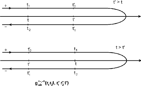
FIG. 1.: Time ordering on the Keldysh double time contour for the function $g_{ab}^{+-,-+}$. The ordering is causal on the upper branch and anticausal on the lower branch.

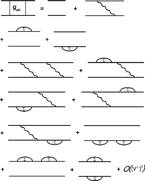
FIG. 2.: Diagrammatic expansion of the dynamically screened ladder equation up to second order.

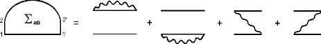
FIG. 3.: Diagramatic structure of the two-particle self-energy in first order in $V^{S}$.

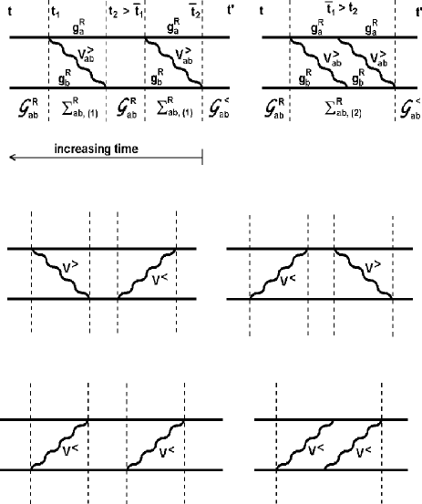
FIG. 4.: Evaluation of the ladder terms with two rungs. The first, the third, the fourth, and the fifth term are reducible, i.e., there are two successive self-energy insertions of first order. The second and the last term, however, are not reducible: they are two-particle self-energies of second order in $V^{S}$.

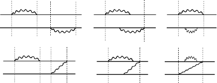
FIG. 5.: Here two other types of second-order terms are shown: in the first row two single-particle self-energies are combined, in the second row one single-particle self-energy is combined with one interaction between the particles. In dependence how the times do overlap, there are three different kinds of diagrams.

REFERENCES

- [1] L. Waldmann, Z. Naturforschung A 12, 660 (1957).
- [2] R. F. Snider, J. Chem. Phys. 32, 1051 (1960).
- [3] J. T. Lowry and R. F. Snider, J. Chem. Phys. 61, 2330 (1974).
- [4] J. A. McLennan, J. Stat. Phys. 28, 521 (1982).
- [5] S. Lagan and J. A. McLennan, Physica A 128, 178 (1984).
- [6] J. A. McLennan, J. Stat. Phys. 57, 887 (1989).
- [7] Y. L. Klimontovich and D. Kremp, Physica 109A, 517 (1981).
- [8] Y. L. Klimontovich, D. Kremp, and W. D. Kraeft, Adv. Chem. Phys. 68, 175 (1987).
- [9] W. Ebeling, W. D. Kraeft, and D. Kremp, Theory of Bound States and Ionization Equilibrium in Plasmas and Solids (Akademie–Verlag, Berlin, 1976).
- [10] W. D. Kraeft, D. Kremp, W. Ebeling, and G. Röpke, Quantum Statistics of Charged Particle Systems (Plenum, London, Akademie–Verlag, Berlin, 1986).
- [11] A. K. Rajagopal and C. K. Majumdar, J. of Mathematical and Physical Sciences 4, 109 (1970).
- [12] R. Zimmermann et al., phys. stat. sol. (b) 90, 175 (1978).
- [13] H. Haug and D. B. T. Thoai, phys. stat. sol.(b) 85, 561 (1978).
- [14] K. Shindo, J. Phys. Soc. Japan 29, 278 (1970).
- [15] M. Kilimann, D. Kremp, and G. Röpke, Theor. Mat. Fiz. 55, 448 (1983), [Theor. Mat. Phys. 55, 611 (1983)].
- [16] W. Schäfer and J. Treusch, Z. Phys. B - Condensed Matter 63, 407 (1986).
- [17] J. Seidel, S. Arndt, and W. D. Kraeft, Phys. Rev. E 52, 5387 (1995).
- [18] S. Arndt, W. D. Kraeft, and J. Seidel, phys. stat. sol. (b) 194, 601 (1996).
- [19] W. D. Kraeft et al., ApJ (1999), to appear in the May issue.
- [20] R. Zimmermann, Many-Particle Theory of Highly Excited Semiconductors (Teubner, Leipzig, 1988).
- [21] J. Dukelsky and P. Schuck, Nucl. Phys. A 512, 466 (1990).
- [22] S. Schaefer and P. Schuck, Phys. Rev. B 59, 1712 (1999).
- [23] W. Schäfer, R. Binder, and K. H. Schuldt, Z. Phys. B - Condensed Matter 70, 145 (1988).
- [24] D. Kremp, W. Kraeft, and M. Schlanges, in Strongly Coupled Coulomb Systems, edited by G. Kalman, J. Rommel, and K. Blagoev (Plenum Press, New York, 1998).
- [25] T. Bornath, Quantenstatistische Beschreibung dichter nichtidealer Plasmen im Nichtgleichgewicht, Habilitationsschrift, Universität Rostock, 1998, unpublished.
- [26] T. Bornath, M. Schlanges, and D. Kremp, Contrib. Plasma Phys. 39, 33 (1999), [Proceedings of the 9th International Workshop on the Physics of Nonideal Plasmas, Rostock 1998].
- [27] T. Bornath, The two-particle problem in a many-particle system: II. Nonequlibrium two-particle Dyson equation, 1999, to be published.
- [28] L. V. Keldysh, Zh. exp. teor. Fiz. 47, 1515 (1964), [Sov. Phys. JETP 20, 1018 (1965)].
- [29] D. F. DuBois, Lectures in Theoretical Physics (Interscience, New York, 1967), Vol. IXC, p. 469.
- [30] L. P. Kadanoff and G. Baym, Quantum Statistical Mechanics (Benjamin, New York, 1962).
- [31] J.-P. Blaizot and G. Ripka, Quantum Theory of finite systems (The MIT press, Cambridge(MA), London, 1986).
- [32] P. Danielewicz, Ann. Phys. (NY) 152, 239 (1984).
- [33] P. Danielewicz, Ann. Phys. (NY) 197, 154 (1990).
- [34] W. Botermans and R. Malfliet, Phys. Rep 198, 115 (1990).
- [35] E. M. Lifschitz and L. P. Pitajewski, Lehrbuch der Theoretischen Physik X: Physikalische Kinetik (Akademie–Verlag, Berlin, 1983).
- [36] H. Stolz, Einführung in die Vielelektronentheorie der Kristalle (Akademie–Verlag, Berlin, 1974).
- [37] G. H. Ecker and W. Weizel, Ann. Physik 17, 126 (1956).
- [38] M. Schlanges and T. Bornath, Physica A 192, 262 (1993).
- [39] T. Bornath and M. Schlanges, Physica A 196, 427 (1993).
- [40] M. Kilimann, W. D. Kraeft, and D. Kremp, Phys. Lett. A 61, 393 (1977).
- [41] D. B. Melrose and R. C. McPhedran, Electromagnetic processes in dispersive media (Cambridge University Press, Cambridge, 1991).
- [42] A. K. Rajagopal and M. H. Cohen, Journal of the Physical Society of Japan 26, suppl., 261 (1969).