Experimental evidence of a phase transition to fully developed turbulence in a wake flow
Abstract
The transition to fully developed turbulence of a wake behind a circular cylinder is investigated with respect to its statistics. In particular, we evaluated the probability density functions of velocity increments on different length scales . Evidence is presented that the -dependence of the velocity increments can be taken as Markov processes in the far field, as well as, in the near field of the cylinder wake. With the estimation of the deterministic part of these Markov processes, as a function of the distance from the cylinder, we are able to set the transition to fully developed turbulence in analogy with a phase transition. We propose that the appearing order parameter corresponds to the presence of large scale coherent structures close to the cylinder.
pacs:
turbulence - fluid dynamics 47.27; Fokker-Planck equation- stat. Physics 05.10G; Phase Transitions 05.70FI Introduction
In recent years considerable progress has been performed to understand the statistical features of fully developed, local isotropic turbulence [1]. Special interest has been addressed to understand intermittency effects of small scale velocity fluctuations characterized by the velocity increments at a scale . For most real flows these results are only applicable for small well defined regions of the flow, which may be regarded as local isotropic. A remaining challenge is to find out how theses concepts can help to understand real flows which are not fully developed or not homogeneous and isotropic [2].
The common method to characterize the disorder of fully developed local isotropic turbulence is to investigate the scale evolution of the probability density functions (pdf), , either directly or by means of their moments . Recently, it was found that this evolution can be related to a Markov process [3]. The Markovian properties can be evaluated thoroughly by investigating the joint and conditional pdfs, and , respectively [4]. From the conditional pdfs one can extract the stochastic equations, namely, the Kramers-Moyal expansion for the evolution of and the Langevin equation for [5]. This method provides a statistically more complete description of turbulence and furthermore assumptions, like scaling, are not needed, but can be evaluated accurately [3, 6].
In this work we present measurements of a turbulent flow behind a circular cylinder. The stochastic content of the velocity field as a function of the distance to the cylinder is investigated using the above mentioned Markovian approach. The main result, presented in this paper, is the finding of a phase transition like behavior to the state of fully developed turbulence. This phase transition characterizes the disappearance of the Karman vortices with respect to two parameters: the distance to the cylinder and the scale .
In the following we describe first the experimental set up. The measurements of longitudinal and transversal velocities are analyzed with respect to the dependent pdfs. Subsequently a test of Markov properties is presented. From the conditional pdf the first moment is evaluated. The coefficient reflects the deterministic part in the -evolution of the Markov process and can be taken to define an order parameter.
II experiment
Our work is based on hot-wire velocity measurements performed in a wake flow generated behind a circular cylinder inserted in a wind tunnel. Cylinders with two diameters of 2 cm and 5 cm were used. The wind tunnel [7] used has the following parameters: cross section 1.6m x 1.8m; length of the measuring section 2m; velocity 25m/s; residual turbulence level below 0.1 %. To measure longitudinal and transversal components of the local velocity we used x-wire probes (Dantec 55P71), placed at several distances, , between 8 and 100 diameters of the cylinder. The spatial resolution of the probes is about 1.5 mm.
From the measurements the following characteristic lengths were evaluated: the integral length, defined by the autocorrelation function, which varied between 10 cm and 30 cm depending on the cylinder used and location of the probe; the Kolmogorov length, was about 0.1mm; the Taylor length scale about 2.0 mm. Thus we see that our measurement resolved at least the turbulent structures down to the Taylor length scales. (Note, these lengths could be calculated precisely only for distances above 40 cylinder diameters.) The Reynolds numbers of these two flow situations were 250 and 650. Each time series consists of data points, and was sampled with a frequency corresponding to about one Kolmogorov length. To obtain the spatial variation the Taylor hypothesis of frozen turbulence was used.
III results
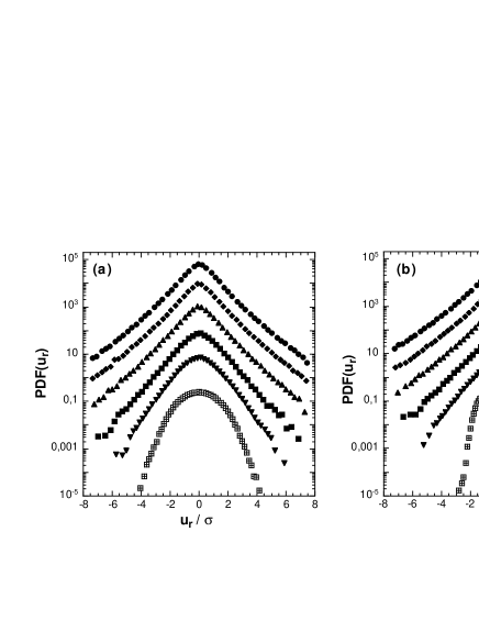
To investigate the disorder of the turbulent field the velocity increments for different scales and at different measuring points were calculated. Exemplary sequences of resulting pdfs are shown in Fig.1 for the transversal velocity component. In Fig. 1a the well known intermittency effect of isotropic turbulence is seen. At large scales nearly Gaussian distributions are present which become more and more intermittent (having heavy tailed wings) as the scale approaches the Kolmogorov length. Coming closer to the cylinder a structural change is found. Most remarkably a double hump pdf emerges for large . This structure reflects the fact that two finite values of the velocity increment are most probable. We interpret this as the result of counterrotating vortices passing over the detector. It should be noted that this effect was always found for the transversal velocity components. This is in consistency with the geometric features of vortices elongated parallel to the cylinder axis (Karman vortices). For small scales the humps vanish and the pdfs become similar to the isotropic ones.
IV Markov Process
Based on the findings that the evolution of the pdfs with for the case of fully developed turbulence can be described by a Fokker-Planck equation [3, 8], we apply the Markov analysis to the non fully developed states close to the cylinder. The basic quantity to be evaluated is the conditional pdf , where, , and is nested into by a midpoint construction. To verify the Markovian property, we evaluate the Chapman-Kolmogorov equation, c.f. [5]
| (1) |
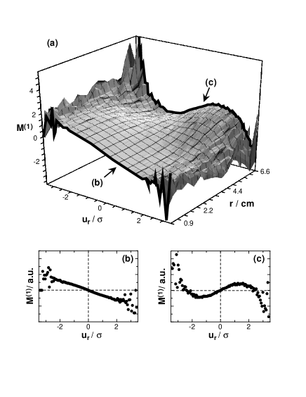
where . The validity of this equation was examined for many different pairs of . As a new result, we found that equation (1) also holds in the vicinity of the cylinder, i.e. in the non developed case of turbulence. For illustration see Figure 2; in part a the integrated conditional pdf (rhs of (1)) and the directly evaluated pdf (lhs of (1)) are shown by superimposed contour plots. In figurepart b three exemplary cut through these three dimensional presentations are shown. The quality of the validity of (1) can be seen from the proximity of the contour lines, or by the agreements of the conditional pdfs, represented by open and bold symbols [9]. Based on this result we treat the evolution of the statistics with the scale as a Markov process in . Thus the evolution of the pdf is described by the partial differential equation called Kramers-Moyal expansion [5]:
| (2) |
with the coefficients
| (3) | |||||
| (4) |
where . Notice, having once evaluated the conditional pdfs, these so called Kramers Moyal (KM) coefficients can be estimated directly from the data without any additional assumption. For our purpose it is sufficient to consider the for a small length of . The physical interpretation of the KM coefficients is the following: describes the deterministic evolution and is called drift term. , for reflect the influence of the noise. is called diffusion term. In the case of non Gaussian noise the higher order KM coefficients () become non zero.
We found that the structural change of the pdfs described above (see fig. 1) is mainly given by . As shown in figure 3, we find that close to the cylinder the form of the changes from a linear -dependence at small scales to a 3rd order polynomial behavior. From the corresponding Langevin equation [5] we know that the zeros of the drift term correspond to the fixed points of the deterministic dynamics. Fixed points with negative slope belong to accumulation points, having the tendency to build up local humps in the pdf. The change of the local slope of a fixed point (fig 3) can be set into correspondence to a phase transition, c.f. [10, 5]. Note that in contrast to other models, where the process evolves in time, here, we stress on the evolution in the scale variable .
The main point of our analysis is that we can determine the evolution equation in form of the KM coefficients. This tool is much more sensitive than merely looking at the pdfs or its moments, because the pdfs reflect only the transient behavior due to the underlying evolution equation. Thus it becomes clear that we are able to elaborate the phase transition even in the case where the double hump structure in the pdf may not be clearly visible. We want to mention that these double hump behavior of the pdfs can well be reproduced by calculating the stationary solution of the corresponding Fokker Planck equation, using our measured KM coefficient [11].
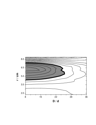
Beside the spatial scale parameter , the second parameter of the wake experiment is the distance of the probe to the cylinder. As it is well known, with increasing the distance a transition to fully developed turbulence takes place, i. e., the double hump structure vanishes. To characterize the phase transition in this two dimensional parameter space more completely we performed the above mentioned data analysis at several distances. As a criteria of a phase transition the local slope at was determined. The magnitude of this local slope is shown in figure 4 as a contour plot. The dark colored region reflects the parameter space, where 3 zeros for are present, or where the local slope at is positive. This is the region where the new order parameter exists. The critical line of the phase transition is marked by the bold black line.
V Discussion and Conclusion
We have presented a new approach to characterize also the disorder of not fully developed turbulence. The central aspect is that the disorder, described by velocity increments on different length scales, , are set into the context of Markov processes evolving in . Thus we can see how a given increment changes with decreasing due to deterministic and random forces. Both forces can be estimated directly from the data sets via Kramers-Moyal coefficients of the conditional probabilities. Most interestingly, we find significant changes in the deterministic force, the drift term, as one passes from non fully developed turbulence (close to the cylinder) into fully developed turbulence (far behind the cylinder). In the far field the drift term causes a stable fixed point at , i.e. the deterministic force causes a decrease of the magnitude of velocity increments as decreases. Approaching the near field at large this fixed point becomes instable, i.e. the slope of the drift term changes its sign at . In our one-dimensional analysis we find the appearance of two new stable (attracting) fixed point which are related to the double hump structure of the corresponding pdfs. This phenomenon may be set into relation with a phase transition, where the phase of the near field correspond to the existence of vortices. As the distance to the cylinder is increased these large scale structures vanish.
Finally some critical remarks are presented, to show in which direction work should be done in future. Visualizations indicate that even in the case of strong turbulence, the near field still resembles time periodic structures of counterrotationg vortex-like structures detaching from the cylinder, c.f. [12]. Theses time periodic large scale structures ask for a two-dimensional (two variable) modeling, in the sense of a noisy limit cycle. This apparent contradiction to our one-variable analysis, has to be seen on the background of the signal treatment. Applying to a time series the construction of increments (which represents a kind of high pass filter) the locality in time is lost. Thus also coherences in time may get lost, at least as long as one investigates small scale statistics. In this sense only a stochastic aspect of the counterrotating vortices is grasped. The challenge of a more complete characterization of the near field structures will require, in our opinion, a combination of increment analysis and real time modeling of the velocity data. At least for the ladder point a higher dimensional ansatz is required. Nevertheless we have presented in this work clear evidence how methods and results obtained from the idealistic case of fully developed turbulence can be used to characterize also the statistics in the transition region of a wake flow.
Acknowledgment: This work was supported by the DFG grant PE478/4. Furthermore we want to acknowledge the cooperation with the LSTM, namely, with T. Schenck, J. Jovanovic, F. Durst, as well as fruitful discussions with F. Chilla, Ch. Renner, B. Reisner and A. Tilgner.
REFERENCES
- [1] K.R. Sreenivasan, R.R. Antonia, Ann. Rev. Fluid Mech., 29 435 (1997); U. Frisch, Turbulence, Cambridge 1996
- [2] E. Gaudin, B. Protas, S. Goujon-Durand, J. Wojciechowski, J.E. Wesfreid, Phys. Rev. E, 57, R9 (1998); F. Chilla, J.F. Pinton, R. Labbe, Europhys. Lett. 35, 271 (1996); P.R. Van Slooten, Jayesh, S.B. Pope, Phys. Fluids 10, 246 (1998); P. Olla, Phys. rev E 57, 2824 (1998); .
- [3] R. Friedrich, J Peinke, Physica D 102 147 (1997); Phys.Rev.Lett. 78, 863 (1997)
- [4] R. Friedrich, J. Zeller, J. Peinke, Europhys. Lett. 41, 153 (1998)
- [5] c.f. P. Hänggi and H. Thomas, Physics Reports 88, 207 (1982); H. Risken, The Fokker-Planck equation, (Springer-Verlag Berlin, 1984).
- [6] J. Peinke, R. Friedrich, A. Naert, Z. Naturforsch 52 a, 588 (1997).
- [7] Wind tunnel of the Lehrstuhl für Strömungsmechanik, University of Erlangen, Germany, was used.
- [8] Ch. Renner, B. Reisner, St. Lück, J. Peinke, R. Friedrich, chao-dyn/9811019
- [9] It is known that the Chapman Kolmogorov equation is a necessary condition for the validity of a Markov process. There are only rare cases where the Chapman Kolmogorov equation holds when there is no Markov process present.
- [10] H. Haken, Synergetics (springen, Berlin 1983)
- [11] St. Lück et. al. to be published.
- [12] M. van Dyke, An Album of Fluid Motion (The Parabolic Press , Stanford 1982).