Coherent nuclear motion in a condensed-phase environment: Wave-packet approach and pump-probe spectroscopy

Abstract

A quantum-mechanical Gaussian wave-packet approach to the theoretical description of nuclear motions in a condensed-phase environment is developed. General expressions for the time-dependent reduced density matrix are given for a harmonic potential surface, and the exact quantum dynamics is found for a microscopic system-plus-bath model. Particular attention is devoted to the influence of initial correlations between system and bath for the outcome of a pump-probe experiment. We show that the standard factorized preparation, compared to a more realistic correlated preparation, leads to significantly different stimulated emission spectra at high temperatures. Recent experiments for the reaction center are analyzed using this formalism.

I Introduction

The notion of wave packets is intimately connected with the foundations of quantum mechanics itself. Despite of their importance during the initial stages of the development of quantum theory [1], this concept has been quickly overturned by the powerful and elegant operator formalism. Only during the past decade interest in wave packets has emerged again, primarily triggered by the widespread availability of ultrafast femtosecond laser pulse techniques [2]. Wave packets are by today a standard tool employed to explain many different features in chemistry and physics, e.g., chemical reaction dynamics [3, 4, 5], oscillatory motion of a coherent Bose-Einstein condensate [6], highly-excited Rydberg states in atoms [7], or electron-hole excitations in semiconductors [8, 9]. The concept of wave packets is sometimes applied to rationalize experimental data even though the reaction occurs under condensed-phase conditions, where the relevant reaction coordinate (e.g., describing the nuclear motion) of the wave packet (“system”) may be strongly coupled to other modes (“environment” or “bath”). At this point one may ask whether it makes sense to use a wave-packet description for the reaction coordinate dynamics even if strong coupling to solvent modes is present. First, the description of the wave packet in terms of a wavefunction is moot, and one has to use the reduced density matrix. Second, the bath leads to a damping of the wave packet and could cause the complete loss of coherence. In that case, the use of wave packets would be rather restricted. It is one of the purposes of this paper to clarify to what extent the wave-packet concept is applicable in the presence of strong system-bath coupling.

The dissipation acting on the wave packet can have many different microscopic origins. In gas-phase reactions, one typically has rather weak damping due to coupling to the vacuum modes of the electromagnetic field (spontaneous emission), or due to collisions with other molecules. In contrast, dissipation can become decisive in condensed-phase reactions where one has strong coupling of the system to solvent or protein polarization modes. Considering previous theoretical treatments of gas-phase reactions, dissipation was mostly ignored or at best incorporated within the framework of the Bloch equations [10] or the Redfield equations [11], where the latter allow to retain memory effects. However, as such an approach relies on perturbation theory in the system-bath coupling, its application to condensed-phase reactions characterized by strong system-bath coupling remains questionable. Other methods are based on classical molecular dynamics (MD) simulations [12] or projection operator techniques [5].

In general, the problem of dissipative wave-packet motion is theoretically quite demanding. In this paper, we treat a simple model introduced in Sections II and III but put particular emphasis on the effects due to different initial states of the system arising in pump-probe spectroscopy experiments. This issue is shown to be important for a correct description of experimental data on systems in a condensed-phase environment. More specifically, one might be tempted to assume a certain initial preparation which is named “factorized preparation” henceforth. Under the factorized preparation, the density matrix at $t=0$ factorizes into a system part describing the wave packet, and a part corresponding to the solvent modes. The wave packet at $t=0$ could then correspond to a pure state, e.g., a Gaussian wave packet. Here we provide a comparison of the factorized preparation to the more realistic “correlated preparation” which takes into account initial system-bath correlations [13]. We stress that such preparation effects cannot be captured by standard “dissipative wave-packet” approaches [3], which implicitely use the factorized preparation.

The structure of this paper is as follows. After presenting general expressions for Gaussian wave-packet dynamics in Sec. II, the connection to microscopic system-plus-environment models is established in Sec. III. In Sec. IV, we then consider a pump-probe spectroscopy experiment involving two harmonic surfaces. As a practical example, we analyze the recent stimulated emission experiments of the bacterial photosynthetic reaction center by Vos et al. [14, 15, 16], albeit the theory is more generally applicable. In that section, we also show that the two initial preparations mentioned above cause pronounced differences in the emission spectra at high temperatures. Finally, some conclusions are offered in Sec. V. Technical details have been deferred to an appendix.

II Gaussian density matrices

Let us start with general properties of the time evolution of a Gaussian reduced density matrix $\rho(t)$. The Gaussian property implies that the underlying Hamiltonian is at most quadratic in the system coordinate ($q$) and momentum ($p$), and imposes certain restrictions for the system-bath coupling. However, there is neither need to specify a Hamiltonian nor initial conditions for the system-bath complex at this stage [except consistency with the Gaussian form of $\rho(t)$]. The spatial representation of the density matrix reads

$$\rho(q,q^{\prime},t)=N^{-1}(t)\exp[-\Sigma(q,q^{\prime},t)]\;,$$ (1)

where $\Sigma(q,q^{\prime},t)$ denotes a quadratic form,

$$\Sigma(q,q^{\prime},t) = \frac{a_{1}}{4}q^{2}+\frac{a_{1}^{*}}{4}q^{\prime 2}-a_{2}q-a_{2}^{*}q^{\prime}+\frac{a_{3}}{2}qq^{\prime}$$ (2)

$$+ \frac{[a_{2}+a_{2}^{*}]^{2}}{a_{1}+a_{1}^{*}+2a_{3}}\;,$$ (3)

with arbitrary time-dependent coefficients $a_{i}(t)$. Furthermore, the normalization Tr$[\rho]=1$ is ensured by choosing

$\displaystyle N(t)=\sqrt{4\pi/[a_{1}+a_{1}^{*}+2a_{3}]}\;.$

While $a_{1}=a_{1}^{\prime}+ia_{1}^{\prime\prime}$ and $a_{2}=a_{2}^{\prime}+ia_{2}^{\prime\prime}$ can be complex-valued, $\rho=\rho^{\dagger}$ implies a real-valued coefficient $a_{3}$. Therefore we have five independent real-valued functions, and accordingly there are only five independent expectation values,

$$\langle q\rangle = 2a_{2}^{\prime}/[a_{1}^{\prime}+a_{3}]\;,$$

$$\langle p\rangle = \hbar\left(a_{2}^{\prime\prime}-\frac{a_{1}^{\prime\prime}a_{2}^{\prime}}{a_{1}^{\prime}+a_{3}}\right)\;,$$

$$\langle[\Delta q]^{2}\rangle = \frac{1}{a_{1}^{\prime}+a_{3}}\;,$$

$$\langle[\Delta p]^{2}\rangle = \frac{\hbar^{2}}{4}\left(a_{1}^{\prime}-a_{3}+\frac{a_{1}^{\prime\prime 2}}{a_{1}^{\prime}+a_{3}}\right)\;,$$

$$\langle[\Delta q,\Delta p]_{+}\rangle = -\hbar\frac{a_{1}^{\prime\prime}}{a_{1}^{\prime}+a_{3}}\;,$$

where $\Delta q=q-\langle q\rangle$, $\Delta p=p-\langle p\rangle$, and $[A,B]_{+}=AB+BA$.

Let us now assume that the Ehrenfest theorem holds. This implies

$$\frac{d}{dt}\langle q\rangle = \langle p\rangle/m\;,$$ (4)

$$\frac{d}{dt}\langle[\Delta q]^{2}\rangle = \langle[\Delta q,\Delta p]_{+}\rangle/m\;,$$ (5)

with the mass $m$. These equations eliminate two of the five degrees of freedom. Therefore we keep only $\langle q(t)\rangle$, the variance $\sigma(t)=2\langle[\Delta q]^{2}(t)\rangle$, and the quantity

$$\Theta(t)=\frac{2\hbar}{\sqrt{8\sigma\langle[\Delta p]^{2}\rangle-m^{2}\dot{\sigma}^{2}}}$$ (6)

as independent functions, where $\dot{\sigma}=d\sigma/dt$. The functions $a_{i}(t)$ can be expressed in terms of these three quantities, and Eq. (2) then takes the form

$${\rm Re}\,\Sigma(\langle q\rangle+Q,\langle q\rangle+Q^{\prime},t)=$$ (7)

$$\frac{1}{2\Theta^{2}\sigma}\left[\frac{1+\Theta^{2}}{2}(Q^{2}+Q^{\prime 2})-(1-\Theta^{2})QQ^{\prime}\right]\,,$$ (8)

$$\frac{\hbar}{m}\,{\rm Im}\,\Sigma(\langle q\rangle+Q,\langle q\rangle+Q^{\prime},t)=$$ (9)

$$Q^{\prime}\left(\frac{\dot{\sigma}Q^{\prime}}{4\sigma}+\frac{d\langle q\rangle}{dt}\right)-Q\left(\frac{\dot{\sigma}Q}{4\sigma}+\frac{d\langle q\rangle}{dt}\right)\;.$$ (10)

The normalization constant becomes simply $N=\sqrt{\pi\sigma}$. The real-valued quantity $\Theta$ is always within the bounds $0<\Theta(t)\leq 1$, with the limiting case $\Theta=1$ applying to a pure system. In fact, straightforward algebra yields

$$\Theta(t)={\rm Tr}\,[\rho^{2}(t)]\,.$$ (11)

It is noteworthy that $\Theta(t)$ is in general an independent quantity, as there is no Ehrenfest relation expressing $\langle[\Delta p]^{2}(t)\rangle$ solely in terms of $\langle q(t)\rangle$ and $\sigma(t)$.

By employing the unitary transformation

$$U(t)=\exp\left[-\frac{i}{\hbar}mq\left(\frac{\dot{\sigma}q}{4\sigma}+\frac{d\langle q\rangle}{dt}\right)\right]\exp\left[\frac{i}{\hbar}\langle q\rangle p\right]\;,$$ (12)

the density matrix $\widetilde{\rho}(t)=U\rho U^{\dagger}$ attains the coordinate-independent form

$$\widetilde{\rho}(t)=\widetilde{Z}^{-1}\exp(-\widetilde{\beta}\widetilde{H})\;,$$ (13)

with the Hamiltonian $\widetilde{H}(t)$ of a harmonic oscillator subject to an effective time-dependent confinement frequency

$$\widetilde{\Omega}(t)=\frac{\hbar}{m\sigma(t)\Theta(t)}\;.$$ (14)

The effective inverse temperature $\widetilde{\beta}$ is

$$\widetilde{\beta}(t)=\frac{1}{\hbar\widetilde{\Omega}(t)}\ln\left(\frac{1+\Theta(t)}{1-\Theta(t)}\right)\;,$$ (15)

and $\widetilde{Z}(t)=[2\sinh(\hbar\widetilde{\Omega}\widetilde{\beta}/2)]^{-1}$. The transformed density matrix (13) corresponds to the equilibrium density matrix of the harmonic oscillator $\widetilde{H}$ considered at fixed time $t$.

With the aid of this unitary transformation, it becomes easy to find the spectral decomposition of the density matrix. Transforming the result back to the original picture, we obtain

$$\rho(t)=\sum_{n=0}^{\infty}\lambda_{n}(t)|\varphi_{n}(t)\rangle\langle\varphi_{n}(t)|\;,$$ (16)

where the eigenvalues are given by

$$\lambda_{n}(t)=\frac{2\Theta}{1+\Theta}\left(\frac{1-\Theta}{1+\Theta}\right)^{n}\;.$$ (17)

The spatial representation of the eigenfunctions is

$$\varphi_{n}(Q+\langle q\rangle,t) = (\pi\sigma\Theta)^{-1/4}(2^{n}n!)^{-1/2}H_{n}(Q/\sqrt{\sigma\Theta})$$ (18)

$$\times \exp\left(\frac{i}{\hbar}\frac{m^{3}\dot{\sigma}(d\langle q\rangle/dt)^{2}}{8\langle[\Delta p]^{2}\rangle}\right)$$ (19)

$$\times \exp\left(-\frac{Q^{2}}{2\sigma\Theta}+\frac{imQ}{\hbar}\left[\frac{\dot{\sigma}Q}{4\sigma}+\frac{d\langle q\rangle}{dt}\right]\right)\;,$$ (20)

where $H_{n}$ are the usual Hermite polynomials. Transforming also $\widetilde{H}$ back into the original basis, we obtain

$$H(t)=\frac{(\Delta p-m\dot{\sigma}\Delta q/2\sigma)^{2}}{2m}+\frac{m\widetilde{\Omega}^{2}[\Delta q]^{2}}{2}\;.$$ (21)

In the end, the density operator can be written in the coordinate-independent form

$$\rho(t)=\widetilde{Z}^{-1}\exp\left(-\widetilde{\beta}(t)H(t)\right)\;.$$ (22)

Using Eq. (17), one readily checks that

$\displaystyle{\rm Tr}\,[\rho(t)]=\sum_{n=0}^{\infty}\lambda_{n}(t)=1\;,$

and similarly one recovers Eq. (11), since

$\displaystyle{\rm Tr}\,[\rho^{2}(t)]=\sum_{n}\lambda_{n}^{2}(t)=\Theta(t)\;.$

The linear entropy is then given by

$$S_{\rm lin}(t)\equiv 1-{\rm Tr}\,[\rho^{2}]=1-\Theta(t)\;,$$ (23)

and the Shannon entropy is

$$S(t) \equiv -{\rm Tr}\,[\rho\ln\rho]$$ (24)

$$= -\sum_{n}\lambda_{n}\ln\lambda_{n}$$ (25)

$$= \frac{1}{2}\ln\left(\frac{1-\Theta^{2}}{4\Theta^{2}}\right)+\frac{1}{2\Theta}\ln\left(\frac{1+\Theta}{1-\Theta}\right)\;.$$ (26)

III Microscopic system-plus-bath model

Let us now consider a wave packet moving in a harmonic potential surface under the influence of a bath composed of harmonic oscillators. The harmonic oscillator modes need not correspond to physical modes but could represent effective modes chosen to mimic the actual environment in an optimal way. Such a system-plus-bath model allows us to derive exact expressions for the independent expectation values $\langle q(t)\rangle$, $\sigma(t)$, and $\Theta(t)$ of Sec. II, and thereby to obtain the exact quantum dynamics of the damped wave packet for a given spectral density of the bath modes. In this section, the simpler case of a factorized preparation is treated. The correlated preparation is then discussed in Sec. IV B.

We study a system-plus-bath model [9], $H=H_{S}+H_{B}+H_{I}$, where the “system” part describing the undamped coherent nuclear motion reads

$$H_{S}=\frac{p^{2}}{2m}+\frac{m\omega_{0}^{2}}{2}(q-q_{0})^{2}\;.$$ (27)

The “bath” is composed of harmonic oscillators coupled linearly to the system coordinate,

$$H_{B}+H_{I}=\sum_{j}\left(\frac{p_{j}^{2}}{2m_{j}}+\frac{m_{j}\omega_{j}^{2}}{2}\left[x_{j}-\frac{c_{j}}{m_{j}\omega_{j}^{2}}q\right]^{2}\right)\;.$$ (28)

The influence of the bath onto the system is fully specified by the spectral density,

$$J(\omega)=\frac{\pi}{2}\sum_{j}\frac{c_{j}^{2}}{m_{j}\omega_{j}}\delta(\omega-\omega_{j})\;.$$ (29)

A frequently used model spectral density is given by the ohmic bath with a Drude cutoff [9],

$$J(\omega)=\frac{m\gamma\omega}{1+(\omega/\omega_{D})^{2}}\;.$$ (30)

Under the factorized preparation, the density matrix at time $t=0$ factorizes according to

$$\rho(t=0)=\rho_{S}(q)\otimes\rho_{B}(\{x_{j}\})\;.$$ (31)

Here $\rho_{S}(q)$ describes a pure Gaussian wave packet of width $\sigma_{0}$ centered around $q=0$, corresponding to the wavefunction

$\displaystyle\psi(q)=(\pi\sigma_{0})^{-1/4}\exp(-q^{2}/2\sigma_{0})\;.$

The bath is assumed to be in a thermal distribution, with the system coordinate held fixed at $q=0$. While equilibrium properties of a damped harmonic oscillator have been studied exhaustively in the past, the consideration of wave-packet initial preparations and their corresponding time evolution leaves room for our contribution.

Due to the harmonic nature of the total system-plus-bath complex, the exact time-dependent density matrix $\rho(q,q^{\prime},t)$ can then be directly obtained from Feynman-Vernon theory [9, 13]. Switching to symmetric and antisymmetric linear combinations,

$$x=(q+q^{\prime})/2\;,\quad y=q-q^{\prime}\;,$$ (32)

the propagating function of Ref.[13] immediately leads to the result

$$\rho(x,y,t) = \frac{1}{\sqrt{\pi\sigma}}\exp\Bigl{\{}-(x-\langle q\rangle)^{2}/\sigma-y^{2}/4\sigma\Theta^{2}$$ (33)

$$+ \frac{i}{\hbar}my\left(\frac{\dot{\sigma}(x-\langle q\rangle)}{2\sigma}+\frac{d\langle q\rangle}{dt}\right)\Bigr{\}}\;,$$ (34)

in accordance with the general form (1). Now the three independent expectation values can be expressed in terms of microscopic parameters,

$$\langle q(t)\rangle = \omega_{0}^{2}q_{0}\int_{0}^{t}dt^{\prime}\,G(t^{\prime})\;,$$ (35)

$$\sigma(t) = \sigma_{0}\dot{G}^{2}(t)+\frac{\hbar^{2}}{m^{2}\sigma_{0}}G^{2}(t)+\frac{2\hbar}{m^{2}}K_{q}(t)\;,$$ (36)

and $\Theta(t)$ is defined by Eq. (6) with

$$\langle[\Delta p]^{2}\rangle=\frac{m^{2}}{2}\left(\sigma_{0}\ddot{G}^{2}(t)+\frac{\hbar^{2}}{m^{2}\sigma_{0}}\dot{G}^{2}(t)+\frac{2\hbar}{m^{2}}K_{p}(t)\right)\;.$$ (37)

The definition of the functions $G(t)$, $K_{q}(t)$, and $K_{p}(t)$ for an arbitrary spectral density $J(\omega)$ can be found in the appendix. From these expressions, one verifies that the correct equilibrium values $\sigma_{\beta}$ and $\langle[\Delta p]^{2}\rangle_{\beta}$ [9] are approached at long times.

Using the ohmic spectral density (30), we now discuss the question of coherence of the damped wave packet. Above a critical value $\gamma_{c}$ of the damping strength $\gamma$, where $\gamma_{c}$ follows from Eq. (78), oscillations in $\langle q(t)\rangle$ disappear and only incoherent relaxation can take place, see Figure 1. For $\omega_{D}\gg\omega_{0}$, the critical damping strength is given by $\gamma_{c}=2\omega_{0}$ [9]. While this limit is of most interest in solid-state applications, the regime $\omega_{D}\approx\omega_{0}$ as well as $\omega_{D}\ll\omega_{0}$ has many applications in chemical systems. Interestingly, the value of $\gamma_{c}$ increases when $\omega_{D}/\omega_{0}$ becomes small. In fact, for $\omega_{D}\to 0$, the dynamics is always fully coherent, $\gamma_{c}=\infty$. In that limit, the bath is too slow to cause relaxational behavior. It is noteworthy that the precise value of $\gamma_{c}$ depends on the quantity considered in defining coherence. Taking the disappearance of the inelastic peaks in the spectral function as the relevant criterion leads to a critical value that is smaller by a factor $1/\sqrt{2}$ [17]. Since our coherence criterion is based

FIG. 1.: Critical damping strength $\gamma_{c}$ as a function of $\omega_{D}$ (solid curve). The limiting value $\gamma_{c}/2\omega_{0}=1$ for $\omega_{D}\gg\omega_{0}$ is indicated by the dashed line.

on the oscillatory behavior of $\langle q(t)\rangle$, where the latter equals the corresponding expression for a point-like particle, the coherent-to-incoherent transition occurs at the same damping strength $\gamma_{c}$ for a wave packet and a point-like particle. In particular, $\gamma_{c}$ takes a temperature-independent value.

Next we briefly discuss the time dependence of the variance $\sigma(t)$, see Figure 2, and of the Shannon entropy $S(t)$, see Figure 3. The initial width $\sigma_{0}$ of the wave packet

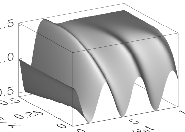
FIG. 2.: Variance $\sigma(t)$ as a function of $\gamma$ for $\hbar\beta\omega_{0}=1$, $\sigma_{0}=1.5\,\hbar/m\omega_{0}$, and $\omega_{D}/\omega_{0}=5$.

mainly influences the dynamics during the initial stage of the relaxation. Expanding for small times $\delta t$, the variance reads

$$\sigma(\delta t)\simeq\sigma_{0}+\left[\frac{\hbar^{2}}{m^{2}\sigma_{0}}-\sigma_{0}(\omega^{2}+\gamma\omega_{D})\right]\delta t^{2}\;.$$ (38)

Therefore the variance initially increases (decreases) for $\sigma_{0}<\tilde{\sigma}$ ($\sigma_{0}>\tilde{\sigma}$), where $\tilde{\sigma}=\hbar/m\sqrt{\omega_{0}^{2}+\gamma\omega_{D}}$. For $\gamma<\gamma_{c}$, oscillations in both $\sigma(t)$ and $S(t)$ are found, similar to the behavior of $\langle q(t)\rangle$. These oscillations again persist at high temperatures, albeit with smaller ampli-

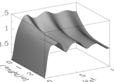
FIG. 3.: Shannon entropy $S(t)$ as a function of $\hbar\beta\omega_{0}$ for $\gamma/2\omega_{0}=0.1$, $\omega_{D}/\omega_{0}=15$, and $\sigma_{0}=1$.

tude. The initial entropy increase observed in Fig. 3 becomes very pronounced if $\sigma_{0}$ strongly deviates from the natural width $\sigma_{\beta}$ of the damped oscillator. Furthermore, initial transient oscillations then persist for a longer time. They are particularly pronounced for low temperatures and small $\sigma_{0}$, with a transient entropy large compared to the equilibrium value $S(t\to\infty)$.

IV Pump-probe spectroscopy of the Reaction Center

Next we apply the results presented before in a specific context. The system under study is the photosynthetic reaction center in purple bacteria. In recent pump-probe experiments on modified and wild-type reaction centers, Vos et al. [14, 15, 16] have observed oscillations in the time-resolved emission signal, which were interpreted to reflect coherent nuclear motion in the excited electronic state (“vibrational coherence”). This observation immediately received much attention, as coherent dynamics was not expected to exist in such a condensed-phase system. Clearly, a nuclear coordinate within a macromolecule like the reaction center could be drastically influenced by dissipation, which suggests a treatment similar to the one discussed above. The situation that Vos et al. constructed from their data is depicted in Fig. 4. The excited state surface was found to be parabolic with a curvature of $\omega_{0}=75\,{\rm cm}^{-1}$. It was populated with a 870 nm pump pulse, say, at time $t=0$, and probed with pulses around 921.5 nm, corresponding to the minimum of the excited state surface. In this section, we expand on the above analysis in order to describe the emission signal. Thereby effects of the spectral density characteristics and of the initial correlations can be captured, where especially the latter are missed by any simpler formalism. In order to clearly show these initial correlation effects, we shall crudely simplify the modelling of the pump (and to a lesser extent of the probe) pulse. In particular, we

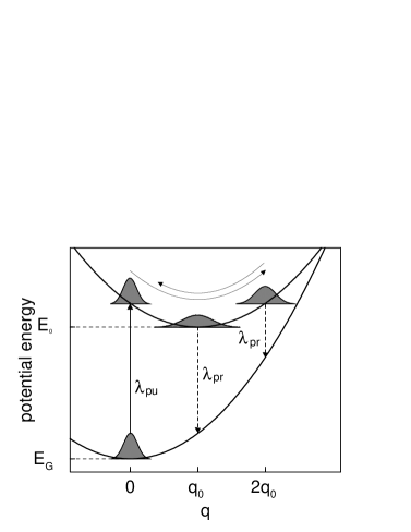
FIG. 4.: Pump-probe setup involving two harmonic surfaces. The dark (excited) state surface is centered at $q=0\;(q=q_{0})$.

make the (strictly speaking unphysical) assumption that the pump pulse transfers the complete nuclear wave packet up to the excited state surface. Therefore we only have to treat the dissipative excited state dynamics up to the probe pulse. Of course, thereby potentially important effects like the impulsive resonance Raman contribution [4, 5, 18] are missed. However, in principle our theory can straightforwardly be extended to provide a more realistic modelling of the pump and probe processes.

A Model and parameters

The Hamiltonian $H(t)=H_{0}+V(t)$ governing the emission process first consists of an unperturbed Hamiltonian

$$H_{0}=|G\rangle H_{G}\langle G|+|E\rangle(H_{E}+H_{I}+H_{B})\langle E|\;.$$ (39)

The orthonormal states $|G\rangle$ and $|E\rangle$ denote the electronic degrees of freedom, with $H_{G}$ ($H_{E}$) being the Hamiltonian in the ground (excited) state,

$$H_{G} = \frac{p^{2}}{2m}+\frac{m\omega_{G}^{2}}{2}q^{2}\;,$$

$$H_{E} = \frac{p^{2}}{2m}+\frac{m\omega_{0}^{2}}{2}(q-q_{0})^{2}+\hbar\omega_{\Delta}\;,$$

where $\hbar\omega_{\Delta}=E_{0}-E_{G}$ and $q_{0}$ is the separation of the potential minima, see Fig. 4. The dissipation acting on the wave packet in the excited state is included via $H_{I}+H_{B}$, see Eq. (28). Since we only consider the dynamics on the excited state surface between the pump and the probe pulse, it is not necessary to account for dissipation in the ground state at $t>0$. The effect of the probe pulse is described by $V(t)$. Under the dipole and the rotating wave approximation [5],

$$V(t)=\epsilon(t)|G\rangle\langle E|+\;{\rm H.c.}\;,$$ (40)

where $\epsilon(t)$ represents the temporal envelope of the electric field. The probe pulse was taken in the form

$$\epsilon(t^{\prime})=\theta[t^{\prime}-(t-\delta)]\,\theta[t+\delta-t^{\prime}]\,e^{i\omega_{pr}t^{\prime}}\;,$$ (41)

where $\theta$ is the Heaviside function and the probe pulse is centered at time $t$. Since the 30 fs probe pulses used in Ref. [14] did not maintain their full intensity over the whole pulse duration, we have chosen a smaller duration of $2\delta=20$ fs.

The model parameters were taken as follows. The frequency of the excited [ground] state surface is $\omega_{0}=75~{}{\rm cm}^{-1}$ [$\omega_{G}=130~{}{\rm cm}^{-1}$]. Furthermore, $q_{0}$ and $\hbar\omega_{\Delta}$ are calculated from the wavelength of the pump pulse, $\lambda_{pu}=870$ nm, and of the probe pulse acting at $q=q_{0}$, $\lambda_{pr}=921.5$ nm. The parabolic geometry of Fig. 4 then yields $q_{0}=2.07\sqrt{\hbar/m\omega_{0}}$ and $\omega_{\Delta}=11\,327$ cm^-1. At this point, little is known about microscopic details of the dissipation acting on the reaction coordinate $q$. In principle, one should first compute the appropriate spectral density for the system under consideration by means of MD simulations [19]. In the absence of such information, we make the assumption of an ohmic bath with a Drude cutoff, see Eq. (30). This spectral density was shown to be in agreement with the overall structure of the spectral density coupling to the primary electron transfer step in the reaction center [19]. To account for the lack of knowledge concerning the spectral density, we have studied two different spectral parameter sets. The first one, which is referred to as SP I, is $\gamma/2\omega_{0}=0.1$ and $\omega_{D}/\omega_{0}=100$. The second one, referred to as SP II, is $\gamma/2\omega_{0}=0.75$ and $\omega_{D}/\omega_{0}=0.5$. Both sets are within the coherent regime, $\gamma<\gamma_{c}(\omega_{D})$, and are chosen such that the oscillations in $\langle q(t)\rangle$ decay on the same time scale as those of the $T=10$ K emission signal reported in Ref. [14].

B Initial preparation

A conceptually more severe point concerns the proper description of the initial state ($t=0$). Again, two very different initial preparations are conceivable. The first one is to assume a wave packet in the usual sense, where the oscillator is initially in a pure state without correlations with the bath. This is the “factorized preparation” elaborated in Sec. III and (at least implicitely) employed in most previous treatments. On the other hand, the nuclear coordinate already experiences the environment while the system is in the ground state, and therefore the initial density matrix does not factorize. A more realistic preparation is to take the $|G\rangle$ oscillator at equilibrium with the same bath as in the excited state, whence there will be system-bath correlations at $t=0$ (“correlated preparation”). We mention in passing that the correlated preparation is related to the initial bath preparation discussed in Ref. [20] in the context of electron transfer reactions. The special case $\omega_{G}=\omega_{0}$ with $\omega_{D}\gg\omega_{0}$ has also been treated in Ref. [5] and references therein.

Due to its very short duration, as a result of the pump pulse at $t=0$, the system is assumed to suddenly change from the ground state to the excited state surface. This amounts to both a vertical shift and a change in curvature $\omega_{G}\rightarrow\omega_{0}$, see Fig. 4. Technically speaking, the correlated preparation can be most conveniently accounted for by following the path-integral analysis of Ref.[13], but keeping different system potentials acting on the imaginary-time and real-time paths. The resulting reduced density matrix is then of the form (33) again. Due to the Ehrenfest theorem, $\langle q(t)\rangle$ and $\langle p(t)\rangle$ coincide with the results of the factorized preparation. The variances $\sigma(t)$ and $\langle[\Delta p]^{2}(t)\rangle$ follow in closed form and are given in the appendix. For the corresponding results under the factorized preparation, see Eqs. (36) and (37).

For both preparations, the initial width $\sigma(t=0)$ was chosen as the thermal width $\sigma_{\beta}^{G}$ in the ground state oscillator. Importantly, despite of having the same initial value, the time-dependence of the variance is strikingly different depending on the initial condition. This becomes particularly evident for $\omega_{G}=\omega_{0}$, where for the correlated preparation, $\sigma(t)$ and $\langle[\Delta p]^{2}(t)\rangle$ stay constant in time, whereas the factorized preparation always leads to time-dependent variances. This can be understood by noting that $\langle[\Delta p]^{2}(t=0)\rangle$ for the factorized preparation is determined by the minimum uncertainty condition $\Theta(t=0)=1$, see Eq. (6), while it is given by $\langle[\Delta p]^{2}\rangle_{\beta}^{G}$, see Eq. (69), in the case of a correlated preparation. Since the deviation in $\langle[\Delta p]^{2}(t=0)\rangle$ for the two initial preparations becomes larger with increasing temperatures, one expects that the choice of the correct initial preparation is more important at high temperatures. This is indeed confirmed by the results for the stimulated emission signal reported below.

C Calculating the emission signal

Next we calculate the time-dependent total stimulated emission signal. After the pump pulse at $t=0$, the system is assumed to be in the excited state surface according to a properly chosen initial preparation. The probe pulse is then assumed to be much faster than typical solvent time scales such that the environmental influence can be neglected during the emission process itself. The time-dependent emission signal can thus be expressed in terms of the reduced density matrix directly before and after the application of the probe pulse. For a probe pulse centered at time $t$ with duration $2\delta$, the energy $E(t)$ emitted during the transition is

$$E(t) = \langle H_{0}\rangle_{\rho(t+\delta)}-\langle H_{0}\rangle_{\rho(t-\delta)}$$ (42)

$$= {\rm Tr}\{H_{0}[\rho(t+\delta)-\rho(t-\delta)]\}\;,$$ (43)

with the reduced density matrix $\rho(t)$. Herein the influence of the bath during the emission process has been neglected. Adopting a matrix representation for $\rho(t)$ with respect to the electronic states $|G\rangle$ and $|E\rangle$, we notice that $\rho(t^{\prime}<t-\delta)=|E\rangle\rho^{E}(t^{\prime})\langle E|$, since for $t^{\prime}<t-\delta$, the wave packet is located on the excited state surface. For $t^{\prime}>t-\delta$, however, $V(t^{\prime})$ causes a population of other matrix elements as well. Since we are interested in the emission signal, the trace in Eq. (42) allows us to focus only on the diagonal elements. Using second-order perturbation theory in $V(t)$, they read

$$\rho^{G}(t+\delta) = U_{1,GE}(t+\delta,t-\delta)\,\rho^{E}(t-\delta)$$ (44)

$$\times U_{1,EG}^{-1}(t+\delta,t-\delta)\;,$$ (45)

$$\rho^{E}(t+\delta) = U_{0}(t+\delta,t-\delta)\,\rho^{E}(t-\delta)\,U_{0}^{-1}(t+\delta,t-\delta)$$ (46)

$$+ \Big{[}U_{2}(t+\delta,t-\delta)\,\rho^{E}(t-\delta)\,U_{0}^{-1}(t+\delta,t-\delta)$$ (48)

$$\quad+\;{\rm H.c.}\Big{]}\;.$$

Here $U_{k}(t,t^{\prime})$ denotes the appropriate matrix element of the $k$th term of the Dyson expansion for the time evolution operator under $H(t)$,

$$U_{0}(t,t^{\prime}) = e^{-\frac{i}{\hbar}H_{E}(t-t^{\prime})}\,,$$

$$U_{1,EG}(t,t^{\prime}) = -\frac{i}{\hbar}\int_{t^{\prime}}^{t}dt_{1}\epsilon^{\ast}(t_{1})e^{-\frac{i}{\hbar}H_{E}(t-t_{1})}e^{-\frac{i}{\hbar}H_{G}(t_{1}-t^{\prime})}\,,$$

$$U_{2}(t,t^{\prime}) = -\frac{1}{\hbar^{2}}\int_{t^{\prime}}^{t}\,dt_{1}\int_{t^{\prime}}^{t_{1}}\,dt_{2}\,\epsilon(t_{1})\epsilon^{\ast}(t_{2})e^{-\frac{i}{\hbar}H_{E}(t-t_{2})}$$

$$\times e^{-\frac{i}{\hbar}H_{G}(t_{2}-t_{1})}e^{-\frac{i}{\hbar}H_{E}(t_{1}-t^{\prime})}\;,$$

with $U_{1,GE}(t,t^{\prime})=-U_{1,EG}^{\dagger}(t,t^{\prime})$. After some algebra, we obtain the time-resolved total emission signal in the form

$$E(t) = \frac{1}{\hbar}\,\sum_{n,r,s=0}^{\infty}\langle n|r\rangle\langle s|n\rangle\Bigg{(}2[\omega_{0}(s+1/2)+\omega_{\Delta}]$$ (49)

$$\times {\rm Re}\Big{\{}\rho_{rs}^{E}(t-\delta)e^{i\omega_{0}(r-s)(t-\delta)}$$ (50)

$$\times \int_{t-\delta}^{t+\delta}\,dt^{\prime}\,\epsilon(t^{\prime})\int_{t-\delta}^{t^{\prime}}\,dt^{\prime\prime}\,\epsilon^{\ast}(t^{\prime\prime})$$ (51)

$$\times \exp\{i\,[\omega_{G}(n+1/2)-\omega_{0}(r+1/2)-\omega_{\Delta}]t^{\prime}\}$$ (52)

$$\times \exp\{i\,[\omega_{0}(s+1/2)+\omega_{\Delta}-\omega_{G}(n+1/2)]t^{\prime\prime}\}\Big{\}}$$ (53)

$$- \omega_{G}\,(n+1/2)\rho_{rs}^{E}(t-\delta)e^{i\omega_{0}(r-s)(t-\delta)}$$ (54)

$$\times \int_{t-\delta}^{t+\delta}\,dt^{\prime}\,\epsilon(t^{\prime})\int_{t-\delta}^{t+\delta}\,dt^{\prime\prime}\,\epsilon^{\ast}(t^{\prime\prime})$$ (55)

$$\times \exp\{i\,[\omega_{G}(n+1/2)-\omega_{0}(r+1/2)-\omega_{\Delta}]t^{\prime}\}$$ (56)

$$\times \exp\{i\,[\omega_{0}(s+1/2)+\omega_{\Delta}-\omega_{G}(n+1/2)]t^{\prime\prime}\}\Bigg{)}\;,$$ (57)

where $|n\rangle$ and $|r,s\rangle$ denote the vibronic eigenstates of $H_{G}$ and $H_{E}$, respectively.

In principle, the above analysis can straightforwardly be extended in order to incorporate the pump pulse. The resulting initial reduced density matrix is then composed of four different contributions, namely those in Eq. (44) and the two nondiagonal terms. The subsequent time evolution with both electronic surfaces coupled to the bath could then be treated in a similar way as presented in Sec. III.

D Results for the reaction center

Figure 5 shows the time-resolved stimulated emission signal for different probe wavelengths $\lambda_{pr}$ at $T=10$ K. At such a low temperature, the difference between the factorized and correlated preparation is very small and can hardly be resolved in Fig. 5. The qualitative features of the emission signal can be understood within the wave-packet picture by relating $\lambda_{pr}$ to a particular value of the nuclear coordinate $q$, as is seen by plotting the discrete Fourier-transformed emission spectrum $A(\lambda_{pr})$ at the frequency $\tilde{\omega}$ corresponding to the ground oscillation, see Fig. 6. This frequency, determined from the imaginary part of the roots of Eq. (76), is 97.2 ${\rm cm}^{-1}$ for SP II but deviates less than 1% from $\omega_{0}$ for SP I. The maxima in $A(\lambda_{pr})$ then correspond to the left ($q=0$) and right ($q=2q_{0}$) turning points of the undamped nuclear wave-packet, while the minimum is related to the bottom of the potential surface $(q=q_{0})$ in Fig. 4. Due to the finite pulse duration and the different Franck-Condon overlap factors for $q>q_{0}$ and $q<q_{0}$, the corresponding value of $\lambda_{pr}$ differs from 921.5 nm, particularly at high temperatures. Since the turning points are passed once per period but the bottom is visited twice, the cor-

FIG. 5.: Emission signal $E(t)$ [in arbitrary units] for different probe wavelengths $\lambda_{pr}$ at $T=10$ K for the factorized preparation. The solid (dashed) curve is for SP I (SP II). For clarity, curves for subsequent values of $\lambda_{pr}$ have been shifted vertically.

responding emission signals should be oscillatory with frequency $\tilde{\omega}$ and $2\tilde{\omega}$, respectively [14]. This behavior is indeed found in Fig. 5. Focusing on SP I, the emission signal at $\lambda_{pr}=1000$ nm, corresponding to the right turning point, exhibits a phase shift of $\pi$ and a smaller amplitude compared to $\lambda_{pr}=870$ nm. This can be explained by noting that the right turning point is reached half a period later than the left one, whence the most significant initial contribution is damped more strongly. Apart

FIG. 6.: Emission spectrum $A(\lambda_{pr})$ [in arbitrary units] at $\tilde{\omega}$ for different temperatures. In (a) [(b)], we have taken SP I with a factorized [correlated] preparation. In (c) [(d)], we have taken SP II with a factorized [correlated] preparation.

from the decay of the oscillations in $E(t)$, damping of the nuclear motion is also reflected in a finite amplitude $A(\lambda_{pr})>0$ at the minimum. For wavelengths $\lambda_{pr}$ away from the turning points or the bottom, there are two different time intervals between subsequent passings of the transition region. This leads to the splitting of the maxima in the short-time emission signal observed in Fig. 5.

With increasing temperature, according to our argumentation above, the influence of the initial preparation should become more and more important. This is seen in the temperature dependence of the spectrum and of the emission signal shown in Figures 6 and 7, respectively. We first focus on the effects seen in Fig. 6. The minimum of $A(\lambda_{pr})$ shifts towards higher wavelengths with increasing temperature. This can be rationalized by noting that for $\omega_{0}<\omega_{G}$, the energy gap between the $n$th vibronic eigenstates of the excited and ground state decreases with $n$, and that high-order eigenstates become more important in the spectral decomposition of $\rho(t)$ at

FIG. 7.: Emission signal $E(t)$ for $\lambda_{pr}=950$ nm and several temperatures for (a) SP I and (b) SP II. The solid (dashed) curve is for the correlated (factorized) preparation. Curves for subsequent temperatures have been shifted vertically by the same amount.

higher temperatures. In fact, additional calculations for $\omega_{G}=\omega_{0}/2$ [not shown here] yield a similar shift towards smaller $\lambda_{pr}$. This shift is more pronounced for the correlated initial preparation, but depends only weakly on the spectral density of the environmental modes.

Figure 7 shows the temperature dependence of the emission signal at $\lambda_{pr}=950$ nm, corresponding to $q_{0}<q<2q_{0}$, with $q$ approaching the bottom $q=q_{0}$ as the temperature is increased. Furthermore, Figure 8 shows that $\sigma(t)$ under the factorized preparation experiences a phase shift of almost $\pi$ at $T>100$ K compared to the correlated preparation. Such an unphysical phase shift arises as a relict of the unperturbed evolution of a harmonic oscillator. Furthermore, since $\sigma(0)=\sigma_{\beta}^{G}$ increases with temperature, a negative initial slope results under the factorized preparation, see Eq. (38). Notably, for the correlated preparation, the maxima in $E(t)$ stay always close to the equilibrium values, in marked contrast to the factorized preparation but in accordance with the experimental data of Ref. [14]. A similar behavior is seen in the variance shown in Fig. 8. For the correlated preparation, the maxima in $\sigma(t)$ occur every $(k+1/2)$th period, corresponding to the passing of the bottom $q=q_{0}$, and they are very close to their equilibrium value $\sigma_{\beta}^{E}$. Therefore, for the correlated preparation, the independent expectation values $\langle q(t)\rangle$ and $\sigma(t)$ are always close to their equilibrium values when passing the bottom $q=q_{0}$. On the other hand, for the factorized preparation, the phase shift in $\sigma(t)$ results in a bunching of the wave packet when passing the bottom. This causes even qualitatively different emission signals. We conclude that at high temperatures several unphysical effects are introduced by using a factorized initial preparation, and a wrong description of the emission spectrum may result.

FIG. 8.: Temperature dependence of $\sigma(t)$ [in units of $\tilde{\sigma}_{E}=\hbar/m\sqrt{\omega_{0}^{2}+\gamma\omega_{D}}$] for (a) SP I and (b) SP II. The solid (dashed) curve is for the correlated (factorized) preparation.

V Conclusions

In this work, we have formulated a dissipative wave-packet approach towards a detailed theoretical description of stimulated emission pump-probe experiments under condensed-phase conditions. Assuming harmonic surfaces for both the ground and the excited state, the Gaussian nature of the wave packet describing the coherent nuclear motion allows for an exact treatment even if strong damping by environmental modes is present. Modelling the environmental modes by a set of infinitely many effective harmonic oscillators with a suitably chosen spectral density, it is then possible to make detailed predictions for the stimulated emission signal and for the corresponding spectra. While the spectral density is in principle accessible in terms of MD simulations, we have studied two model spectral densities in this work. A particular advantage of our approach is the possibility of treating different initial preparations of the wavepacket-plus-bath complex directly after the pump pulse ($t=0$). A more realistic calculation should also explicitely study the pump pulse, which can in principle be done along the same lines. Under such a formalism, a correct choice for the initial preparation of the wavepacket-plus-bath complex before the pump pulse will be important and is expected to lead to similar effects.

The recent experiments by Vos et al. [14, 15, 16] on the bacterial photosynthetic reaction center have been analyzed using this formalism. Due to our assumptions about the pump pulse, the possibly important impulsive resonant Raman contribution was not taken into account here. While some of the qualitative features of the coherent nuclear motion have been discussed before using simpler arguments [14], our approach can allow for a fully quantum-mechanical comparison of experimental data with theory. Even in the absence of detailed knowledge about the environmental spectral density, conclusions of relevance to the interpretation of experimental results can be extracted from our analysis. In particular, we have shown that at high temperatures, the assumption of a factorized initial state leads to large differences from the theoretical predictions under a more realistic correlated initial state.

Finally it should be stressed that the approach presented here can be applied to other pump-probe spectroscopy setups as well. In particular, if the excited state surface is weakly coupled to another surface, as happens, e.g., in the primary electron transfer step in the reaction center, transitions to this surface are expected to modify the emission signal. A theoretical description of such a situation can be given in terms of spin-boson type models [20] and will be elaborated elsewhere.

Variances

This appendix contains the expressions for the variances appearing in the general reduced density matrix (33). Depending on the initial preparation, we get different results as described below.

For a factorized preparation, the three independent expectation values are given by Eqs. (35-37). The various quantities appearing therein read as follows. For a specific spectral density $J(\omega)$, the bath correlation function is

$\displaystyle L(t)=\frac{1}{\pi}\int_{0}^{\infty}d\omega\,J(\omega)\{{\rm coth}(\omega\hbar\beta/2)\cos(\omega t)-i\sin(\omega t)\}\;,$

and the Laplace-transformed damping kernel reads,

$$\hat{\gamma}(z)=\frac{2z}{\pi m}\int_{0}^{\infty}d\omega^{\prime}\,\frac{J(\omega^{\prime})}{\omega^{\prime}}\frac{1}{\omega^{\prime 2}+z^{2}}\;.$$ (58)

The functions $K_{q}(t)$ and $K_{p}(t)$ are defined as

$$K_{q}(t) = \int_{0}^{t}dt^{\prime}\,G(t^{\prime})\int_{0}^{t}dt^{\prime\prime}\,G(t^{\prime\prime})L^{\prime}(t^{\prime}-t^{\prime\prime})\;,$$ (59)

$$K_{p}(t) = \int_{0}^{t}dt^{\prime}\,\dot{G}(t^{\prime})\int_{0}^{t}dt^{\prime\prime}\,\dot{G}(t^{\prime\prime})L^{\prime}(t^{\prime}-t^{\prime\prime})\;,$$ (60)

with $L^{\prime}(t)=\,{\rm Re}L(t)$ and $G(t)$ being the inverse Laplace transform of

$$\hat{G}(z)=\left[z^{2}+z\hat{\gamma}(z)+\omega_{0}^{2}\right]^{-1}\;.$$ (61)

In order to ensure that the wave packet relaxes to $q=q_{0}$ at long times, the bath must fulfill the condition $G(t\to\infty)=0$. Otherwise it merely leads to a mass renormalization but not to truly dissipative behavior.

To obtain the time-dependent variances (36) and (37) in practice, it is necessary to find a more convenient form of Eqs. (59) and (60). By following Ref. [13], we obtain ($\nu_{n}=2\pi n/\hbar\beta$)

$$K_{q}(t) = \frac{m}{\hbar\beta}\Bigl{[}2\sum_{n=0}^{\infty}\Bigl{\{}\left(1-\hat{G}^{-1}(\nu_{n})\int_{0}^{t}dt^{\prime}\,G(t^{\prime})e^{-\nu_{n}t^{\prime}}\right)$$ (62)

$$\times \int_{0}^{t}dt^{\prime}\,G(t^{\prime})e^{\nu_{n}t^{\prime}}-G^{2}(t)+\int_{0}^{t}dt^{\prime}\,G(t^{\prime})e^{-\nu_{n}t^{\prime}}\Bigr{\}}$$ (63)

$$- \Bigl{\{}\left(2-\omega_{0}^{2}\int_{0}^{t}dt^{\prime}\,G(t^{\prime})\right)\int_{0}^{t}dt^{\prime}\,G(t^{\prime})\Bigr{\}}\Bigr{]}$$ (64)

and

$$K_{p}(t) = \frac{m}{\hbar\beta}\Bigl{[}2\sum_{n=0}^{\infty}\Bigl{\{}\left(\nu_{n}-\hat{G}^{-1}(\nu_{n})\int_{0}^{t}dt^{\prime}\,\dot{G}(t^{\prime})e^{-\nu_{n}t^{\prime}}\right)$$ (65)

$$\times \int_{0}^{t}dt^{\prime}\,\dot{G}(t^{\prime})e^{\nu_{n}t^{\prime}}-\nu_{n}\int_{0}^{t}dt^{\prime}\,\dot{G}(t^{\prime})e^{-\nu_{n}t^{\prime}}$$ (66)

$$- \dot{G}^{2}(t)+1\Bigr{\}}+\omega_{0}^{2}G^{2}(t)\Bigr{]}\;.$$ (67)

For $t\to\infty$, the equilibrium variances then follow as

$$\sigma_{\beta} = \frac{2}{m\beta}\sum_{n=-\infty}^{\infty}\hat{G}(|\nu_{n}|)\;,$$ (68)

$$\langle[\Delta p]^{2}\rangle_{\beta} = \frac{m}{\beta}\sum_{n=-\infty}^{\infty}[1-\nu_{n}^{2}\hat{G}(|\nu_{n}|)]\;.$$ (69)

For the correlated preparation discussed in Sec. IV B, while $\langle q(t)\rangle$ stays the same as under the factorized preparation, the variances now read

$$\sigma(t) = \frac{2\hbar}{m}\Bigl{(}\Lambda_{G}\dot{G}^{2}(t)+\Omega_{G}G^{2}(t)+B(t)$$ (70)

$$+ 2\Bigl{\{}\Lambda_{G}\dot{G}(t)\,G(t)\,C_{1}^{+}(t)-G^{2}(t)\,C_{2}^{+}(t)\Bigr{\}}$$ (71)

$$+ \frac{1}{m}K_{q}(t)\Bigr{)}\;,$$ (72)

$$\langle[\Delta p]^{2}\rangle(t) = \hbar m\Bigl{(}\Lambda_{G}\ddot{G}^{2}(t)+\Omega_{G}\dot{G}^{2}(t)+S(t)$$ (73)

$$+ 2\Bigl{\{}\Lambda_{G}\ddot{G}(t)\bar{C}_{1}(t)-\dot{G}(t)\bar{C}_{2}(t)\Bigr{\}}+\frac{1}{m}K_{p}(t)\Bigr{)}\;.$$ (74)

Herein the various quantities are given as follows [13],

$$\Omega_{G} = \frac{1}{\hbar\beta}\sum_{n=-\infty}^{\infty}\hat{G}_{G}(|\nu_{n}|)(\omega_{G}^{2}+|\nu_{n}|\hat{\gamma}(|\nu_{n}|))\;,$$

$$\Lambda_{G} = \frac{1}{\hbar\beta}\sum_{n=-\infty}^{\infty}\hat{G}_{G}(|\nu_{n}|)\;,$$

$$B(t) = \frac{1}{\hbar\beta}\sum_{n=-\infty}^{\infty}\hat{G}_{G}(|\nu_{n}|)\int_{0}^{t}ds\int_{0}^{t}du\;[g_{n}(s)g_{n}(u)$$

$$- f_{n}(s)f_{n}(u)]G(t-s)G(t-u)\;,$$

$$S(t) = \frac{1}{\hbar\beta}\sum_{n=-\infty}^{\infty}\hat{G}_{G}(|\nu_{n}|)\int_{0}^{t}ds\int_{0}^{t}du\;[g_{n}(s)g_{n}(u)$$

$$- f_{n}(s)f_{n}(u)]\dot{G}(t-s)\dot{G}(t-u)\;,$$

where $\hat{G}_{G}$ is given by Eq. (61) with $\omega_{0}$ being replaced by $\omega_{G}$. The functions $g_{n}$ and $f_{n}$ are given by

$$g_{n}(s) = \frac{1}{m\pi}\int_{0}^{\infty}d\omega\,J(\omega)\frac{2\omega}{\omega^{2}+\nu_{n}^{2}}\,\cos(\omega s)\;,$$

$$f_{n}(s) = \frac{1}{m\pi}\int_{0}^{\infty}d\omega\,J(\omega)\frac{2\nu_{n}}{\omega^{2}+\nu_{n}^{2}}\,\sin(\omega s)\;.$$

Furthermore, we have used the abbreviations

$$C_{1}(s) = \frac{1}{\hbar\beta\Lambda_{G}}\sum_{n=-\infty}^{\infty}\hat{G}_{G}(|\nu_{n}|)g_{n}(s)\;,$$

$$C_{2}(s) = \frac{1}{\hbar\beta}\sum_{n=-\infty}^{\infty}\hat{G}_{G}(|\nu_{n}|)\nu_{n}f_{n}(s)\;,$$

$$C_{i}^{+}(t) = \int_{0}^{t}ds\;C_{i}(s)\frac{G(t-s)}{G(t)}\;,$$

$$\bar{C}_{i}(t) = \int_{0}^{t}ds\;C_{i}(s)\dot{G}(t-s)\;.$$

Next we briefly discuss the case of an ohmic bath with a Drude cutoff, see Eq. (30). The damping kernel then exhibits exponential decay, $\gamma(t)=\gamma\omega_{D}\exp[-\omega_{D}t]$, with the Laplace transform

$$\hat{\gamma}(z)=\frac{\gamma\omega_{D}}{\omega_{D}+z}\;.$$ (75)

Defining $\lambda_{i}$ for $i=1,2,3$ as the roots of the cubic equation

$$z^{3}-\omega_{D}z^{2}+(\gamma\omega_{D}+\omega_{0}^{2})z-\omega_{0}^{2}\omega_{D}=0\;,$$ (76)

one obtains [21]

$$\hat{G}(z)=\frac{z+\omega_{D}}{(z+\lambda_{1})(z+\lambda_{2})(z+\lambda_{3})}=\sum_{i=1}^{3}\frac{\Lambda_{i}}{z+\lambda_{i}}\;,$$ (77)

where the coefficients $\Lambda_{i}$ follow as

$\displaystyle\Lambda_{i}=\frac{\lambda_{i}(\omega_{D}-\lambda_{i})}{2\lambda_{i}^{3}-\omega_{D}(\lambda_{i}^{2}-\omega_{0}^{2})}\;.$

From Eq. (77) we arrive at the simple result $G(t)=\sum_{i}\Lambda_{i}\exp[-\lambda_{i}t]$. All variances can then be evaluated in closed form [22]. As the resulting expressions are very lengthy but can be straightforwardly obtained by following the above steps, we refrain from quoting them here.

To locate the coherent-to-incoherent transition, we note that the cubic equation (76) has either three real solutions, or one real and two complex conjugate ones. In the latter case, $G(t)$ and therefore $\langle q(t)\rangle$ will exhibit coherent oscillations. The critical value $\gamma_{c}$ then follows from the condition $D(\bar{\gamma},\bar{\omega}_{D})=0$, where $\bar{\gamma}=\gamma/\omega_{0}$, $\bar{\omega}_{D}=\omega_{D}/\omega_{0}$, and

$$D(\bar{\gamma},\bar{\omega}_{D}) = \bar{\gamma}^{3}+\bar{\gamma}^{2}\left(\frac{3}{\bar{\omega}_{D}}-\frac{\bar{\omega}_{D}}{4}\right)$$ (78)

$$+ \bar{\gamma}\left(\frac{3}{\bar{\omega}_{D}^{2}}-5\right)+\frac{1}{\bar{\omega}_{D}^{3}}+\frac{2}{\bar{\omega}_{D}}+\bar{\omega}_{D}\;.$$ (79)

For arbitrary $\omega_{0}$ and $\omega_{D}$, there is exactly one positive value $\gamma=\gamma_{c}$ solving the condition $D=0$.

REFERENCES

[1] E. Schrödinger, Ann. Phys. 79, 489 (1926).
[2] G. Beddard, Rep. Prog. Phys. 56, 63 (1993);
A.H. Zewail, J. Phys. Chem. 97, 12427 (1993).
[17] R. Egger, H. Grabert, and U. Weiss,
Phys. Rev. E 55, R3809 (1997).
[18] B. Wolfseder et al., Chem. Phys. 233, 323 (1998).
[19] M. Marchi, J.N. Gehlen, D. Chandler, and M.J. Newton,
J. Am. Chem. Soc. 115, 4178 (1993).
[20] A. Lucke, C.H. Mak, R. Egger, J. Ankerhold, J. Stockburger,
and H. Grabert, J. Chem. Phys. 107, 8397 (1997).
[21] R. Karrlein and H. Grabert, Phys. Rev. E 55,
153 (1997).
[22] L. Mühlbacher, Diploma thesis (University of
Freiburg, 1998, unpublished).