On the El-Niño Teleconnection to Spring Precipitation in Europe

Abstract

In a statistical analysis of more than a century of data we find a strong connection between strong warm El Niño winter events and high spring precipitation in a band from Southern England eastwards into Asia. This relationship is an extension of the connection mentioned by Kiladis and Diaz (1989), and much stronger than the winter season teleconnection that has been the subject of other studies. Linear correlation coefficients between DJF NINO3 indices and MAM precipitation are higher than $r=0.3$ for individual stations, and as high as $r=0.49$ for an index of precipitation anomalies around 50^∘N from 5^∘W to 35^∘E. The lagged correlation suggests that south-east Asian surface temperature anomalies may act as intermediate variables.

1 Introduction

The recent strong El Niño has stirred up again interest in possible teleconnections to Europe. A few influences have been mentioned in previous studies. During the winter season, Scandinavia was found to be colder and dryer just after cold (La Niña) events (Berlage, 1966), and an increase in temperature and precipitation with El Niño conditions was found in this area (van Loon and Madden, 1981; Halpert and Ropelewski, 1992). Central European winters would have the opposite tendencies: warmer and wetter (Kiladis and Diaz, 1989) during ENSO warm events; this squares with the increase of cyclonic Großwetter days observed in Germany (Fraedrich, 1994) and England (Wilby, 1993) during El Niño years.

For the spring season after an El Niño event (Kiladis and Diaz, 1989) note precipitation anomalies in central Europe, and (Halpert and Ropelewski, 1992) find temperature anomalies in South-western Europe and Northern Africa.

Recently, new data sets of historical data have become available. This has opened up the possibility to check existing conjectures at higher statistical significance levels. This study was initiated by a search for an ENSO influence in the Netherlands through tropical storm activity. Tropical storm and hurricane activity on the Atlantic is suppressed by El Niño (Gray, 1984), and many catastrophic downpours in De Bilt are remnants of tropical storms during the Atlantic hurricane season. Unfortunately, this does not lead to an observable anti-correlation between the NINO3 index and precipitation (or high-precipitation events).

In this article we present a new analysis of the strongest statistical connection between ENSO and the weather in Europe we did find: increased spring precipitation after an El Niño event. In section 2 we detail the connection for one station, De Bilt in the Netherlands. The relationship is extended over Europe in section 3, and we search for possible mechanisms in section 4.

2 Rain in De Bilt

Two years ago we noticed that there was a correlation between the strength of an El Niño, quantified by the NINO3.4 index and spring (MAM) precipitation in De Bilt (central Netherlands) using data from 1950 to 1995. With a 3-month lag the linear correlation coefficient was 0.30, with a nominal significance of 95%. Given that we had considered more than 24 possible relationships, this result was not very convincing. It hinged on one extreme event: in 1983 the spring had been extraordinarily wet (see Fig. 1). Recently we used the precipitation series back to 1849 and forward to 1998 including a few more strong El Niño events. Also, Kaplan et al. (1998) give a reconstruction of the NINO3 index from 1856 to 1991. It uses only sea surface temperature (SST) measurements, and correlates quite well with the Jakarta SO index of Können et al. (1998): $r=0.66$ in DJF and $0.67$ in MAM over 133 years in 1859–1996. From 1950 onwards we use the NCEP analyses (Reynolds and Smith, 1994), over the overlap period the correlation with the Kaplan NINO3 is $0.97$. An analysis using the standard SO index (Allan et al., 1991; Können et al., 1998) gives essentially the same results.

Figure 1 shows that the relationship between the winter (DJF) NINO3 index and spring (MAM) precipitation in De Bilt was confirmed in the new analysis. The linear correlation coefficient is $r=0.35$, nominally this has a chance $P<10^{-4}$ of being random. The average of the four Dutch stations with data from 1867 (De Bilt, Groningen, Den Helder and Hoofddorp) gives a correlation of $0.40$.

Figure 1: A scatter plot of spring (MAM) precipitation in De Bilt, Netherlands versus the NINO3 index of SST in the eastern Pacific for 1857–1998. Underlined numbers refer to the 19th century. The horizontal thin lines give the 10%, 33%, 67% and 90% percentiles.

Figure 2: Mean and $2\sigma$ uncertainties of the precipitation in De Bilt for the years with $N_{3}>N_{3}^{\mathrm{cut}}$ (dashed curves), and $N_{3}<N_{3}^{\mathrm{cut}}$ (solid curves).

To quantize the significance of these relationships we used a Kolmogorov-Smirnov test to compute the probability that the precipitation distribution with NINO3 index $N_{3}<N_{3}^{\mathrm{cut}}$ is the same as the one with $N_{3}>N_{3}^{\mathrm{cut}}$. The averages and $2\sigma$ bands of these distributions of the De Bilt data are shown in Figure 2. The difference is significant at the 99% level for $N_{3}^{\mathrm{cut}}>0.5$: an El Niño tends to be followed by a wet spring. On the other hand, the effects of La Niña, including the suggestive drought in 1893, are not significant even at the 95% confidence level at De Bilt. For the four-station average this difference is also significant at the 95% level for $N_{3}^{\mathrm{cut}}<-0.5$.

The signal has no connection with the North Atlantic Oscillation (NAO). On the one hand the NAO does not influence precipitation in the Netherlands very much, on the other hand ENSO and NAO are only correlated in the summer.

3 Spring rain in Europe

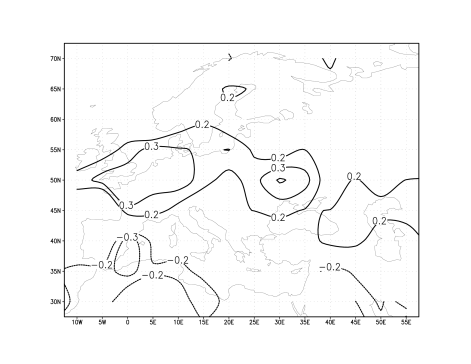
Figure 3: The linear correlation coefficients of the DJF NINO3 index and the MAM precipitation over Europe (1857–1993).

We investigated the extent of the teleconnection using the NCDC gridded precipitation anomalies database (Baker et al., 1995). This contains global data from 1851 to 1993 in 5^∘$\times$5^∘ bins. In Figure 3 one sees that the spring precipitation increases after an El Niño in a zonal belt from England and France to the Ukraine, with a weaker extension eastwards into Asia. There are two maxmima, with correlations coefficients above $0.3$ (without the 1998 El Niño): southern England, northern France, the Low Countries and Germany, and another one in the Ukraine centered on Kiev ($r=0.43$). This last point was also noted by Kiladis and Diaz (1989). In their Fig. 3h a similar but more southerly band is indicated over Europe. This band forms a dipole with the drier zone over Northern Africa and eastern Spain ($r=-0.35$), also noted in Kiladis and Diaz (1989). In contrast, the correlation of DJF precipitation with the DJF NINO3 index only reaches values above $0.2$ in three grid points: $0.22$ in Brussels, $0.23$ in Moscow and $-0.29$ in Bergen, Norway; none of these reach 99% significance. The Iberian signals in the summer and early fall are also weaker.

Figure 4: Scatter plot of the MAM precipitation anomalies in Europe around 50^∘N against the DJF NINO3 index for 1857–1993.

The relation with ENSO is seen more clearly when we construct an index of average MAM rainfall anomalies over the band with positive correlations consisting of the nine 5^∘$\times$5^∘ grid boxes centered on 50^∘N from 5^∘W to 35^∘E. This index has a correlation coefficient with DJF NINO3 of $r=0.49$, and one can see from figure 5 that the effect now looks significant for all values of $N_{3}$. A K-S test confirms that the distributions are different for the entire range of cut-off values. The correlation with the NAO is again low, although non-zero ($r=-0.16$).

Figure 5: Mean and $2\sigma$ uncertainties of the precipitation anomaly around 50^∘N from 5^∘W to 35^∘E. Dashed curves: the years with $N_{3}>N_{3}^{\mathrm{cut}}$, solid curves: below $N_{3}<N_{3}^{\mathrm{cut}}$.

4 Possible mechanisms

Figure 6: Lag correlation coefficients of the precipitation in spring and winter in De Bilt and in Europe around 50^∘N with the NINO3 index.

Possible mechanisms of this teleconnection have to explain the time structure of the correlation. The lag correlations of the MAM precipitation with the NINO3 index is shown in figure 6. For reference we also show the DJF correlations. Although there is room for an atmospheric mechanism with a time scale shorter than a month, the main signal seems to be delayed by 3–6 months. This agrees with the observation that the correlations of the MAM NINO3 index with historical sea level pressure data (1873–1995, Jones, 1987; Basnett and Parker, 1997) are not very high, though significant. In Fig. 7a one sees that in a band from the British Isles to the Ukraine sea-level pressure tends to be lower during El-Niño events. The correlation coefficient $r$ just reaches $-0.20$ ($P=97\%$) over the North Sea and $-0.16$ in the Ukraine ($P=92\%$). It is on average a somewhat higher in Northern Africa, $r=0.23$ at the Straits of Gibraltar ($P=99\%$). This is the correct structure to explain more rain in the dipole of figure 3. The lag-3 signal (Fig. 7b) has the same features, but is stronger: $r=-0.26$ over the North Sea, $0.27$ at Gibraltar.

Figure 7: Correlation maps of MAM northern hemisphere SLP (1873-1995) and MAM NINO3 (a), DJF NINO3 (b), and an index of SE Asia SST (c).

The 3–6 month delay points at the possibility that in addition to this direct teleconnection there is an intermediate variable, probably SST in a third region, that is influenced by ENSO and in turn causes more rain around 50^∘N in Europe in spring. To investigate this we use the historical temperature anomalies database of Jones and Parker (Parker et al., 1995; Jones, 1994; Parker et al., 1994), which includes SST as well as land 2 m temperatures. In Fig. 8 (top panel) we show the correlation of these temperatures with the European 50^∘N spring precipitation index. Locally, high precipitation is associated with colder water in the north-east Atlantic. One also recognizes the NAO SST signature in the West Atlantic, in spite of the low correlation with the atmospheric NAO index. However, both these patterns are only very weakly associated with ENSO, as one can see from the middle panel in which the correlations of this MAM temperature field and the DJF NINO3 index are shown.

The overlap between these two plots is shown in the bottom panel, in which the product of the top two panels is plotted, $r_{\mathrm{NINO3},\mathrm{SST}}^{\mathrm{lag}3}\times r_{\mathrm{SST},P(\mathrm{50^{\circ}N})}$. If only one area would act as intermediate variable the local value would be equal to $r_{\mathrm{NINO3},P(\mathrm{50^{\circ}N})}^{\mathrm{lag}3}=0.49$. Even if more intermediate variables contribute, areas in which both correlations are high will stand out in this plot, but a quantitative interpretation cannot be given. One sees that none of the regions reach values as high as $0.49$, but there are three areas of possible interest: the central equatorial Pacific, south-east Asia and parts of the Indian Ocean, and the North Pacific dipole.

$r_{\mathrm{SST},P(\mathrm{50^{\circ}N})}$

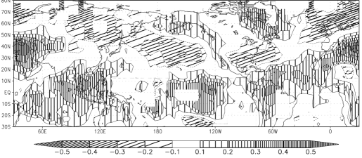
$r_{\mathrm{NINO3},\mathrm{SST}}^{\mathrm{lag}3}$

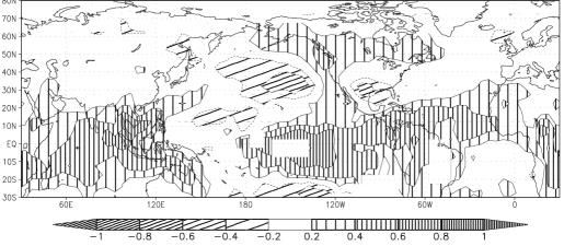
$r_{\mathrm{NINO3},\mathrm{SST}}^{\mathrm{lag}3}\times r_{\mathrm{SST},P(\mathrm{50^{\circ}N})}$

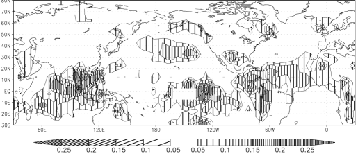
Figure 8: The correlation of spring precipitation around 50^∘N in Europe with the Jones and Parker temperature dataset (top), the lag-3 correlation of this temperature and the NINO3 index (middle) and the product of the these two correlations (bottom). Note the different scales.

		DJF	MAM
		NINO3	NINO3.4	SE Asia	N Pacific	De Bilt	50∘N
DJF	NINO3	1.00	0.80	0.67	0.49	0.35	0.49
MAM	NINO3.4		1.00	0.67	0.50	0.22	0.28
	SE Asia			1.00	0.47	0.36	0.35
	N Pacific				1.00	0.26	0.30
	De Bilt					1.00	0.60
	50∘N						1.00

Table 1: Correlation coefficients between the DJF Kaplan/NCEP NINO3 index; the MAM NINO3.4, SE Asia and North Pacific temperature indices extracted from Parker et al. (1995); and MAM De Bilt and European 50^∘N precipitation.

Figure 9: Lag correlation coefficients of the MAM temperature anomalies in the three possible source regions with the with the NINO3 index, weighted with the correlation coefficients with the Europe 50^∘N precipitation index in spring.

We defined three temperature anomaly indices corresponding to these regions: for the Central Pacific we use the NINO3.4 region, for south-east Asia the box 60^∘E – 120^∘E, 10^∘S – 20^∘N and for the North Pacific dipole the region 160^∘E – 120^∘W, 30^∘N – 60^∘N with a top-left/bottom-right dipole structure. The correlation coefficients between all indices we accumulated are given in Table 1. In figure 9 we plot the lag-correlation coefficients of these indices with the NINO3 index, multiplied by their correlation with the European 50^∘N spring precipitation index. One sees that the shape of the lag structure of the south-east Asian region corresponds closely to the observed signal. Also the signal in pressure (Fig. 7c) is very similar to the lagged NINO3 signal over Europe (Fig. 7b), but the North-African opposite-sign anomaly has disappeared. However, the correlation of the south-east Asia index with rainfall in Europe is only $0.35$, which is lower than the lagged correlation with NINO3 instead of the higher value expected for an intermediate variable. This may partly be due to other mechanisms, such as the direct link from the central Pacific, but also the nature of the measurements plays a role. Temperature differences in the south-east Asia area are small: the MAM variance is only $(0.28\>\mathrm{K})^{2}$, much less than the $(0.88\>\mathrm{K})^{2}$ of the DJF NINO3 index. This increases the effect of noise in the form of measurement errors, irrelevant land points and small-scale weather. On the basis of the time delays of the signal we conclude that south-east Asia is most likely the main source of the influence of ENSO on the weather of Europe, with a smaller direct link from the central Pacific.

The importance of the south-east Asia sea surface temperature for the northern hemisphere circulation is supported by data analyses and modelling studies, see e.g. the review by Trenberth et al. (1998). In spring the most active teleconnection is the North Pacific pattern. This is the top half of Figs 7a,b. The lower halves show an extension across the North Pole into Europe. This extension substantiates arguments using simplified Rossby wave propagation. Unfortunately virtually all modelling studies have been conducted for northern winter conditions, when the observations contain a much weaker teleconnection. Still, indications of the pole-crossing response can be seen in DJF AGCM results (see, e.g., Ferranti et al., 1994). One could speculate that the spring transition to the Asian and Chinese monsoon systems makes the circulation more susceptible to perturbations. Further modelling work is clearly needed in order to elucidate the mechanism behind the teleconnection to Europe.

5 Conclusions

Using more than a century of data a clear influence of ENSO on the weather in Europe has been established: spring precipitation in a belt around 50^∘N from Southern England to the Ukraine tends to increase after an El Niño and decrease after a La Niña. The strength of the correlation is $r=0.49$ for an index of precipitation in this belt, $r=0.40$ for the average of four Dutch stations, and $r=0.35$ for the single station De Bilt. Other European teleconnections are weaker than this. The 3-6 month lag and correlation maps suggest that south-east Asian surface temperatures may act as an intermediate variables for most of the signal.

Acknowledgements

We would like to thank Theo Opsteegh and Robert Mureau for many useful discussions.

References

- Allan et al. (1991) Allan, R.J., Nicholls, N., Jones, P.D., and Butterworth, I.J. 1991. ‘A further extension of the Tahiti-Darwin SOI, early SOI results and Darwin pressure’, J. Climate, 4, 743–749. The series can be found at http://www.cru.uea.ac.uk/cru/data/soi.htm.
- Baker et al. (1995) Baker, C. B., Eischeid, J. K., Karl, T. R., and Diaz, H. F. 1995. ‘The quality control of long-term climatological data using objective data analysis’, in Preprints of AMS Ninth Conference on Applied Climatology Dallas, TX. The data are available from http://www.ncdc.noaa.gov/onlinedata/climatedata/grid.prcp.seasanom.html.
- Basnett and Parker (1997) Basnett, T. A. and Parker, D. E. 1997. ‘Development of the global mean sea level pressure data set GMSLP2’, Climatic Research Technical Note 79 Hadley Centre Meteorological Office, Bracknell, U.K. 16pp plus Appendices. Data are available from http://www.cru.uea.ac.uk/cru/data/pressure.htm.
- Berlage (1966) Berlage, H. P. 1966. The Southern Oscillation and World Weather Number 88 in Mededelingen en verhandelingen. KNMI 152 pp.
- Ferranti et al. (1994) Ferranti, L., Molteni, F., and Palmer, N. 1994. ‘Impact of localized tropical and extratropical SST anomalies in ensembles of seasonal GCM integrations’, Q. J. Meteorol. Soc., 120, 1613–1645.
- Fraedrich (1994) Fraedrich, K. 1994. ‘An ENSO impacty on Europe?’, Tellus, 46A, 541–552.
- Gray (1984) Gray, W. M. 1984. ‘Atlantic seasonal hurricane frequency: Part I: El Niño and 30 mb quasi–biennial oscillation influences’, Mon. Wea. Rev., 112, 1649–1668.
- Halpert and Ropelewski (1992) Halpert, M. S. and Ropelewski, C. F. 1992. ‘Surface temperature patterns associated with the Southern Oscillation’, J. Climate, 5, 577–593.
- Jones (1987) Jones, P. D. 1987. ‘The early twentieth century arctic high — fact or fiction?’, Climate Dynamics, 1, 63–75.
- Jones (1994) Jones, P. D. 1994. ‘Hemispheric surface air temperature variations: a reanalysis and an update to 1993’, J. Climate, 7, 1794–1802.
- Kaplan et al. (1998) Kaplan, A., Cane, M., Kushnir, Y., Clement, A. C., Blumenthal, and Rajagopalan, B. 1998. ‘Analyses of global sea surface temperature 1856–1991’, J. Geophys. Res., 103, 18567–18589. Data are available from http://ingrid.ldgo.columbia.edu.
- Kiladis and Diaz (1989) Kiladis, G. N. and Diaz, H. F. 1989. ‘Global climatic anomalies associated with extremes in the southern oscillation’, J. Climate, 2, 1069–1090.
- Können et al. (1998) Können, G. P., Jones, P. D., Kaltofen, M. H., and Allan, R. J. 1998. ‘Pre-1866 extensions of the Southern Oscillations index using early Indonesian and Tahitian meteorological readings’, J. Climate, 11, 2325–2339.
- Parker et al. (1995) Parker, D. E., Folland, C. K., and Jackson, M. 1995. ‘Marine surface temperature: observed variations and data requirements’, Climatic Change, 31, 559–600.
- Parker et al. (1994) Parker, D. E., Jones, P. D., Bevan, A., and Folland, C. K. 1994. ‘Interdecadal changes of surface temperature since the late 19th century’, J. Geophys. Res., 99, 14373–14399. Data are available from http://www.cru.uea.ac.uk/cru/data/temperat.htm.
- Reynolds and Smith (1994) Reynolds, R. W. and Smith, T. M. 1994. ‘Improved global sea surface analyses using optimum interpolation’, J. Clim., 7, 929–948. Nino indices are available from the Climate Prediction Center at http://nic.fb4.noaa.gov/data/cddb/altindex.html.
- Trenberth et al. (1998) Trenberth, K. E., Branstator, G. W., Karoly, D., Kumar, A., Lau, N.-C., and Ropelewski, C. 1998. ‘Progress during TOGA in understanding and modeling global teleconnections associated with tropical sea surface temperatures’, J. Geophys. Res., 103, 14291–14324.
- van Loon and Madden (1981) van Loon, H. and Madden, R. A. 1981. ‘The Southern Oscillation, Part I. Global associations with pressure and temperature in northern winter’, Mon. Wea. Rev., 109, 1150–1162.
- Wilby (1993) Wilby, R. 1993. ‘Evidence of ENSO in the synoptic climate of the British Isles since 1880’, Weather, 48, 234–239.