Application of time-dependent density functional theory to optical activity

Abstract

As part of a general study of the time-dependent local density approximation (TDLDA), we here report calculations of optical activity of chiral molecules. The theory automatically satisfies sum rules and the Kramers-Kronig relation between circular dichroism and optical rotatory power. We find that the theory describes the measured circular dichroism of the lowest states in methyloxirane with an accuracy of about a factor of two. In the chiral fullerene C₇₆ the TDLDA provides a consistent description of the optical absorption spectrum, the circular dichroism spectrum, and the optical rotatory power, except for an overall shift of the theoretical spectrum.

I Introduction

The time-dependent local density approximation (TDLDA) as well as the time-dependent Hartree-Fock theory has been applied to the optical absorption of atomic and molecular systems with considerable success [1-14]. Here we want to see how well the TDLDA method does on a more subtle aspect of the optical response, the optical activity of chiral molecules. Calculation of circular dichroism and especially optical rotatory power is more challenging because the operators that must be evaluated are more sensitive to the approximations on the wave function than the electric dipole in the usual form $e\vec{r}$. Nevertheless, we anticipate that TDLDA may be a useful theory because the operators are still of the form of single-electron operators. The TDLDA is derived by optimizing a wave function constructed from (time-dependent) single-particle wave functions, so its domain of validity is the one-particle observables.

In our implementation of TDLDA [8], we represent the electron wave function on a uniform spatial grid. The real-time evolution of the wave function is directly calculated and the response functions are calculated by the time-frequency Fourier transformation. The method respects sum rules and the Kramers-Kronig relation between the circular dichroism and optical rotatory power. Since the grid representation is bias-free with respect to electromagnetic gauge, it is not subject to the gauge difficulties encountered when the space of the wave function is constructed from an atomic orbital representation.

Optical activity has been a challenging problem for computational chemistry, but there has been considerable progress in recent years. For example, Carnell et al. [15] present a good description of the circular dichroism of excited states of R-methyloxirane using a standard Gaussian representation of the wave function. The optical rotatory power is a much more difficult observable, since the whole spectrum contributes. Only very recently have $ab~{}initio$ calculations been reported for this property[16, 17].

After presenting our calculational method, we report our exploratory study on optical activities of two chiral molecules: R-methyloxirane, a simple 10-atom molecule with known chiroptical properties up to the first few excited states[15, 18, 19], and C₇₆, a fullerene with very large optical rotatory power and significant circular dichroism in the visible and UV[20].

II Formalism

A Some definitions

Polarization of chiral molecule in applied electromagnetic field is expressed using two coefficients $\alpha$ and $\beta$ as [21]

$$\vec{p}=\alpha\vec{E}-\frac{\beta}{c}\frac{\partial\vec{H}}{\partial t}.$$ (1)

Here $\alpha$ is the usual polarizability and is given microscopically as

$$\alpha(E)=e^{2}\sum_{n}\left(\frac{1}{E_{n0}-E-i\delta}+\frac{1}{E_{n0}+E+i\delta}\right)\frac{1}{3}\langle\Phi_{0}|\sum_{i}\vec{r}_{i}|\Phi_{n}\rangle^{2},$$ (2)

where $\Phi_{n}$ and $E_{n}$ are the eigenvector and eigenvalue of the $n$-th eigenstate of the many-body Hamiltonian $H$, $H\Phi_{n}=E_{n}\Phi_{n}$, and $E_{n0}=E_{n}-E_{0}$. The $\delta$ is an infinitesimal positive quantity. Employing the oscillator strength

$$f_{n}=\frac{2mE_{n}}{\hbar^{2}}\frac{1}{3}\langle\Phi_{0}|\sum_{i}\vec{r}_{i}|\Phi_{n}\rangle^{2},$$ (3)

we define the optical absorption strength whose integral is normalized to the active electron number,

$$S(E)=\sum_{n}\delta(E-E_{n})f_{n}.$$ (4)

It is related to the imaginary part of the polarizability,

$$S(E)=\frac{2mE}{\hbar^{2}e^{2}}\frac{{\rm Im}\alpha(E)}{\pi}.$$ (5)

The basic quantity which characterizes the chiroptical transition is the rotational strength defined by [22]

$$R_{n}=-\frac{e^{2}\hbar}{2mc}\langle\Phi_{0}|\sum_{i}\vec{r}_{i}|\Phi_{n}\rangle\cdot\langle\Phi_{n}|\sum_{i}\vec{r}\times\vec{\nabla}|\Phi_{0}\rangle.$$ (6)

We define the complex rotational strength function,

$${\cal R}(E)=\sum_{n}\left(\frac{1}{E_{n0}-E-i\delta}-\frac{1}{E_{n0}+E+i\delta}\right)R_{n}.$$ (7)

The beta function in eq.(1) is related to ${\cal R}(E)$ by $\beta(E)=\frac{\hbar c}{3E}{\cal R}(E)$. We will also use the rotational strength function $R(E)$ defined by

$$R(E)=\sum_{n}\delta(E-E_{n})R_{n}=\frac{{\rm Im}{\cal R}(E)}{\pi}.$$ (8)

As is seen below, the optical rotatory power is proportional to the real part of $\beta(E)$, and the circular dichroism to $R(E)$. They are related to each other by the Moscowitz’s generalized Kramers-Kronig relation [23].

The difference of complex indices of refraction for left and right circularly polarized light is proportional to ${\cal R}$ in dilute media; the relation is

$$n_{L}-n_{R}={8\pi N_{1}\over 3}{\cal R}(E),$$ (9)

where $N_{1}$ is the number of molecules per unit volume. For comparison with experiment, the common measure of circular dichroism is the decadic extinction coefficient, given by

$$\Delta\epsilon={4\pi\over\lambda_{cm}C\log_{e}10}{\rm Im}(n_{L}-n_{R}),$$ (10)

where $C$ is the concentration of molecules in moles/liter and the subscript on the wavelength $\lambda$ is a reminder to express it in centimeters. The optical rotatory power is conventionally reported as

$$[\alpha]=180^{\circ}{10\over C_{gm}\lambda}{\rm Re}(n_{L}-n_{R}),$$ (11)

where $C_{gm}$ is the concentration of molecules in gm/cm³.

B Real-time TDLDA

We first rewrite the above strength functions as time integrations. We employ the time dependent wave function $\Psi(t)=\exp[-iHt/\hbar]\Psi(0)$ with the initial wave function at $t=0$ given by $\Psi(0)=\exp[ik\sum_{i}z_{i}]\Phi_{0}$, where $k$ is a small wave number. In the linear response, the time-dependent polarizability is proportional to the dipole matrix element, $z(t)=\langle\Psi(t)|\sum_{i}z_{i}|\Psi(t)\rangle$. The frequency dependent polarizability in $z$ direction is then obtained as the time-frequency Fourier transformation of $z(t)$,

$$\alpha_{z}(E)=\frac{e^{2}}{k}\int_{0}^{\infty}\frac{dt}{\hbar}e^{i(E+i\delta)t/\hbar}z(t).$$ (12)

The polarizability $\alpha(E)$ is given by the orientational average, $\alpha=(\alpha_{x}+\alpha_{y}+\alpha_{z})/3$.

Similarly, we denote the angular momentum expectation value as $L_{z}(t)=\langle\Psi(t)|-i(\vec{r}\times\nabla)_{z}|\Psi(t)\rangle$. To linear order in $k$, we may express it as

$$L_{z}(t)=-2k\sum_{n}\cos\left(\frac{E_{n0}t}{\hbar}\right)\langle\Phi_{0}|\sum_{i}z_{i}|\Phi_{n}\rangle\langle\Phi_{n}|\sum(\vec{r}_{i}\times\vec{\nabla}_{i})_{z}|\Phi_{0}\rangle.$$ (13)

The complex rotatory strength function ${\cal R}(E)$ is expressed as,

$${\cal R}_{z}(E) = \frac{e^{2}\hbar}{2mc}\frac{i}{k}\int_{0}^{\infty}\frac{dt}{\hbar}e^{(E+i\delta)t/\hbar}L_{z}(t)$$ (14)

$$= \frac{e^{2}\hbar}{2mc}\sum_{n}\left(\frac{1}{E_{n0}-E-i\delta}-\frac{1}{E_{n0}+E+i\delta}\right)\langle\Phi_{0}|\sum_{i}z_{i}|\Phi_{n}\rangle\langle\Phi_{n}|\sum_{i}(\vec{r}\times\vec{\nabla})_{z}|\Phi_{0}\rangle.$$ (15)

${\cal R}(E)$ of eq.(7) is the sum over three directions, ${\cal R}={\cal R}_{x}+{\cal R}_{y}+{\cal R}_{z}$.

In the time-dependent local density approximation, the time-dependent wave function $\Psi(t)$ is approximated by a single Slater determinant. We prepare the initial single electron orbitals as $\psi_{i}(0)=\exp[ikz]\phi_{i}$ where $\phi_{i}$ is the static Kohn-Sham orbitals in the ground state. The $\psi_{i}(t)$ follows the time-dependent Kohn-Sham equation,

$$i\hbar\frac{\partial}{\partial t}\psi_{i}(t)=\left\{-\frac{\hbar^{2}}{2m}\nabla^{2}+\sum_{a}V_{ion}(\vec{r}-\vec{R}_{a})+e^{2}\int d\vec{r}^{\prime}\frac{\rho(\vec{r}^{\prime},t)}{|\vec{r}-\vec{r}^{\prime}|}+\mu_{xc}(\rho(\vec{r},t))\right\}\psi_{i}(t),$$ (16)

where $V_{ion}$ is the electron-ion potential and $\mu_{xc}$ is the exchange-correlation potential. The time-dependent density is given by $\rho(\vec{r},t)=\sum_{i}|\psi(\vec{r},t)|^{2}$. The time-dependent dipole moment may be evaluated as $z(t)=\sum_{i}\langle\psi_{i}|z|\psi_{i}\rangle$ and the similar expression for $L_{z}(t)$. The strength functions are then evaluated with eqs.(12) and (14).

C Sum rules

According to the TRK sum rule, the integral of $S(E)$ is equal to the number of active electrons $N$. This sum rule is respected by the TDLDA. It also appears in the short time behavior of $z(t)$ as

$$z(t)=N\frac{\hbar k}{m}t~{}~{}~{}~{}~{}~{}~{}(t~{}small)$$ (17)

For the rotational strength, we define energy-weighted sums as

$$R^{(n)}=\int_{0}^{\infty}dEE^{n}R(E).$$ (18)

It is known that $R^{(n)}$ for $n\leq 4$ vanishes identically in the exact dynamics [22, 24, 25, 26]. The vanishing of $R^{(0)}$ in the time-dependent Hartree-Fock theory was first noticed in [27]. The short time behavior of $L(t)=L_{x}(t)+L_{y}(t)+L_{z}(t)$ is related to $R^{(n)}$ as

$$\frac{e^{2}\hbar}{2mc}L(t)=2k\left\{R^{(0)}-\frac{R^{(2)}}{2!}\left(\frac{t}{\hbar}\right)^{2}+\frac{R^{(4)}}{4!}\left(\frac{t}{\hbar}\right)^{4}-\frac{R^{(6)}}{6!}\left(\frac{t}{\hbar}\right)^{6}+...\right\}$$ (19)

Here we note that $L(t)$ is an even function of $t$ as seen in eq.(13). Since $R^{(n)}=0$ for $n\leq 4$, we see that $L(t)$ behaves as $t^{6}$ for small time. $L_{i}(t)(i=x,y,z)$ behave as $t^{2}$ at small $t$ and the cancelation up to $t^{4}$ order occurs after summing up three directions. In the TDLDA dynamics, we confirmed that at least $t^{0}$ and $t^{2}$ coefficients of $L(t)$, namely $R^{(0)}$ and $R^{(2)}$, vanish identically.

D Numerical detail

The TDLDA uses the same Kohn-Sham Hamiltonian as is used in ordinary static LDA calculations. As is common in condensed matter theory, we use pseudopotentials that include the effects of $K$-shell electrons rather than include these electrons explicitly. The pseudopotentials are calculated by the prescriptions of ref. [28] and [29]. We employ the simple exchange-correlation term proposed in ref. [30, 31]. There are improved terms now in use[33, 32], but it was not deemed important for our application.

There are many numerical methods to solve the equations of TDLDA. Ours uses a Cartesian coordinate space mesh to represent the electron wave functions, and the time evolution is calculated directly [8, 9, 34]. There are only four important numerical parameters in this approach: the mesh spacing, the number of mesh points, the time step in the time integration algorithm, and the total length of time that is integrated. We have previously found that the carbon molecules can be well treated using a mesh spacing of 0.3 Å[9, 34]. We find 0.25 Å is necessary for methyloxirane to represent accurately the orbitals around oxygen. We take the spatial volume to be a sphere of radius 8 Å both for methyloxirane and C₇₆ presented below. The total number of mesh points, defining the size of the vector space, is about $4\pi R^{3}/(3\Delta x^{3})\sim 80,000(140,000)$ for mesh size of 0.3 Å(0.25 Å).

The algorithm for the time evolution is quite stable as long as the time step $\Delta t$ satisfies $\Delta t<\hbar/|H|$, where $|H|$ is the maximum eigenvalue of the Hamiltonian. This is mainly dependent on the mesh size. For $\Delta x=0.3$ Å, we find that $\Delta t=0.002\hbar$/eV is adequate. We integrate the equation of motion for a length of time $T=60\hbar$/eV for C₇₆ ($50\hbar$/eV for methyloxirane). Then individual states can be resolved if their energy separation satisfies $\Delta E>2\pi\hbar/T\sim 0.1$eV.

Our numerical implementation, grid representation of the wave function and the time-frequency Fourier transformation for the response calculation, has several advantages over the usual approach using basis functions centered at the ions. They include:
(1) The full spectrum of wide energy region may be calculated at once and it respects sum rules. The non-locality of the pseudopotential may cause violation of the sum rule, but the effect is small in the present systems.
(2)Since the circular dichroism $R(E)$ and the optical rotatory power, real part of $\beta(E)$, are calculated as Fourier transformation of single function $L(t)$, the Kramers-Kronig relation is automatically satisfied.
(3)The gauge independence of the results is satisfied to high accuracy. Employing the commutation relation $[H,\sum_{i}\vec{r}_{i}]=-\frac{\hbar^{2}}{m}\sum_{i}\vec{\nabla}_{i}$, there is alternative expressions for optical transitions with gradient operator instead of coordinate. For the rotational strength, for example,

$$R_{n}=-\frac{e^{2}\hbar^{3}}{2m^{2}cE_{n0}}\langle\Phi_{0}|\sum_{i}\vec{\nabla}_{i}|\Phi_{n}\rangle\cdot\langle\Phi_{n}|\sum_{i}{\vec{r}}_{i}\times{\vec{\nabla}}_{i}|\Phi_{0}\rangle,$$ (20)

The strength function with this expression may be calculable with initial wave function $\psi_{i}(0)=\exp[id\nabla_{z}]\phi_{i}$ with small displacement parameter $d$. Since the grid representation of wave function does not have any preference on the gauge condition, our method gives almost identical results for the coordinate and gradient expressions of dipole matrix elements.

III R-methyloxirane

The geometry of R-methyloxirane is shown in Fig. 1. We use the same nuclear distances as in ref. [15]. We show in Fig. 2 the results of the static calculation for the orbital energies. We find a LUMO 6.0 eV above the HOMO, and a triplet of unoccupied states 0.5 eV higher. In our calculation the lowest unoccupied orbitals have an diffuse, Rydberg-like character, $s$-wave for the lower and $p$-wave for the upper, as in previous calculations[15, 35]. The HOMO is localized in the vicinity of the oxygen atom, and the measured absorption strength seen at 7.1 and 7.7 eV is attributed to the excitation of a HOMO electron to the diffuse states. In the TDLDA, the excitation energy comes out close to the orbital difference energies, except for strongly collective states. Indeed we find in the TDLDA calculation that the excitations are within 0.1 eV of the HOMO-LUMO energy and the energy difference for the next state above the LUMO. This is one eV less than the experimental values. It is known that the LDA energy functional that we use is subject to overbind excitations close to the ionization threshold. There are improved energy functions that rectify this problem[36], but for this work we judged the error not important.

The next property we examine is related to the electric dipole matrix element, namely the oscillator strength $f$ associated with the transition. The optical absorption strength is shown in Fig. 3. The total strength up to 100 eV excitation is f=22.4, which is 93% of the sum rule for the 24 active electrons. Notice the lowest two peaks, centered at 6.0 and 6.5 eV. These are the states we are interested in. Their oscillator strengths are given in Table I. We see that the states are both weak, less than a tenth of a unit. The effect of the time-dependent treatment is to lower the strengths by 30-50%. This is the well-known screening effect associated with virtual transitions of more deeply bound orbitals. We find that the computed transition strengths are within a factor of two of the measured ones. Typically, the TDLDA does somewhat better than this, but most of the experience has been with transitions carrying at least a tenth of a unit of oscillator strength. The original theoretical calculation gave very poor transition strengths[18], off by more than an order of magnitude. Unfortunately, the more recent study[15] did not include theoretical transition strengths.

We numerically confirmed that our method gives almost identical results with coordinate and gradient expressions of dipole matrix elements, as we noticed in the previous section. However, exceptionally, the oscillator strength of the very weak features discussed above suffer substantial dependence on the expression. With gradient formula for the transition matrix elements, strengths of both first and second transitions are larger by about factor two than the coordinate expression. Since the gradient formula emphasizes high-momentum components more heavily, we think the results with coordinate matrix elements may be more reliable for low transitions, and we quote them in Table I.

We now turn to the chiroptical response. Fig. 4 shows the short-time behavior of $L_{x}(t)$ and the sum of the three Cartesian components $L(t)=\sum_{i}L_{i}(t)$. An initial perturbation of $k=0.001$ Å^-1 is employed. To within numerical precision, $L_{x}(t)$ (solid line) grows with time as $t^{2}$, as discussed below eq.(18). The same is true for the other two components, $L_{y}$ and $L_{z}$. This shows that the numerical algorithm respects the first sum rule. The combined response, $L(t)$ (dashed lines) shows an extreme cancelation at short times, as required by the additional sum rules. However our numerical accuracy does not allow us to determine the order of the power behavior. The evolution of $L(t)$ for larger times is shown in Fig. 5. Physically, the TDLDA breaks down at long times because of coupling to other degrees of freedom. A typical width associates with such couplings is of the order of a tenth of an eV, implying that the responses damp out on a time scale of $T\approx 10\hbar$/eV. We note that the TDLDA algorithm itself is very stable, and allows us to integrate to much larger times and obtain very sharp theoretical spectra.

We next show the Fourier transform of the chiroptical response. The circular dichroism spectrum calculated with eq. (14) is shown in Fig. 6. Here we have integrated $L$ to $T=50\hbar$/eV, including a filter function in the integration to smooth the peaks. One can see that the $s$- and the $p$-transitions are clearly resolved, although the three $p$-transitions are not resolved from each other (as is the experimental case). The $s$-transition has a negative circular dichroism and the $p$-transition a positive one. Integrating over the peaks, the strengths of the two peaks are -0.0014 and +0.0014 ų-eV, respectively. The strengths are commonly quoted in cgs units; the conversion factor is 1 eV-ų = 1.609 $\times 10^{-36}$ erg-cm³. The values in cgs units are given in Table I, compared to experiment and previous calculations. We find the signs are correctly given, but the values are somewhat too high, by a factor of 2 or 3. The calculation of ref.[15] gave a result within the experimental range for the $p$-multiplet but too small (by a factor of 2) for the $s$-transition. Thus we find that the TDLDA has a somewhat poorer accuracy in this case.

Next we consider the optical rotatory power. It could be calculated as the real part of the Fourier transformation eq.(14). In practice, however, we found the calculation employing Kramers-Kronig relation to the rotational strength function,

$${\rm Re}\beta(E)=\frac{2}{3}\hbar c\int_{0}^{\infty}dE^{\prime}\frac{R(E^{\prime})}{{E^{\prime}}^{2}-E^{2}},$$ (21)

gives more accurate result especially at the energy below the lowest transition. The measurement is available at sodium D-line, 2.1 eV, $[\alpha]_{D}=+14.65^{\circ}$ [35] which gives $\beta=+0.0017$ Å⁴. The calculated value at low energy is very sensitive to the number of states included in the sum. Fig.6 shows the calculated value as a function of a cutoff energy, upper bound in the integration in eq.(20). The value taking only the contribution of the lowest transition is -0.06. Including more states produces values that fluctuate in sign and magnitude within that range. Including all states below 100 eV gives a cancelation by a factor of 60 to yield a value $\beta=-0.001$ Å⁴. This has the opposite sign but the same order of magnitude as the measured $\beta$. Clearly, to get high relative accuracy with such a strong cancelation is more demanding than our TDLDA can provide.

IV C₇₆

Remarkably, it is possible to separate the chiral partners of the double-helical fullerene C₇₆ using stereospecific chemistry[20]. The molecule shows a huge optical rotatory power, $[\alpha]_{D}=-4000^{\circ}$, and a complex circular dichroism spectrum between 2 and 4 eV excitation [20]. There has been reported only semi-empirical quantum chemistry calculation for the optical activity of this molecule [37].

We first remark on the geometry of the molecule, which has a chiral $D_{2}$ symmetry[38]. The accepted geometry is depicted in ref.[20]; it may be understood as follows. We start with C₆₀, in which all carbons on pentagons. Group the pentagons into triangles and divide the fullerene in half keeping two adjacent triangles of pentagons intact in each half. The “peel” of six pentagons already has a chiral geometry dependent on the relative orientation of its two triangles of pentagons. The C₇₆ is constructed by adding 16 carbon atoms between the split halves of the C₆₀. The added carbon atoms lie entirely on hexagons which form a complete band around the fullerene. The inserted band has the geometry of an (8,2) chiral buckytube. The result is then the chiral C₇₆. Our calculations are performed on a right-handed C₇₆, in the sense that the band of hexagons corresponds to a right-handed buckytube. This is the same convention as used in ref. [38], their Fig. 3d.

The C₇₆ has 152 occupied spatial orbitals. We show the orbitals near the Fermi level in Fig. 8. The HOMO-LUMO gap is only 0.9 eV, and there are many transition in the optical region. In Fig. 9 we show the optical absorption strength function for the range 0-50 eV. Smoothing is made with the width of 0.2 eV in the Fourier transformation. A concentration of strength is apparent at 6 eV excitation; there is a similar peak in graphite and C₆₀  which is associated with $\pi-\pi^{*}$ transitions. The strong, broad peak centered near 20 eV is associated with $\sigma-\sigma^{*}$ transitions and is also present in C₆₀  [34]. The feature at 13 eV is not present in C₆₀ , however. In the next figure, Fig. 10, we show a magnified view of the absorption at low energy. We also compare the TDLDA strength with the single-electron strength, smoothed also by convolution with a Breit-Wigner function of width $\Gamma=0.2$ eV. The TDLDA has a strong influence on the strength distribution, decreasing the total strength in the low energy region and concentrating in the 6 eV peak. The experimental absorption strength [38] (with arbitrary normalization) is shown as the dashed line. It agrees with the TDLDA quite well.

We next examine the circular dichroism spectrum. Fig. 11 shows the rotatory strength function between 0 and 50 eV. Like the case of methyloxirane, it is irregular without any large scale structures. Its integral is zero to an accuracy of 0.001 eV-ų. The low energy region is shown in Fig. 12. Here one sees qualitative similarities between theory and experiment [20]. The theoretical sharp negative peak at 1.8 eV corresponds to an experimental peak at 2.2 eV. Shifting the higher spectra by that amount (0.6 eV), one sees a correspondence between the next positive and negative excursions. We note that a similar shift in the excitation energy was also seen in the optical absorption of C₆₀  between the measurement and the TDLDA calculation [34].

Our theoretical optical rotatory power is plotted in Fig. 13. The situation here is different from the methyloxirane, in that rotatory power is large in a region where there are allowed transitions. The measured optical rotatory power, $[\alpha]_{D}=-4000^{\circ}$ at 2.1 eV [20] corresponding to $\beta=-7.3$ Å⁴, is shown as the star. It does not agree with theory, but we should remember that the spectrum needs to be shifted by 0.6 eV to reproduce the circular dichroism. Adjusting the theoretical spectrum upward by that amount, we find that it is consistent in sign and order of magnitude with the measurement. Since the optical rotatory power in the region of allowed transitions changes rapidly as excitation energy, a measurement of the energy dependence would be very desirable, and would allow a more rigorous comparison with the theory.

V Concluding remarks

We have presented an application of the time-dependent local density approximation to the optical activities of chiral molecules. Our method is based on the uniform grid representation of the wave function, real-time solution of the time-dependent Kohn-Sham equation, and the time-frequency Fourier transformation to obtain the response functions. In this way we can calculate the optical absorption, circular dichroism, and the optical rotatory power over a wide energy region, respecting sum rules and Kramers-Kronig relation.

We applied our method to two molecules, methyloxirane and C₇₆. For lowest two transitions of methyloxirane, the TDLDA reproduces the absorption and rotational strength in the accuracy within factor two. The qualitative feature of the circular dichroism spectrum of C₇₆ is also reproduced rather well. However, the optical rotatory power is found to be a very sensitive function with strong cancelation. Even though we obtained rotational strength of full spectral region, it is still difficult to make quantitative prediction of optical rotatory power at low energies in our present approach.

VI Acknowledgment

We thank S. Saito for providing us with coordinates of C₇₆. We also thank him, S. Berry, and B. Kahr for discussions. This work is supported in part by the Department of Energy under Grant DE-FG-06-90ER40561, and by the Grant-in-Aid for Scientific Research from the Ministry of Education, Science and Culture (Japan), No. 09740236. Numerical calculations were performed on the FACOM VPP-500 supercomputer in the institute for Solid State Physics, University of Tokyo, and on the NEC sx4 supercomputer in the research center for nuclear physics (RCNP), Osaka University.

TABLE I.: Transitions in R-methyloxirane

Level		TDLDA	LDA(Free)	Other theory		Experiment
				ref. [15]	ref. [18]	ref. [15]	ref. [18]
1	$E$ (eV)	6.0	5.97	6.25(7.12)	6.40	7.07	7.12
	$f$	0.012	0.021		0.0004∗		0.025
	$R$ ($\times 10^{40}$ cgs)	-23.0	-10.4	-6.43	-2.66∗,∗∗	-12.56	-11.8∗∗
2-4	$\overline{E}$ (eV)	6.5	6.55	6.95	7.3	7.70	7.75
	$\Sigma f$	0.044	0.069		0.0012∗		0.062
	$\Sigma R$ ($\times 10^{40}$ cgs)	23.	29.9	7.93	2.24∗,∗∗	6.98	10.8∗∗

^∗ Calculation with coordinate expression of dipole moment.
^∗∗ Negative of value for S-methyloxirane.

Figure Captions

Fig. 1. View of R-methyloxirane with hydrogen on the chiral carbon in the back (and not seen). The chirality is R because the three other bonds are arrange clockwise in the sequence O, CH₃, CH₂.

Fig. 2 Static LDA orbitals in methyloxirane.

Fig. 3 Optical absorption strength of methyloxirane in the energy region 0-50 eV.

Fig. 4 Short-time chiroptical response of R-methyloxirane. Solid line is $L_{x}(t)$, dashed line is $\sum_{i}L_{i}(t)$.

Fig. 5 Chiroptical response of R-methyloxirane $L(t)$ for longer times.

Fig. 6 $R$ in R-methyloxirane in the interval 0-20 eV.

Fig. 7 Optical rotatory power Re$\beta$ at $E=2.1$ eV as a function of cutoff energy $E_{max}$ in the integration of eq. (20).

Fig. 8 Static LDA orbitals in C₇₆ near the Fermi level.

Fig. 9 Optical absorption spectrum of C₇₆ in the range 0-50 eV.

Fig. 10  Optical absorption spectrum of C₇₆ in the range 0-8 eV. Dotted line is the single-electron strength, solid line the TDLDA, and dashed line experiment[38].

Fig. 11  Circular dichroism spectrum of C₇₆.

Fig. 12  Circular dichroism spectrum of C₇₆ comparing theory (solid line) and experiment (dashed line). The experimental data is from ref. [20] and is with arbitary normalization.

Fig. 13  Optical rotatory power of C₇₆, given as Re$\beta$ in unit of Å⁴. The cross is the measured value from $[\alpha]_{D}$.

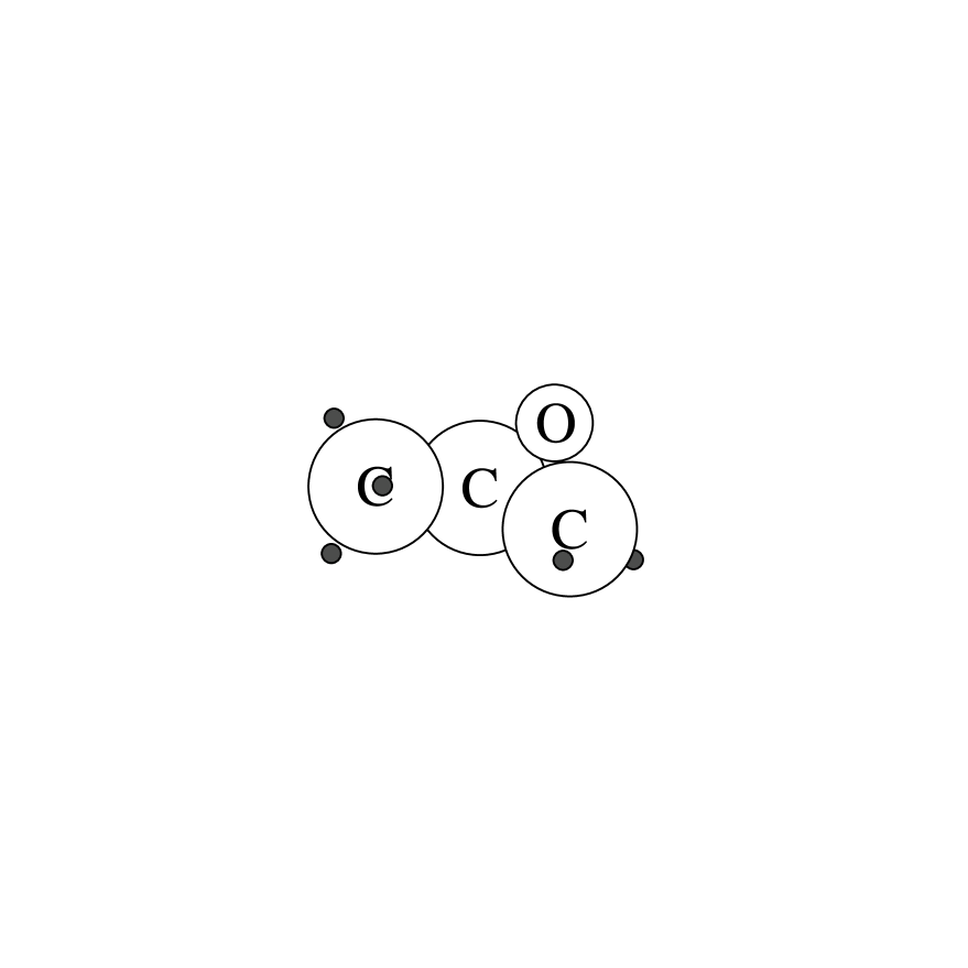
FIG. 1.: View of R-methyloxirane with hydrogen on the chiral carbon in the back (and not seen). The chirality is R because the three other bonds are arrange clockwise in the sequence O, CH₂O,CH₃.

FIG. 2.: Static LDA orbitals in methyloxirane.

FIG. 3.: Optical absorption strength of methyloxirane in the energy region 0-50 eV.

FIG. 4.: Short-time chiroptical response of R-methyloxirane. Solid line is $L_{x}(t)$, dashed line is $\sum_{i}L_{i}(t)$, in units of Å.

FIG. 5.: Chiroptical response of R-methyloxirane $L(t)$ for longer times.

FIG. 6.: $R$ in R-methyloxirane in the interval 0-20 eV.

FIG. 7.: Optical rotatory power Re$\beta$ at $E=2.1$ eV as a function of cutoff energy $E_{max}$ in the integration of eq. (20).

FIG. 8.: Static LDA orbitals in C₇₆ near the Fermi level.

FIG. 9.: Optical absorption spectrum of C₇₆ in the range 0-50 eV.

FIG. 10.: Optical absorption spectrum of C₇₆ in the range 0-8 eV. Dotted line is the single-electron strength, solid line the TDLDA, and dashed line experiment[38].

FIG. 11.: Circular dichroism spectrum of C₇₆.

FIG. 12.: Circular dichroism spectrum of C₇₆ comparing theory (solid line) and experiment (dashed line). The experimental data is from ref. [20] and is with arbitary normalization.

FIG. 13.: Fig. 13  Optical rotatory power of C₇₆, given as Re$\beta$ in unit of Å⁴. The cross is the measured value from $[\alpha]_{D}$.

REFERENCES

- [1] A. Zangwill and P. Soven, Phys. Rev. A21 1561(1980).
- [2] Z.H. Levine and P. Soven, Phys. Rev. A29 625 (1984).
- [3] H. Zhong, Z.H. Levine and J.W. Wilkins, Phys. Rev. A43 462 (1991).
- [4] F. Alasia et al., J. Phys. B27 L643 (1994).
- [5] M. Stener, P. Decleva and A. Lisini, J. Phys. B28 4973 (1995).
- [6] C. Jamorski, et al, J. Chem. Phys. 104 5134 (1996).
- [7] A. Rubio, et al., Phys. Rev. Lett. 77 247 (1996).
- [8] K. Yabana and G.F. Bertsch, Phys. Rev. B54 4484 (1996).
- [9] K. Yabana and G.F. Bertsch, Z. Phys. D42 219 (1997).
- [10] C. Ullrich and E. Gross, Comments At. Mol. Phys. 33 211 (1997).
- [11] M. Feyereisen, et al., J. Chem. Phys. 96 2978 (1992).
- [12] H. Koch, et al., Chem. Phys. 172 12 (1993).
- [13] Y. Luo, et al., J. Phys. Chem. 98 7782 (1994).
- [14] Y. Luo, et al., Phys. Rev. B51 14949 (1995).
- [15] M. Carnell, et al., Chem. Phys. Lett. 180 477 (1991).
- [16] P.L. Polavarapu and D.K. Chakraborty, J. Am. Chem. Soc. 120 6160 (1998).
- [17] M. Pericou-Cayere, et al., Chem. Phys. 226 297 (1998).
- [18] D. Cohen, et al., J. Am. Chem. Soc. 105 1738 (1983).
- [19] A. Breest, et al., Mol. Phys. 82 539 (1994).
- [20] J.M. Hawkins and A. Meyer, Science 260 1918 (1993)
- [21] E.U. Condon, Rev. Mod. Phys. 9 432 (1937).
- [22] A.E. Hansen and T.D. Bouman, Adv. Chem. Phys. 44 545 (1980).
- [23] A. Moscowitz, Adv. Chem. Phys. 4 67 (1962).
- [24] A.E. Hansen, Mol. Phys. 33 483 (1977).
- [25] D. Caldwell, Mol. Phys. 33 495 (1977).
- [26] I.B. Khriplovich and M.E. Pospelov, Phys. Lett. A171 349 (1992).
- [27] R.A. Harris, J. Chem. Phys. 50 3947 (1969).
- [28] N. Troullier, J.L. Martins, Phys. Rev. B43 1993 (1991).
- [29] L. Kleinman and D. Bylander, Phys. Rev. Lett. 48 1425 (1982).
- [30] D. Ceperley and B. Alder, Phys. Rev. Lett. 45 566 (1980).
- [31] J. Perdew and A. Zunger, Phys. Rev. B23 5048 (1981).
- [32] L. van Leeuwen and E. J. Baerends, Phys. Rev. A49 2421 (1994).
- [33] J.P. Perdew, K. Burke, and M. Ernzerhof, Phys. Rev. Lett. 77 3865 (1996).
- [34] K. Yabana and G.F. Bertsch, preprint physics/9808015, submitted to J. Chem. Phys.
- [35] A. Rank, J. Am. Chem. Soc. 103 1023 (1981).
- [36] M.E. Casida, C. Jamorski, K. Casida, and D.R. Salahub, J. Chem. Phys. 108 4439 (1998).
- [37] G. Orlandi, et al., Chem. Phys. Lett. 224 113 (1994).
- [38] R. Ettl, I. Chao, F. Diederich, and R.L. Whetten, Nature 353 149 (1991).