Markov analysis of stochastic resonance in a periodically driven integrate-fire neuron

Abstract

We model the dynamics of the leaky integrate-fire neuron under periodic stimulation as a Markov process with respect to the stimulus phase. This avoids the unrealistic assumption of a stimulus reset after each spike made in earlier work and thus solves the long-standing reset problem. The neuron exhibits stochastic resonance, both with respect to input noise intensity and stimulus frequency. The latter resonance arises by matching the stimulus frequency to the refractory time of the neuron. The Markov approach can be generalized to other periodically driven stochastic processes containing a reset mechanism.

I Introduction

Periodically modulated stochastic processes have been studied intensely over the last two decades under the paradigm of stochastic resonance: the transduction of signals is optimal in the presence of a particular amount of noise. First suggested to explain the periodicity of ice-ages [1], stochastic resonance has since been demonstrated in a wide range of experiments and the underlying mechanisms are well understood. A recent review of the field is given in [2].

The concept of stochastic resonance has met with particular attention in the neurosciences [3, 4, 5, 6, 7]. The brain achieves an enormous signal processing performance in the presence of noise from a wide range of sources, ranging from stochastic membrane channel openings on a molecular level, via highly irregular firing patterns of individual neurons to distracting stimuli in perception. The improvement of signal transduction on all of these levels has now been demonstrated experimentally [8, 9, 10]. Recently, the first direct evidence for the behavioral relevance of stochastic resonance has been reported [11], underlining the importance of stochastic resonance in neurobiology.

In short, neurons are threshold devices that receive an input $I(t)$ which charges the membrane of the neuron like a leaky capacitor. When the potential $v(t)$ across the membrane reaches a threshold $\Theta$, a spike is fired: the membrane potential makes a brief but strong excursion (duration $\approx 2$ms, amplitude $\approx 100$mV). This spike is transmitted as output to other neurons. After the spike, the membrane potential is reset to a resting value $v_{0}$, some $30$mV below the threshold [12]. As the shape of the spikes is stereotypical, information is only conveyed by the spike times.

This has led to the leaky integrate-fire model of neuronal dynamics [13]. In between two spikes, the membrane potential is governed by

$$\tau_{m}\dot{v}(t)=-v(t)+I(t)+\zeta(t)\>.$$ (1)

Here, $\tau_{m}$ is the time-constant of the membrane, which represents the internal time-scale of the neuron and $\zeta(t)$ is an as yet undefined noise process, comprising, e.g., stochastic membrane potential fluctuations and irregular input to the neuron from sources uncorrelated to $I(t)$. As the potential reaches the threshold, a spike is recorded and the potential is reset to $v(t)=v_{0}$ instantaneously.

For Gaussian white noise $\zeta(t)$ the evolution of the membrane potential $v(t)$ from reset potential to threshold is equivalent to an Ornstein–Uhlenbeck process with drift $I(t)$ and an absorbing boundary at $v=\Theta$. The output of the neuron is modeled as a sequence of delta pulses $f(t)=\sum_{k}\delta(t-t_{k})$ at the times of threshold crossings $\{t_{k}\}=\{t|v(t)=\Theta\}$ (spike train). The spike train is a stochastic point process, specified entirely by the spike times $\{t_{k}\}$.

This biologically most interesting stochastic process has so far escaped a rigorous analysis, in spite of several partially successful attempts [14, 15]. For a list of open issues see Sec. V.C.4 of the review by Gammaitoni et al. [2]. This is in marked contrast to the treatment of mathematically more accessible, but biologically less plausible models, such as bistable dynamic systems [16, 17, 18, 19] and threshold devices without reset [20, 21, 22], in which stochastic resonance has been well established.

The essential difficulty arises from the reset after each spike: there is no well-defined membrane potential distribution for asymptotic times, as used in the case of reset-free threshold detectors. Instead we have to analyze each inter-spike-interval separately and then put these pieces together to obtain the spike train as a whole. To facilitate this, past work has assumed that the durations of all inter-spike-intervals ($\tau_{k}=t_{k}-t_{k-1}$) were identically and independently distributed (i.i.d.), i.e. that the spike train is a stationary renewal process [23]. But in the presence of time-dependent input $I(t)$, this would require identical input within each inter-spike-interval (ISI). This is the much criticized reset assumption: If the model neuron were to describe a neuron in the auditory nerve while you are listening to a music tape, the reset assumption requires that upon the firing of each spike the tape should be rewound to exactly the position it had at the time of the last spike!

In this work we show how to analyze the response of the leaky integrate-fire neuron to periodic stimuli without undue assumptions. The distribution of the length of individual inter-spike intervals is computed numerically [15], and spike trains are then assembled as Markov chains from these intervals. We obtain probability distributions for the length of inter-spike intervals and the stimulus phases at which spikes occur. These distributions should be directly comparable to experiments employing sustained stimulation with periodic signals. The signal processing performance of the neuron is judged by the signal-to-noise ratio (SNR) of the output spike train. The SNR is maximal at an optimal noise amplitude for fixed stimulus frequency and at a resonance frequency for fixed noise amplitude. The latter resonance is a consequence of a time-scale matching between stimulus and membrane time-constant. All computations are verified by simulations.

In Sec. II, we show how to exploit the Markov property of the integrate-fire neuron to determine its response to sinusoidal input $I(t)$. The performance of the model neuron as a signal processing device is investigated in Sec. III. The results are discussed in Sec. IV.

II Markov analysis

For an input current consisting of a constant offset and a sinusoidal component, and Gaussian white noise the Langevin equation (1) reads

$$\dot{v}(t)=-v(t)+\mu+q\cos(\Omega t+\phi_{0})+\sqrt{D}\xi(t)\;,$$ (2)

where time and potential have been scaled to their respective natural units $\tau_{m}$ and $\Theta$; the reset potential is set to $v_{0}=0$. The input is characterized by the DC offset $\mu$, stimulus amplitude $q$, frequency $\Omega$ and initial phase $\phi_{0}$. The noise has amplitude $\sqrt{D}$ and autocorrelation $\left\langle{\xi(t)\xi(t^{\prime})}\right\rangle=\delta(t-t^{\prime})$. In the remainder of this article, we will investigate this model. For a derivation of the type of input current used here from more elementary models, see [24].

In the absence of noise ($D=0$), spikes will only be generated if

$\displaystyle v_{\infty}=\lim_{t\to\infty}v(t)=\mu+\frac{q}{\sqrt{1+\Omega^{2}}}>1\;.$

Therefore, we classify stimuli as sub-threshold if $v_{\infty}\leq 1$ and as supra-threshold otherwise. In this work, we will focus on the biologically more interesting sub-threshold regime [25]. The methods presented here are applicable independent of the choice of stimulus parameters. We only require the presence of noise, i.e. $D>0$.

Suppose that an initial spike has occured at time $t_{0}=0$, corresponding to stimulus phase $\phi_{0}$. The next spike follows at time $t_{1}=\inf\{t>t_{0}|v(t)\geq 1\}$ and stimulus phase $\phi_{1}=(\Omega t_{1}+\phi_{0})\bmod 2\pi$, whence $\cos(\Omega(t-t_{1})+\phi_{1})=\cos(\Omega t+\phi_{0})$ for $t>t_{1}$. This suggests to re-write Eq. (2) in terms of the time $t^{\prime}$ that has passed since the most recent spike at phase $\phi$. Thus, given this phase, the potential evolves from $v(t^{\prime}=0|\phi)=v_{0}=0$ until the next spike according to

$$\dot{v}(t^{\prime}|\phi)=-v(t^{\prime}|\phi)+\mu+q\cos(\Omega t^{\prime}+\phi)+\sqrt{D}\xi(t^{\prime})\;.$$ (3)

The next spike is fired after an interval $\tau$, as soon as the threshold condition is met

$$\tau=\inf\{t^{\prime}>0|v(t^{\prime}|\phi)\geq 1\}\;.$$ (4)

The inter-spike intervals are connected by the iteration equations

$$\phi_{k}=(\Omega\tau_{k}+\phi_{k-1})\bmod 2\pi\;,\quad t_{k}=t_{k-1}+\tau_{k}\;,$$ (5)

leading to the output spike train

$$f(t)=\sum_{j=0}^{\infty}\delta(t-t_{j})=\sum_{j=0}^{\infty}\delta\bigg{(}t-\sum_{k=1}^{j}\tau_{k}\bigg{)}\;.$$ (6)

The reset of the membrane potential to $v_{0}=0$ after each spike completely erases the memory of the neuron. The subsequent behavior of the neuron therefore depends on its past only through the absolute time of the spike $t_{k}$, i.e. the spike train is a Markov process.

We have thus split the task of solving the dynamics of the integrate-fire neuron into two parts. We will first solve the first-passage-time problem posed by Eqs. (3) and (4) for a given phase $\phi$ of the last spike, before assembling the spike train from the inter-spike intervals according to Eqs. (5) and (6).

A Conditional ISI distribution

The first-passage-time problem for the membrane potential posed by Eqs. (3, 4) yields the distribution $\rho(\tau|\phi)$ of the inter-spike-interval lengths $\tau$ for a given stimulus phase $\phi$ at the beginning of the interval (conditional ISI distribution). To the best of our knowledge, no analytic solution is known for this seemingly simple first-passage time problem of the Ornstein–Uhlenbeck process. The approximations suggested in [14] are valid in a restricted parameter range only—low stimulus frequencies in particular—and appear to yield qualitative rather than quantitative agreement with simulations.

We employ here a numerical method to compute the inter-spike-interval distributions. The method is discussed in detail in [15], and we only sketch it here. In the absence of an absorbing threshold the probability ${\cal P}(w,t^{\prime}|u,s^{\prime};\phi)$ that the membrane potential is $w$ at time $t^{\prime}$ if it was $u$ at time $s^{\prime}<t^{\prime}$ is a Gaussian distribution. The mean is given by the solution at time $t^{\prime}$ of Eq. (3) for the noise-free case ($D=0$) with initial condition $v(s^{\prime}|\phi)=u$, while the variance is $\sigma^{2}(t^{\prime})=\frac{D}{2}(1-e^{-2(t^{\prime}-s^{\prime})})$. Then, the inter-spike-interval distribution is given by the integral equation [26]

$${\cal P}(1,t^{\prime}|0,0)=\int_{0}^{t^{\prime}}{\cal P}(1,t^{\prime}|1,\tau)\rho(\tau|\phi)d\tau\;.$$ (7)

This equation is solved for $\rho$ using standard techniques [27]. Source code is available on request.

As shown in Fig. 1, the conditional inter-spike-interval distributions $\rho(\tau|\phi)$ may depend strongly on $\phi$. First, they contain a series of exponentially decaying peaks that are separated by the stimulus period $T=2\pi/\Omega$. These peaks represent spikes that are well phase-locked to the stimulus and we will refer to them as periodic peaks. An additional peak appears at short intervals $\tau$ for certain phases $\phi$. This peak reflects the rise time of the membrane potential towards threshold. Its location is not related to the stimulus period $T$, but reflects the intrinsic time-scale of the neuron and defines its refractory time, i.e. the minimum interval between two spikes. Thus, we will refer to this peak as the refractory peak. It corresponds to two or more spikes fired in rapid succession within a single stimulus period (a burst). There is thus a qualitative dependence of the distributions $\rho$ on the phase $\phi$ that can lead to interesting consequences for the firing behavior of the neuron.

The relation between periodic and refractory peaks depends on the stimulus parameters, particularly on the frequency and the noise amplitude. We will discuss this relationship in Sec. II C.

B Markov process in phase

Let us now turn to the problem of assembling spike trains from inter-spike-intervals according to Eqs. (5, 6). The length of an interval following a spike at time $t$ and stimulus phase $\phi=[\Omega t+\phi_{0}]\bmod 2\pi$ is distributed according to $\rho(\tau|\phi)$. Therefore, the probability that the next spike will occur at phase $\psi$ is given by

$${\cal T}\left(\psi\,|\,\phi\right)=\int_{0}^{\infty}\rho(\tau|\phi)\delta(\psi-[\Omega\tau+\phi]\bmod 2\pi)\frac{d\tau}{\Omega}\;.$$ (8)

We will call ${\cal T}\left(\psi\,|\,\phi\right)$ the transition probability of the spike phase. We will now consider the Markov process of the spike phases $\phi_{k}$ instead of the Markov process made up of the spike times $t_{k}$.

If we define the spike phase distribution $\chi^{(k)}\left(\phi\right)$ as the probability (across an ensemble of neurons or repetitions of an experiment) that the $k^{\text{th}}$ spike in a train will be fired at stimulus phase $\phi$, then this probability will evolve according to

$$\chi^{(k+1)}\left(\psi\right)=\int_{0}^{2\pi}{\cal T}\left(\psi\,|\,\phi\right)\chi^{(k)}\left(\phi\right)d\phi\;.$$ (9)

As the neuron fires repetitively while driven by a stationary periodic stimulus, the spike train emitted by the neuron will approach a stationary Markov process with phase distribution

$$\chi^{(s)}\left(\psi\right)=\lim_{k\rightarrow\infty}\chi^{(k)}\left(\psi\right)=\int_{0}^{2\pi}{\cal T}\left(\psi\,|\,\phi\right)\chi^{(s)}\left(\psi\right)d\phi\;.$$ (10)

The stationary phase distribution $\chi^{(s)}\left(\psi\right)$ is the eigenfunction to eigenvalue $1$ of the kernel ${\cal T}\left(\psi\,|\,\phi\right)$, and is guaranteed to exist because this kernel is a conditional probability distribution [28]. Any initial phase distribution will converge to the unique stationary solution provided that ${\cal T}\left(\psi\,|\,\phi\right)>0$ everywhere [29]. That the latter condition holds in the presence of noise can be seen as follows. For sub-threshold stimuli, noise may drive the potential across the firing threshold at any time $\tau>0$ in principle, yielding a possibly tiny, but non-zero probability of spikes at any phase. The same argument holds true for supra-threshold stimuli, where noise may keep potential below threshold up to any time. In the absence of noise, neither convergence nor uniqueness are assured.

To facilitate numerical treatment, we discretize the phase. Since the conditional inter-spike-interval distributions $\rho(\tau|\phi)$ are smooth in both time and phase due to the presence of noise in the input, this discretization will introduce only minor numerical errors. It is largely equivalent to applying numerical methods to solve the kernel eigenvalue problem [28]. Using $L$ bins of width $\Delta\psi$ ($\Delta\psi=2\pi/L$) we obtain the spike phase distribution vector

$$\mathchoice{{\hbox{\boldmath$\displaystyle\chi$}}}{{\hbox{\boldmath$\textstyle\chi$}}}{{\hbox{\boldmath$\scriptstyle\chi$}}}{{\hbox{\boldmath$\scriptscriptstyle\chi$}}}=\left(\chi_{0},\chi_{1},\ldots,\chi_{L-1}\right)^{\text{tr}}\;,\quad\chi_{j}=\int_{j\Delta\psi}^{(j+1)\Delta\psi}\chi(\psi)d\psi\;,$$ (11)

and the phase transition matrix ${\bf T}$ with elements

$${\bf T}_{jk}=\int_{j\Delta\psi}^{(j+1)\Delta\psi}{\cal T}\left(\psi\,|\,k\Delta\psi\right)d\psi\;,\quad j,k=0,\ldots,L-1.$$ (12)

The evolution equation (9) simplifies from convolution to matrix-vector multiplication

$$\mathchoice{{\hbox{\boldmath$\displaystyle\chi$}}}{{\hbox{\boldmath$\textstyle\chi$}}}{{\hbox{\boldmath$\scriptstyle\chi$}}}{{\hbox{\boldmath$\scriptscriptstyle\chi$}}}^{(k+1)}={\bf T}\cdot\mathchoice{{\hbox{\boldmath$\displaystyle\chi$}}}{{\hbox{\boldmath$\textstyle\chi$}}}{{\hbox{\boldmath$\scriptstyle\chi$}}}{{\hbox{\boldmath$\scriptscriptstyle\chi$}}}^{(k)}\;,$$ (13)

and the stationary distribution $\mathchoice{{\hbox{\boldmath$\displaystyle\chi$}}}{{\hbox{\boldmath$\textstyle\chi$}}}{{\hbox{\boldmath$\scriptstyle\chi$}}}{{\hbox{\boldmath$\scriptscriptstyle\chi$}}}^{(s)}$ is the eigenvector to eigenvalue $1$ of the matrix ${\bf T}$. We have thus reduced the Markov process to a Markov chain.

In practice, we obtain the transition matrix ${\bf T}$ by numerically evaluating equations (8) and (12), with $\rho(\tau|\phi)$ from Eq. (7). The stationary distribution is then found using standard eigenvector routines. For all data shown here, we used the discretization $L=72$, $\Delta\psi=\pi/36=5^{\circ}$. In figures of transition matrices and phase distributions the axis will run from $-\pi$ to $\pi$ as this renders structures more clearly.

An example for the phase evolution of an initially uniform distribution towards the stationary state under the influence of a transition matrix ${\bf T}$ is given in Fig. 2. To “read” the transition matrix, note that the matrix columns correspond to the phase $\phi_{k}$ of the spike preceding the interval, the rows to the phase $\phi_{k+1}$ of the spike terminating it. The phase axes run from $-\pi$ to $\pi$ from bottom to top in phase distribution vectors $\textstyle\chi$ and the rows of the transition matrix ${\bf T}$, and from right to left across the columns of ${\bf T}$. Thus, the horizontal bar in the transition matrix shown in Fig. 2 indicates that for most values of $\phi_{k}$ the next spike will occur around $\phi_{k+1}\approx-\pi/6$. This bar corresponds to the periodic peaks of the ISI distributions. For $-\pi/4\lesssim\phi_{k}\lesssim\pi/6$, the matrix is dominated by a “finger”, running parallel to the matrix diagonal. Within this range of phases, a spike will be followed by another spike at a slightly later phase, as shown in Fig. 2b. Figuratively speaking, the neuron fires a burst of spikes, but there is always a chance that two subsequent spikes will be one or more stimulus periods apart, even though they are close in phase: in the Markov chain description, all information about actual interval lengths is lost. The finger results from the refractory peak of the ISI distributions.

Figure 3 shows the dependence of transition matrix and stationary phase distribution on the noise amplitude for slow stimuli ($T\gtrsim 10$). For low noise, the transition matrix is dominated by the horizontal bar, which intersects with the matrix diagonal, indicating a stochastic fixed point. This results in a sharply peaked spike phase distribution. At intermediate noise, the finger is more pronounced, while the bar barely touches the matrix diagonal, leading to a stochastic limit cycle with two preferred phases: the neuron often fires bursts of two successive spikes. At high noise, the finger stretches all along the matrix diagonal, while the horizontal bar has disappeared altogether. The neuron fires rapidly, but largely uncorrelated with the stimulus and the phase distribution is virtually flat.

This means that for very low noise the spike train of the neuron is nearly a stationary renewal process with inter-spike-intervals i.i.d. according to $\rho(\tau|\psi^{*})$. Here $\psi^{*}$ is the location of the maximum of the stationary phase distribution, which depends not only on the stimulus parameters, but also on the noise amplitude. For high noise amplitudes, the response of the neuron is largely independent of the stimulus, and may thus be described by a stationary renewal process as well—the ISIs reduce to the refractory peak. But at intermediate noise levels—i.e. those essential to the observation of stochastic resonance—the stationary phase distribution may be multimodal. Thus the correlations between the phases of subsequent spikes have to be taken into account using the Markov ansatz. Multimodal phase distributions as discussed here are not just hypothetical: they have been observed in sensory neurons of goldfish upon stimulation with sinusoidal water waves [30].

For fast stimuli ($T\lesssim 10$), the stationary phase distribution smears out much more along the phase axis, and does not show multimodality, because the refractory time of the neuron becomes comparable to the stimulus period and bursting is no longer possible, see Fig. 4. At low to intermediate noise, the distribution is too wide to be replaced by its mode as in the renewal ansatz, but still sufficiently narrow to provide for a response that is well phase-locked to the stimulus. Therefore, the Markov approach is essential for high frequency stimuli as well.

C Stationary ISI distribution

Once the stationary phase distribution is known, the inter-spike-interval distribution of the stationary firing process is obtained by averaging the conditional ISI distributions over phase

$$\rho(\tau)=\int_{0}^{2\pi}\rho(\tau|\psi)\chi^{(s)}\left(\psi\right)d\psi\;.$$ (14)

The average interval length thus is

$$\left\langle{\tau}\right\rangle=\int_{0}^{\infty}\tau\rho(\tau)d\tau\;.$$ (15)

$\rho(\tau)$ is the inter-spike-interval distribution that we expect to find in experiments with tonic stimulation. In contrast to a stationary renewal process, this averaged ISI distribution does not contain a full description of the spike train.

Typical ISI distributions $\rho(\tau)$ are given in Figs. 5 and 6 for the same parameters as used in Figs. 3, 4, respectively. For low noise, they contain only periodic peaks, located precisely at integer multiples of the stimulus period $T$: the neuron can only fire in a small time window within each period, and several periods may be skipped in between spikes. This indicates a firing pattern that is well phase-locked to the stimulus. ISI distributions with comparable structure have been found in neurons of the auditory system in different species [31, 32]. For high noise, the ISI distributions reduce to the refractory peak, i.e. a largely random firing pattern.

For intermediate noise, the ISI distributions depend strongly on the stimulus frequency. For high frequency (Fig. 6), we find merely a superposition of periodic and refractory peaks: spikes preferentially occur at intervals that are multiples of the stimulus period, but this phase-locking is weak. This is very different for slow stimuli (Fig. 5), where the refractory peak is clearly separated from a wide peak at $\tau=T=40$, the latter exposing some sub-structure. This can be understood as follows. The maximum of $\rho(\tau)$ at $\tau=T$ corresponds to two spikes fired each at the optimal phase in two subsequent periods. In contrast, if a period that contained a burst of two spikes is followed by another period containing a burst, then typically the first spike will be slightly earlier than the optimal phase, the second one a bit later. Thus, the interval between the second spike of the first burst and the first spike of the second burst is shorter than the stimulus period, leading to the side-peak at $\tau\approx 35$. The bursts themselves give rise to the refractory peak. This again indicates that the spike train is not a stationary renewal process.

Along with results obtained using the Markov chain approach, Figs. 3–6 display phase and ISI distributions obtained from simulated trains of 20,000 spikes. The agreement between Markov model and simulation is excellent. Source code for the simulation based on [33] is available on request.

III Stochastic Resonance

To assess the performance of the integrate-fire neuron as a signal processing device, we evaluate the signal-to-noise ratio (SNR) of the spike train generated in response to periodic input. In doing so, one should keep in mind the purpose of the output spike train. It has to convey information to other neurons in the brain within a certain time window, as the brain has to respond quickly to stimuli. Therefore, the relevant quantity is the signal-to-noise ratio that can be achieved by measuring the spike train over a finite observation time $T_{o}$ [34].

A Signal-to-noise ratio

The one-sided power spectral density of a stationary spike train $f(t)$ [as defined in Eq. (6)] over a time interval $T_{o}$ is [35]

$$S_{T_{o}}^{\prime}(\omega) =\frac{1}{\pi T_{o}}\left\langle{\left|\int_{0}^{T_{o}}f(t)e^{i\omega t}dt\right|^{2}}\right\rangle$$ (17)

$$=\frac{1}{\pi T_{o}}\left\langle{\sum_{j,k}^{t_{j},t_{k}<T_{o}}e^{i\omega(t_{j}-t_{k})}}\right\rangle\;.$$

The average is to be taken over the ensemble of all spike trains, that is, over the set of all conditional ISI distributions and their $(j-k)$-fold convolutions. This problem appears intractable.

The situation is greatly simplified if $\omega$ is the stimulus frequency $\Omega$ or one of its harmonics. Expressing the spike times as $t_{j}=(m_{j}+\frac{\psi_{j}}{2\pi})T$, Eq. (17) for $\omega=n\Omega$ simplifies to

$$S_{T_{o}}^{\prime}(n\Omega)=\frac{1}{\pi T_{o}}\left\langle{\sum_{j,k}^{t_{j},t_{k}<T_{o}}e^{in(\psi_{j}-\psi_{k})}}\right\rangle\;,$$ (18)

where $n,m_{j}$ are integers, $\psi_{j}\in[\,0,2\pi)$, and $T=2\pi/\Omega$ is the stimulus period. In the observation period $T_{o}$, on average $T_{o}/\left\langle{\tau}\right\rangle$ spikes will occur, regardless of the detailed structure of the spike train. We therefore fix the upper limit of the summation at $N_{o}=\lfloor T_{o}/\left\langle{\tau}\right\rangle\rfloor$, where $\left\langle{\tau}\right\rangle$ is the average interval length from Eq. (15) and $\lfloor x\rfloor$ is the largest integer not exceeding $x$. This yields as an approximation

$$S_{T_{o}}^{\prime}(n\Omega)\approx S_{T_{o}}(n\Omega)=\frac{1}{\pi N_{o}\left\langle{\tau}\right\rangle}\left\langle{\sum_{j,k=1}^{N_{o}}e^{in(\psi_{j}-\psi_{k})}}\right\rangle\;.$$ (19)

The task of computing an expectation with respect to all possible spike trains is now reduced to that of averaging over all possible sequences of spike phases. Their distribution and correlations are completely characterized by the transition matrix ${\bf T}$, permitting for evaluation of Eq. (19) in closed form. The actual calculation is straightforward albeit lengthy algebra and is provided in the appendix. The final result may be written as

$$S_{T_{o}}(n\Omega)=\frac{1}{\pi\left\langle{\tau}\right\rangle}\Bigl{[}\,1\,+\,A(n,N_{o})\,+\,(N_{o}-1)B(n)\,\Bigr{]}$$ (20)

where the functions $A(n,N_{0})$ and $B(n)$ are given in the appendix. Note that $A(n,N_{o})$ is bounded as $N_{o}\rightarrow\infty$. For a Poissonian spike train, both $A$ and $B$ are identically zero, yielding a white power spectrum [23].

At first, it might seem surprising that the spectrum contains a term, $(N_{o}-1)B(n)$, that scales linearly with the number of spikes in the train. This is a consequence of the periodic component of the spike train introduced by the driving stimulus, leading to a mixed spectrum consisting of a continuous background and a discrete spectrum of harmonics [35]. For infinite observation time, i.e. $N_{o}\rightarrow\infty$, this gives rise to the terms $\sim\delta(\omega-n\Omega)$ in the power spectrum.

A typical power spectrum is shown in Fig. 7, indicating close agreement of Eq. (20) with results obtained by numerical Fourier transformation of simulated spike trains. The approximation made in fixing the summation limit in Eq. (19) is therefore well justified. The dip in the noise background of the spectrum at low frequencies is a consequence of the refractory period of the neuron, while the weak hump at $\omega\approx 1$ indicates the presence of bursts [36]. Spectra consisting only of this background have been found in neurons of higher cortical areas of monkeys in the absence of periodic input [37].

Since the power spectral density can only be evaluated in closed form at multiples of the stimulus frequency, we approximate the noise background as Poissonian white noise $S_{P}=(\pi\left\langle{\tau}\right\rangle)^{-1}$ of a spike train of equal intensity [34]. The signal-to-noise ratio obtainable from the spike train within the observation time $T_{o}$ is therefore given by

$$\text{SNR}_{T_{o}}=\frac{S_{T_{o}}(\Omega)}{S_{P}}=1+A(1,\left\lfloor\frac{T_{o}}{\left\langle{\tau}\right\rangle}\right\rfloor)+(\left\lfloor\frac{T_{o}}{\left\langle{\tau}\right\rangle}\right\rfloor-1)B(1)\;.$$ (21)

The signal-to-noise ratio for three different stimulus frequencies is shown in Fig. 8 vs. the noise amplitude, again in excellent agreement with simulation results. Stochastic resonance (SR) is clearly present at all frequencies, as the SNR attains its maximum for an intermediate noise level. The striking new feature is that the overall maximum in the SNR is reached at an intermediate frequency $\Omega_{r}\approx\pi/3$, which we thus call the resonance frequency. The same qualitative dependence of the SNR on noise amplitude and stimulus frequencies is observed over a wide range of stimulus parameters, including weakly supra-threshold cases ($0.4\lesssim\mu<1$, $0.4\lesssim q/(1-\mu)\lesssim 1.2$; data not shown).

Note that the stochastic resonance reported in an earlier paper [15] is an artifact of the renewal ansatz employed in that work. There, the stimulus phase is reset to an arbitrarily chosen value $\phi_{0}$ after each spike, and the signal-to-noise ratio is computed for an infinite observation time. The SNR is maximized for that noise level at which the periodic peaks of the ISI distribution $\rho(\tau|\phi_{0})$ are centered about the multiples of the stimulus period $T$. But if, for low noise, one uses for each noise level $D$ a different $\phi_{0}(D)$, namely the mode of the stationary phase distribution as discussed in Sec. II B, the periodic peaks are at multiples of $T$ for all noise intensities, whence the SNR does not drop off for $D\rightarrow 0$ and no resonance occurs (data not shown). This observation underlines the importance of the Markov approach.

B Time-scale matching

In contrast to stochastic resonance in dynamical systems, SR with respect to the noise amplitude is not induced by the matching of time-scales in threshold systems, but results from stochastic linearization of the response function of the neuron [34, 38]. In contrast, the additional resonance along the frequency axis arises in the integrate-fire neuron as a consequence of matching the stimulus period to the intrinsic time scale of the neuron in an appropriate manner. This is demonstrated in Fig. 9. For a stimulus at the resonance frequency $\Omega_{r}$, the peak at $\tau=T$ in the stationary ISI distribution can “grow” in place as noise is increased, without being disturbed by the refractory peak. Indeed, the latter arises at the location of the first periodic peak and shifts away from $\tau=T$ only for very large noise. In this way, the firing rate of the neuron can be increased without loosing the phase-locking to the stimulus. Compare this to the cases of lower (Fig. 5) and higher (Fig. 6) frequencies: in both cases, high firing rates can only be achieved by raising the noise amplitude to a point where the refractory peak has either replaced ($\Omega<\Omega_{r}$) or smeared out ($\Omega>\Omega_{r}$) the periodic peaks, resulting in a firing pattern poorly phase-locked to the stimulus.

This competition of precision and intensity is demonstrated by a phenomenological ansatz for the SNR. A measure of phase-locking between stimulus and response is the vector strength $C_{s}=\left|\left\langle{e^{i\psi}}\right\rangle\right|$, where $\psi$ are the spike phases [39]. $C_{s}=1$ indicates perfect and $C_{s}=0$ no locking. If the neuron attempts to measure the degree of phase-locking from a train of $N=T_{o}/\left\langle{\tau}\right\rangle$ spikes, the quality of measurement will be $\sim\sqrt{N}$. Thus, we expect that the signal-to-noise ratio will roughly given by

$$\text{SNR}_{\text{phen}}\approx{C_{s}}\sqrt{N}={C_{s}}\sqrt{\frac{T_{o}}{\left\langle{\tau}\right\rangle}}\;.$$ (22)

Figure 10 demonstrates that this simple model describes the behavior of the SNR well. In particular, the two-fold stochastic resonance is reproduced.

In short, to elicit a strong output signal from the model neuron, a sufficient input noise level is required. But this comes at a cost, as the quality of the output, i.e. the precision of the phase locking, deteriorates as noise is added. The maximum SNR represents the optimal compromise between signal strength and quality.

IV Discussion

In this paper, we have shown that the periodically driven integrate-fire neuron can be analyzed in the framework of a Markov process. This avoids the unrealistic assumption of a stimulus reset after each spike, the most serious shortcoming of previous work [14, 15], and this answers question (1) raised by Gammaitoni et al. in Sec. V.4.C of their review [2]. Their second questions concerns the fact that the neural membrane is a rectifier: even a strong negative input current will not lower the membrane potential more than a few millivolts below the reset potential $v_{0}$. This would indeed be a problem if the DC offset $\mu$ of the input were much smaller than the amplitude $q$ of the AC stimulus. Preliminary evidence suggests that the best fit of inter-spike-interval distributions generated by the model with experimental data from the cat’s auditory system [32] is obtained for sub-threshold stimuli with $\mu\gg q$. In this regime, the membrane potential is quickly raised to $v_{0}+\mu$ and then oscillates around this level, unaffected by rectification. Finally, Gammaitoni and co-authors question the validity of the approximations used to compute the ISI distributions in [14]. This matter is avoided here by numerically computing these distributions. A study of the validity of approximate closed-form ISI distributions will be given elsewhere [40].

The Markov formalism presented in this paper is applicable to any periodically driven stochastic process with a reset. The only required ingredients are the conditional first-passage-time distributions $\rho(\tau|\phi)$ and the iteration equations (5). The generalization to more complex stimuli, e.g. including amplitude modulation, is straightforward.

With the Markov machinery at hand, we have demonstrated that the signal-to-noise ratio of the output of the neuron is maximized at an optimal noise amplitude for fixed frequency and at a resonance frequency for fixed noise intensity. Stochastic resonance with respect to the stimulus frequency, termed bona fide stochastic resonance, has been described in bistable systems before [41, 42]. Therefore, our findings for a non-dynamical threshold neuron extend the universality of stochastic resonance to the case of bona fide SR. Recent criticism [43] of the original definition of bona fide SR, based on residence time distributions, does not apply to our study.

Neurons in the auditory system can phase lock to acoustic stimuli with high acuity and utilize this for the precise localization of sound sources [44]. Our results show that strong signals that are well phase locked to a stimulus may be achieved in spite of the noise ubiquitous in the neural system. Stochastic resonance might therefore be one of the underlying mechanisms of stereo hearing. First qualitative comparisons indicate good agreement between response properties of the integrate-fire neuron and of auditory neurons. An intriguing question in this respect is the relevance of the bona fide SR to the neural system. It may serve to tune neurons as bandpass filters of a special kind: only stimuli in a certain frequency window will be transmitted with high intensity and precise phase locking. A detailed study will be the topic of a future publication.

A Computing the power spectral density

To prove Eq. (20), i.e.

$$S_{T_{o}}(n\Omega) =\frac{1}{\pi M\left\langle{\tau}\right\rangle}\left\langle{\sum_{j,k=1}^{M}e^{in(\psi_{j}-\psi_{k})}}\right\rangle$$

$$=\frac{1}{\pi\left\langle{\tau}\right\rangle}\Bigl{[}\,1+A(n,M)+(M-1)B(n)\,\Bigr{]}\;,$$

we split the double sum into the diagonal and off-diagonal terms

$$S_{T_{o}}(n\Omega)=\frac{1}{\pi\left\langle{\tau}\right\rangle}\left[1+h_{M}(n\Omega)+h^{*}_{M}(n\Omega)\right]\;,$$ (A1)

$$h_{M}(n\Omega)=\frac{1}{M}\sum_{k=1}^{M}\sum_{j=1}^{M-k}\left\langle{e^{in(\psi_{k+j}-\psi_{k})}}\right\rangle\;,$$ (A2)

the asterisk denoting complex conjugation and $M=\lfloor T_{o}/\tau\rfloor$.

Since we are considering a stationary Markov process, all $\psi_{k}$ are identically distributed according to $\mathchoice{{\hbox{\boldmath$\displaystyle\chi$}}}{{\hbox{\boldmath$\textstyle\chi$}}}{{\hbox{\boldmath$\scriptstyle\chi$}}}{{\hbox{\boldmath$\scriptscriptstyle\chi$}}}^{(s)}$, while correlations between $\psi_{k}$ and $\psi_{k+j}$ are given by the $j^{\mathrm{th}}$ power of the transition matrix ${\bf T}$ yielding

$$\left\langle{e^{in(\psi_{k+j}-\psi_{k})}}\right\rangle={\bf\hat{a}}(n)^{\mathrm{tr}}\cdot{\bf T}^{j}\cdot{\bf\hat{b}}(n)$$ (A3)

with vectors

$\displaystyle{\bf\hat{a}}^{\mathrm{tr}}(n)=\big{(}1,e^{in\Delta\psi},e^{2in\Delta\psi},\ldots,e^{(L-1)in\Delta\psi}\big{)}$

$\displaystyle{\bf\hat{b}}^{\mathrm{tr}}(n)=\big{(}\mathchoice{{\hbox{\boldmath$\displaystyle\chi$}}}{{\hbox{\boldmath$\textstyle\chi$}}}{{\hbox{\boldmath$\scriptstyle\chi$}}}{{\hbox{\boldmath$\scriptscriptstyle\chi$}}}^{(s)}(0),\ldots,e^{-(L-1)in\Delta\psi}\mathchoice{{\hbox{\boldmath$\displaystyle\chi$}}}{{\hbox{\boldmath$\textstyle\chi$}}}{{\hbox{\boldmath$\scriptstyle\chi$}}}{{\hbox{\boldmath$\scriptscriptstyle\chi$}}}^{(s)}((L-1)\Delta\psi)\big{)}$

Upon inserting Eq. (A3) into Eq. (A2), we observe that the expression for $h_{M}$ depends only on $j$ but not on $k$ so that we may perform the outer summation to obtain

$\displaystyle h_{M}(n\Omega)={\bf\hat{a}}^{\mathrm{tr}}(n)\bigg{[}\,\frac{1}{M}\sum_{j=1}^{M-1}(M-j){\bf T}^{j}\,\bigg{]}{\bf\hat{b}}(n)\;.$

Diagonalizing ${\bf T}$ leads to

$$h_{M}(n\Omega)={\bf a}(n)^{\text{tr}}\cdot{\bf S}^{(M)}\cdot{\bf b}(n)\;.$$ (A4)

Here, the diagonal matrix ${\bf S}^{(M)}$ is given by

$$S_{mm}^{(M)}=\left\{\begin{array}[]{l@{\qquad}l}\displaystyle\frac{M-1}{2}&\text{for }m=1\;,\\ \displaystyle\frac{\lambda_{m}}{1-\lambda_{m}}+\frac{1}{M}\frac{\lambda_{m}(\lambda_{m}^{M}-1)}{(\lambda_{m}^{M}-1)^{2}}&\text{for}\;m>1\;,\end{array}\right.$$ (A5)

with

$\displaystyle{\bf T}={\bf C}\cdot{\bf L}\cdot{\bf C}^{-1}\;,\quad{\bf L}=\mathrm{diag}(1>|\lambda_{2}|\geq\ldots\geq|\lambda_{L}|)\;,$

$\displaystyle{\bf a}(n)={\bf C}^{\text{tr}}{\bf\hat{a}}(n)\;,\quad{\bf b}(n)={\bf C}^{-1}{\bf\hat{b}}(n)\;.$

Inserting Eq. (A4) into Eq. (A1), we have

$$S_{T_{o}}(n\Omega)=\frac{1}{\pi\left\langle{\tau}\right\rangle}\left[1+2\,\text{Re}\left({\bf a}^{\text{tr}}(n){\bf S}^{(M)}{\bf b}(n)\right)\right]\;.$$ (A6)

Finally, we split the matrix ${\bf S}^{(M)}$ into the parts pertaining to the discrete and the continuous parts of the spectrum and define the functions $A$ and $B$

$\displaystyle{\bf S}^{(M)}=\text{diag}({\textstyle\frac{M-1}{2}},0,\ldots,0)+\text{diag}(0,S^{(M)}_{22},\ldots,S^{(M)}_{LL})\;,$

$\displaystyle A(n,M)=2\,\text{Re}\left[{\bf a}^{\text{tr}}(n)\,\text{diag}(0,S^{(M)}_{22},\ldots,S^{(M)}_{LL})\,{\bf b}(n)\right]\;,$

$\displaystyle B(n)=\text{Re}\left[a_{1}(n)b_{1}(n)\right]\;.$

Rewriting Eq. (A6) accordingly, we arrive at the desired expression for the power spectral density

$\displaystyle S_{T_{o}}(n\Omega)=\frac{1}{\pi\left\langle{\tau}\right\rangle}\Bigl{[}\,1+A(n,M)+(M-1)B(n)\,\Bigr{]}\;.$

To see that $A$ is bounded as $M\rightarrow\infty$, note that $A$ depends on $M$ only through the diagonal entries of ${\bf S}^{(M)}$ with $m>1$ and $|\lambda_{m}|<1$. For these we have

$\displaystyle\lim_{M\rightarrow\infty}|S^{(M)}_{mm}|=\left|\frac{\lambda_{m}}{1-\lambda_{m}}\right|<\infty\;,\quad m>1\;.$

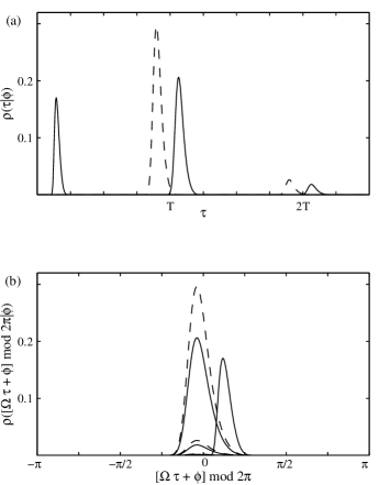
FIG. 1.: (a) Conditional ISI distributions for $\phi=-\pi/6$ (solid) and $\phi=\pi/6$ (dashed); other parameters $\mu=0.95$, $q=0.048$, $\Omega=0.05\pi$, $D=6\cdot 10^{-5}$. $T=40$ is the stimulus period. The refractory mode at small $\tau$ is present only for $\phi=-\pi/6$. The small modes around $2T$ correspond to the probability of skipping a period. (b) The same distributions as in (a), but now plotted vs. phase, $\psi=[\Omega\tau+\phi]\bmod 2\pi$, shifted to $[-\pi,\pi]$. The modes at $\approx-\pi/25$ coincide for the first and second stimulus period, while the refractory mode is clearly set apart.

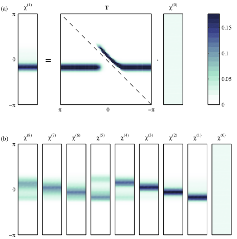
FIG. 2.: (a) Graphic representation of the Markov chain iteration given by Eq. (13). The dashed line is the matrix diagonal. Probability is given by grayscale as indicated by the colorbar. (b) Evolution of an initially uniform phase distribution under subsequent multiplications with T, from right to left. See text for details. Stimulus parameters: $\mu=0.95$, $q=0.05$, $\Omega=0.02\pi$, $D=1.3\cdot 10^{-4}$.

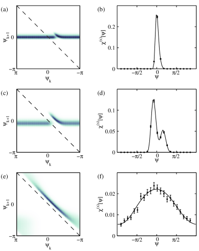
FIG. 3.: Phase transition matrices ${\bf T}$ (a, c, e) and corresponding stationary phase distributions $\mathchoice{{\hbox{\boldmath$\displaystyle\chi$}}}{{\hbox{\boldmath$\textstyle\chi$}}}{{\hbox{\boldmath$\scriptstyle\chi$}}}{{\hbox{\boldmath$\scriptscriptstyle\chi$}}}^{(s)}$ (b, d, f) for stimulus frequency $\Omega=0.05\pi$ at three different noise intensities $D=6.2\cdot 10^{-6}$ (a, b), $D=7.0\cdot 10^{-5}$ (c, d), and $D=4.8\cdot 10^{-3}$ (e, f); other parameters: $\mu=0.95$, $q=0.05$. The grayscale is the same for all matrices, white indicating vanishing probability. Error bars in the phase distributions indicate standard error of mean from simulated trains of 20,000 spikes. Observe the different scalings of the ordinate.

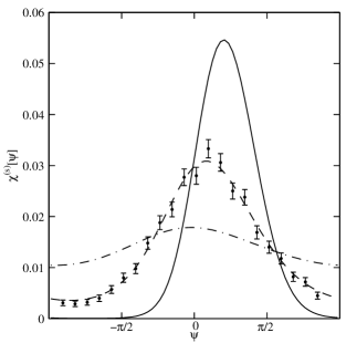
FIG. 4.: Stationary phase distributions $\mathchoice{{\hbox{\boldmath$\displaystyle\chi$}}}{{\hbox{\boldmath$\textstyle\chi$}}}{{\hbox{\boldmath$\scriptstyle\chi$}}}{{\hbox{\boldmath$\scriptscriptstyle\chi$}}}^{(s)}$ for stimulus frequency $\Omega=0.5\pi$ and noise intensities $D=7.8\cdot 10^{-4}$ (solid), $D=4.8\cdot 10^{-3}$ (dashed), and $D=3.0\cdot 10^{-2}$ (dash-dotted). Everything else is as in Fig. 3.

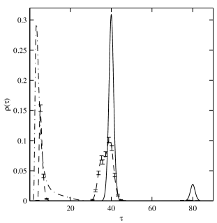
FIG. 5.: Stationary ISI distributions for slow stimuli. Noise intensities are $D=6.2\cdot 10^{-6}$ (solid), $D=7.0\cdot 10^{-5}$ (dashed), and $D=4.8\cdot 10^{-3}$ (dash-dotted). All other parameters are as in Fig. 3, error bars again indicate simulation results.

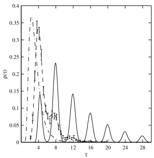
FIG. 6.: Stationary ISI distributions for fast stimuli. Noise intensities are $D=7.8\cdot 10^{-4}$ (solid), $D=4.8\cdot 10^{-3}$ (dashed), and $D=3.0\cdot 10^{-2}$ (dash-dotted). All parameters are as in Fig. 4, and error bars are from simulations.

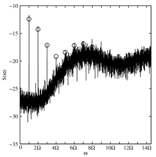
FIG. 7.: Power spectral density from an observation time of $T_{o}=200$ for the same stimulus as in Fig. 3(b, e). Circles indicate results at stimulus harmonics from the Markov chain analysis, while the drawn out line is obtained by FFT from a simulated train of 20,000 spikes. Ticks on the abscissa mark multiples of the stimulus period $\Omega=0.05\pi$.

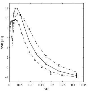
FIG. 8.: Signal-to-noise ratio vs. noise amplitude for three different stimulus frequencies: $\Omega=0.1\pi$ (dashed), $\Omega=0.33\pi$ (solid) and $\Omega=0.5\pi$ (dash-dotted). Other parameters are $\mu=0.95$ and $q=0.05$. Error bars show s.e.m. from simulated trains of 20,000 spikes.

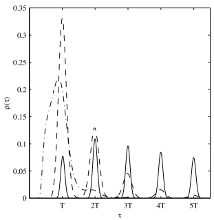
FIG. 9.: Inter-spike-interval distributions for the resonance frequency $\Omega_{r}$ and three noise intensities $D=1.3\cdot 10^{-4}$ (solid), $D=7.8\cdot 10^{-4}$ (dashed) and $D=4.8\cdot 10^{-3}$ (dash-dotted); other parameters $\mu=0.95$, $q=0.05$.

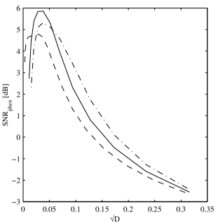
FIG. 10.: Signal-to-noise ratio from the phenomenological model of Eq. (22). All parameters are as in Fig. 8, with stimulus frequencies $\Omega=0.1\pi$ (dashed), $\Omega=0.33\pi$ (solid) and $\Omega=0.5\pi$ (dash-dotted).

REFERENCES

- [1] R. Benzi, A. Sutera, and A. Vulpiani, J Phys A 14, L453 (1981).
- [2] L. Gammaitoni, P. Hänggi, P. Jung, and F. Marchesoni, Rev Mod Phys 70, 223 (1998).
- [3] A. Longtin, J Stat Phys 70, 309 (1993).
- [4] K. Wiesenfeld and F. Moss, Nature 373, 33 (1995).
- [5] J. E. Levin and J. P. Miller, Nature 380, 165 (1996).
- [6] J. J. Collins, T. T. Imhoff, and P. Grigg, J Neurophysiology 76, 642 (1996).
- [7] P. Cordo et al., Nature 383, 769 (1996).
- [8] S. M. Bezrukov and I. Vodyanoy, Biophys J 73, 2456 (1997).
- [9] J. K. Douglass, L. Wilkens, E.Pantazelou, and F. Moss, Nature 365, 337 (1993).
- [10] M. Stemmler, M. Usher, and E. Niebur, Science 269, 1877 (1995).
- [11] F. Moss and D. F. Russell, Animal behavior enhanced by noise, Computational Neuroscience Meeting ’98, Santa Barbara, CA, July 1998.
- [12] J. G. Nicholls, A. R. Martin, and B. G. Wallace, From Neuron to Brain, 3 ed. (Sinauer, Sunderland, Mass., 1992).
- [13] H. C. Tuckwell, Stochastic Processes in the Neurosciences (SIAM, Philadelphia, 1989).
- [14] A. R. Bulsara et al., Phys Rev E 53, 3958 (1996).
- [15] H. E. Plesser and S. Tanaka, Phys Lett A 225, 228 (1997).
- [16] B. McNamara and K. Wiesenfeld, Phys Rev A 39, 4854 (1989).
- [17] P. Jung, Physics Reports 234, 175 (1993).
- [18] T. Zhou, F. Moss, and P. Jung, Phys Rev A 42, 3161 (1990).
- [19] A. Bulsara et al., J theor Biol 152, 531 (1991).
- [20] Z. Gingl, L. B. Kiss, and F. Moss, Europhys. Lett. 29, 191 (1995).
- [21] P. Jung, Phys Rev E 50, 2513 (1994).
- [22] K. Wiesenfeld et al., Phys Rev Lett 72, 2125 (1994).
- [23] D. R. Cox and P. A. W. Lewis, The Statistical Analysis of Series of Events (Methuen, London, 1966).
- [24] P. Lánský, Phys Rev E 55, 2040 (1997).
- [25] R. Kempter, W. Gerstner, J. L. van Hemmen, and H. Wagner, Neural Computation 10, 1987 (1998).
- [26] N. G. van Kampen, Stochastic Processes in Physics and Chemistry, 2nd ed. (North-Holland, Amsterdam, 1992).
- [27] P. Linz, Analytical and Numerical Methods for Volterra Equations (SIAM, Philadelphia, 1985).
- [28] C. T. H. Baker, The Numerical Treatment of Integral Equations (Clarendon Press, Oxford, 1977).
- [29] R. von Mises, Mathematical Theory of Probability and Statistics (Academic Press, New York, 1964), ed. by H. Geiringer.
- [30] J. Mogdans, private communication.
- [31] J. E. Rose, J. F. Brugge, D. J. Anderson, and J. E. Hind, J Neurophysiology 30, 769 (1967).
- [32] R. A. Lavine, J Neurophysiology 34, 467 (1971).
- [33] D. T. Gillespie, Phys Rev E 54, 2084 (1996).
- [34] M. Stemmler, Network 7, 687 (1996).
- [35] M. B. Priestley, Spectral Analysis and Time Series (Academic Press, London, 1996).
- [36] J. Franklin and W. Bair, SIAM J Appl Math 55, 1074 (1995).
- [37] W. Bair, C. Koch, W. Newsome, and K. Britten, J Neuroscience 14, 2870 (1994).
- [38] L. Gammaitoni, Phys Rev E 52, 4691 (1995).
- [39] J. M. Goldberg and P. B. Brown, J Neurophysiology 32, 613 (1969).
- [40] H. E. Plesser and W. Gerstner, submitted.
- [41] L. Gammaitoni, F. Marchesoni, and S. Santucci, Phys Rev Lett 74, 1052 (1995).
- [42] V. Berdichevsky and M. Gitterman, J Phys A 29, L447 (1996).
- [43] M. H. Choi, R. F. Fox, and P. Jung, Phys Rev E 57, 6335 (1998).
- [44] W. Gerstner, R. Kemptner, J. L. van Hemmen, and H. Wagner, Nature 383, 76 (1996).