Estimating probability densities from short samples:
a parametric maximum likelihood approach

Abstract

A parametric method similar to autoregressive spectral estimators is proposed to determine the probability density function (pdf) of a random set. The method proceeds by maximizing the likelihood of the pdf, yielding estimates that perform equally well in the tails as in the bulk of the distribution. It is therefore well suited for the analysis short sets drawn from smooth pdfs and stands out by the simplicity of its computational scheme. Its advantages and limitations are discussed.

I Introduction

There are many applications in which it is necessary to estimate the probability density function (pdf) from a finite sample of $n$ observations $\{x_{1},\,x_{2},\,\ldots,\,x_{n}\}$ whose true pdf is $f(x)$. Here we consider the generic case in which the identically distributed (but not necessarily independent) random variables have a compact support $x_{k}\in[a,b]$.

The usual starting point for a pdf estimation is the naive estimate

$$\hat{f}_{\delta}(x)=\frac{1}{n}\sum_{i=1}^{n}\delta(x-x_{i})\ ,$$ (1)

where $\delta(.)$ stands for the Dirac delta function. Although this definition has a number of advantages, it is useless for practical purposes since a smooth functional is needed.

Our problem consists in finding an estimate $\hat{f}(x)$ whose integral over an interval of given length converges toward that of the true pdf as $n\rightarrow\infty$. Many solutions have been developed for that purpose: foremost among these are kernel techniques in which the estimate $\hat{f}_{\delta}(x)$ is smoothed locally using a kernel function $K(x)$ [3, 4, 5]

$$\hat{f}(x)=\int_{a}^{b}\frac{1}{w}K\left(\frac{x-y}{w}\right)\,\hat{f}_{\delta}(y)\,{\rm d}y\ ,$$ (2)

whose width is controlled by the parameter $w$. The well-known histogram is a variant of this technique. Although kernel approaches are by far the most popular ones, the choice of a suitable width remains a basic problem for which visual guidance is often needed. More generally, one faces the problem of choosing a good partition. Some solutions include Bayesian approaches [6], polynomial fits [7] and methods based on wavelet filtering [8].

An alternative approach, considered by many authors [9, 10, 11, 12, 13], is a projection of the pdf on orthogonal functions

$$\hat{f}(x)=\sum_{k}\alpha_{k}\;g_{k}(x)\ ,$$ (3)

where the partition problem is now treated in dual space. This parametric approach has a number of interesting properties: a finite expansion often suffices to obtain a good approximation of the pdf and the convergence of the series versus the sample size $n$ is generally faster than for kernel estimates. A strong point is its global character, since the pdf is fitted globally, yielding estimates that are better behaved in regions where the lack of statistics causes kernel estimates to perform poorly. Such a property is particularly relevant for the analysis of turbulent wavefields, in which the tails of the distribution are of great interest (e.g. [14]).

These advantages, however, should be weighed against a number of downsides. Orthogonal series do not provide consistent estimates of the pdf since for increasing number of terms they converge toward $\hat{f}_{\delta}(x)$ instead of the true density $f(x)$ [15]. Furthermore, most series can only handle continuous or piecewise continuous densities. Finally, the pdf estimates obtained that way are not guaranteed to be nonnegative (see for example the problems encountered in [16]).

The first problem is not a major obstacle, since most experimental distributions are smooth anyway. The second one is more problematic. In this paper we show how it can be partly overcome by using a Fourier series expansion of the pdf and seeking a maximization of the likelihood

$$\hat{L}=\int_{a}^{b}\log\hat{f}(x)\;{\rm d}x\ .$$ (4)

The problem of choosing an appropriate partition then reduces to that of fitting the pdf with a positive definite Padé approximant [17].

Our motivation for presenting this particular parametric approach stems from its robustness, its simplicity and the originality of the computational scheme it leads to. The latter, as will be shown later, is closely related to the problem of estimating power spectral densities with autoregressive (AR) or maximum entropy methods [18, 19, 20]. To the best of our knowledge, the only earlier reference to similar work is that by Carmichael [21]; here we emphasize the relevance of the method for estimating pdfs and propose a criterion for choosing the optimum number of basis functions.

II The Maximum likelihood approach

The method we now describe basically involves a projection of the pdf on a Fourier series. The correspondence between the continuous pdf $f(x)$ and its discrete characteristic function $\phi_{k}$ is established by [22]

$$\phi_{k} = \int_{-\pi}^{+\pi}f(x)\;e^{jkx}\;{\rm d}x$$ (5)

$$f(x) = 2\pi\sum_{k=-\infty}^{+\infty}\phi_{k}\;e^{-jkx}\ ,$$ (6)

where $\phi_{k}=\phi_{-k}^{*}\in{{\sf C\rule{0.6458pt}{5.59721pt}\hskip 3.87495pt}}$ is hermitian [23]. Note that we have applied a linear transformation to convert the support from $[a,b]$ to $[-\pi,\pi]$.

For a finite sample, an unbiased estimate of the characteristic function is obtained by inserting eq. 1 into eq. 5, giving

$$\hat{\phi}_{k}=\frac{1}{n}\sum_{i=1}^{n}e^{jkx_{i}}\ .$$ (7)

The main problem now consists in recovering the pdf from eq. 6 while avoiding the infinite summation. By working in dual space we have substituted the partition choice problem by that of selecting the number of relevant terms in the Fourier series expansion.

The simplest choice would be to truncate the series at a given “wave number” $p$ and discard the other ones

$$\hat{f}(x)=2\pi\sum_{k=-p}^{+p}\hat{\phi}_{k}\;e^{-jkx}\ .$$ (8)

Such a truncation is equivalent to keeping the lowest wave numbers and thus filtering out small details of the pdf. Incidentally, this solution is equivalent to a kernel filtering with $K(x)=\sin(\pi x)/\pi x$ as kernel. This kernel is usually avoided because it suffers from many drawbacks such as the generation of spurious oscillations.

An interesting improvement was suggested by Burg in the context of spectral density estimation (see for example [18, 19]). The heuristic idea is to keep some of the low wave number terms while the remaining ones, instead of being set to zero, are left as free parameters:

$$\hat{f}(x)=2\pi\sum_{k=-\infty}^{+\infty}\hat{\alpha}_{k}\;e^{-jxk}$$ (9)

$$\mbox{with}\ \ \hat{\alpha}_{k}=\hat{\phi}_{k},\ \ \ |k|\leq p\ .$$ (10)

The parameters $\hat{\alpha}_{k}$, for $|k|>p$, are then fixed self-consistently according to some criterion.

We make use of this freedom to constrain the solution to a particular class of estimates. Without any prior information at hand, a reasonable choice is to select the estimate that contains the least possible information or is the most likely. It is therefore natural to seek a maximization of an entropic quantity such as the sample entropy

$$\hat{H}=-\int_{-\pi}^{+\pi}\hat{f}(x)\log\hat{f}(x)\;{\rm d}x\ ,$$ (11)

or the sample likelihood

$$\hat{L}=\int_{-\pi}^{+\pi}\log\hat{f}(x)\;{\rm d}x\ .$$ (12)

We are a priori inclined to choose the entropy because our objective is the estimation of the pdf and not that of the characteristic function. However, numerical investigations done in the context of spectral density estimation rather lend support to the likelihood criterion [24]. A different and stronger motivation for preferring a maximization of the likelihood comes from the simplicity of the computational scheme it gives rise to.

This maximization means that the tail of the characteristic function is chosen subject to the constraint

$$\frac{\partial\hat{L}}{\partial\hat{\alpha}_{k}}=0,\ \ \ |k|>p\ .$$ (13)

From eqs. 9 and 12 the likelihood can be rewritten as

$$\hat{L}=\int_{-\pi}^{+\pi}\log\left(2\pi\sum_{k=-\infty}^{+\infty}\hat{\alpha}_{k}\;e^{-jxk}\right)\,{\rm d}x\ .$$ (14)

As shown in the appendix, the likelihood is maximized when the pdf can be expressed by the functional

$$\hat{f}_{p}(x)=\frac{1}{\sum_{k=-p}^{p}c_{k}e^{-jkx}}\ ,$$ (15)

which is a particular case of a Padé approximant with poles only and no zeros [17]. Requiring that $\hat{f}_{p}(x)$ is real and bounded, it can be rewritten as

$$\hat{f}_{p}(x)=\frac{\varepsilon_{0}}{2\pi}\,\frac{1}{\left|1+a_{1}e^{-jx}+\cdots+a_{p}e^{-jpx}\right|^{2}}\ .$$ (16)

The values of the coefficients $\{a_{1},\ldots,a_{p}\}$ and of the normalization constant $\varepsilon_{0}$ are set by the condition that the Fourier transform of $\hat{f}_{p}(x)$ must match the sample characteristic function $\hat{\phi}_{k}$ for $|k|\leq p$.

This solution has a number of remarkable properties, some of which are deferred to the appendix. Foremost among these are its positive definite character and the simple relationship which links the polynomial coefficients $\{a_{1},\ldots,a_{p}\}$ to the characteristic function on which they perform a regression. Indeed, we have

$$\hat{\phi}_{k}+a_{1}\hat{\phi}_{k-1}+a_{2}\hat{\phi}_{k-2}+\cdots+a_{p}\hat{\phi}_{k-p}= 0$$ , (17)

$$1\leq k\leq p \ .$$ (18)

This can be cast in a set of Yule-Walker equations whose unique solution contains the polynomial coefficients

$$\left[\begin{array}[]{cccc}\hat{\phi}_{0}&\hat{\phi}_{-1}&\cdots&\hat{\phi}_{-p+1}\\ \hat{\phi}_{1}&\hat{\phi}_{0}&\cdots&\hat{\phi}_{-p+2}\\ \vdots&\vdots&&\vdots\\ \hat{\phi}_{p-1}&\hat{\phi}_{p-2}&\cdots&\hat{\phi}_{0}\end{array}\right]\;\left[\begin{array}[]{c}a_{1}\\ a_{2}\\ \vdots\\ a_{p}\end{array}\right]=-\left[\begin{array}[]{c}\hat{\phi}_{1}\\ \hat{\phi}_{2}\\ \vdots\\ \hat{\phi}_{p}\end{array}\right]\ .$$ (19)

Advantage can be taken here of the Toeplitz structure of the matrix. The proper normalization ($\int_{-\pi}^{+\pi}\hat{f}(x)\,{\rm d}x=1$) of the pdf is ensured by the value of $\varepsilon_{0}$, which is given by a variant of eq. 17

$$\hat{\phi}_{0}+a_{1}\hat{\phi}_{-1}+a_{2}\hat{\phi}_{-2}+\cdots+a_{p}\hat{\phi}_{-p}=\varepsilon_{0}\ .$$ (20)

Equations 16 and 19 illustrate the simplicity of the method.

III Some properties

A clear advantage of the method over conventional series expansions is the automatic positive definite character of the pdf. Another asset is the close resemblance with autoregressive or maximum entropy methods that are nowadays widely used in the estimation of spectral densities. Both methods have in common the estimation of a positive function by means of a Padé approximant whose coefficients directly issue from a regression (eq. 17). This analogy allows us to exploit here some results previously obtained in the framework of spectral analysis.

One of these concerns the statistical properties of the maximum likelihood estimate. These properties are badly known because the nonlinearity of the problem impedes any analytical treatment. The analogy with spectral densities, however, reveals that the estimates are asymptotically normally distributed with a standard deviation [25, 26]

$$\sigma_{\hat{f}}\propto\hat{f}\ .$$ (21)

This scaling should be compared against that of conventional kernel estimates, for which

$$\sigma_{\hat{f}}\propto\sqrt{\hat{f}}\ .$$ (22)

The key point is that kernel estimates are relatively less reliable in low density regions than in the bulk of the distribution, whereas the relative uncertainty of maximum likelihood estimates is essentially constant. The latter property is obviously preferable when the tails of the distribution must be investigated, e.g. in the study of rare events.

Some comments are now in order. By choosing a Fourier series expansion, we have implicitly assumed that the pdf was $2\pi$-periodic, which is not necessarily the case. Thus special care is needed to enforce periodicity, since otherwise wraparound may result [27]. The solution to this problem depends on how easily the pdf can be extended periodically. In most applications, the tails of the distribution progressively decrease to zero, so periodicity may be enforced simply by artificially padding the tails with a small interval in which the density vanishes. We do this by rescaling the support from $[a,b]$ to an interval which is slightly smaller than $2\pi$, say $[-3,3]$ [28]. Once the Padé approximant is known, the $[-3,3]$ interval is scaled back to $[a,b]$.

If there is no natural periodic extension to the pdf, (for example if $f(a)$ strongly differs from $f(b)$) then the choice of Fourier basis functions in eq. 3 becomes questionable and, not surprisingly, the quality of the fit degrades. Even in this case, however, the results can still be improved by using ad hoc solutions [29].

We mentioned before that the maximum likelihood method stands out by computational simplicity. Indeed, a minimization of the entropy would lead to the solution

$$\log\hat{f}_{p}(x)\propto\sum_{k=-p}^{p}c_{k}e^{-jkx}\ ,$$ (23)

whose numerical implementation requires an iterative minimization and is therefore considerably more demanding.

Finally, the computational cost is found to be comparable or even better (for large sets) than for conventional histogram estimates. Most of the computation time goes into the calculation of the characteristic function, for which the number of operations scales as the sample size $n$.

IV Choosing the order of the model

The larger the order $p$ of the model is, the finer the details in the pdf estimate are. Finite sample effects, however, also increase with $p$. It is therefore of prime importance to find a compromise. Conventional criteria for selecting the best compromise between model complexity and quality of the fit, such as the Final Prediction Error and the Minimum Description Length [18, 19, 20] are not applicable here because they require the series of characteristic functions $\{\phi_{k}\}$ to be normally distributed, which they are not.

Guided by the way these empirical criteria have been chosen, we have defined a new one, which is based on the following observation: as $p$ increases starting from 0, the pdfs $\hat{f}_{p}(x)$ progressively converge toward a stationary shape; after some optimal order, however, ripples appear and the shapes start diverging again. It is therefore reasonable to compare the pdfs pairwise and determine how close they are. A natural measure of closeness between two positive distributions $\hat{f}_{p}(x)$ and $\hat{f}_{p+1}(x)$ is the Kullback-Leibler entropy or information gain [30, 31]

$$\hat{I}(\hat{f}_{p+1},\hat{f}_{p})=\int_{-\pi}^{+\pi}\,\hat{f}_{p+1}(x)\,\log\frac{\hat{f}_{p+1}(x)}{\hat{f}_{p}(x)}\;{\rm d}x\ ,$$ (24)

which quantifies the amount of information gained by changing the probability density describing our sample from $\hat{f}_{p}$ to $\hat{f}_{p+1}$. In other words, if $H_{p}$ (or $H_{p+1}$) is the hypothesis that $x$ was selected from the population whose probability density is $\hat{f}_{p}$ ($\hat{f}_{p+1}$), then $\hat{I}(\hat{f}_{p+1},\hat{f}_{p})$ is given as the mean information for discriminating between $H_{p+1}$ and $H_{p}$ per observation from $\hat{f}_{p+1}$  [30].

Notice that the information gain is not a distance between distributions; it nevertheless has the property of being non negative and to vanish if and only if $\hat{f}_{p}\equiv\hat{f}_{p+1}$. We now proceed as follows : starting from $p=0$ the order is incremented until the information gain reaches a clear minimum; this corresponds, as it has been checked numerically, to the convergence toward a stationary shape; the corresponding order is then taken as the requested compromise. Clearly, there is some arbitrariness in the definition of a such a minimum since visual inspection and common sense are needed. In most cases, however, the solution is evident and the search can be automated. Optimal orders usually range between 2 and 10; larger values may be needed to model discontinuous or complex shaped densities.

V Some examples

Three examples are now given in order to illustrate the limits and the advantages of the method.

A General properties

First, we consider a normal distribution with exponential tails as often encountered in turbulent wavefields. We simulated a random sample with $n=2000$ elements and the main results appear in Fig. 1.

The information gain (Fig. 1b) decreases as expected until it reaches a well defined minimum at $p=7$, which therefore sets the optimal order of our model. Since the true pdf is known, we can test this result against a common measure of the quality of the fit, which is the Mean Integrated Squared Error (MISE)

$${\rm MISE}(p)=\int_{a}^{b}[f(x)-\hat{f}_{p}(x)]^{2}{\rm d}x\ .$$ (25)

The MISE, which is displayed in Fig. 1b, also reaches a minimum at $p=8$ and thus supports the choice of the information gain as a reliable indicator for the best model. Tests carried out on other types of distributions confirm this good agreement.

Now that the optimum pdf has been found, its characteristic function can be computed and compared with the measured one, see Fig. 1a. As expected, the two characteristic functions coincide for the $p$ lowest wave numbers (eq. 17); they diverge at higher wave numbers, for which the model tries to extrapolate the characteristic function self-consistently. The fast falloff of the maximum likelihood estimate explains the relatively smooth shape of the resulting pdf.

Finally, the quality of the pdf can be visualized in Fig. 1d, which compares the measured pdf with the true one, and an estimate based on a histogram with 101 bins. An excellent agreement is obtained, both in the bulk of the distribution and in the tails, where the exponential falloff is correctly reproduced. This example illustrates the ability of the method to get reliable estimates in regions where standard histogram approaches have a lower performance.

B Interpreting the characteristic function

The shape of the characteristic function in Fig. 1a is reminiscent of spectral densities consisting of a low wave number (band-limited) component embedded in broadband noise. A straightforward calculation of the expectation of $|\phi_{k}|$ indeed reveals the presence of a bias which is due to the finite sample size

$${\rm E}[|\hat{\phi}_{k}|]=|\phi_{k}|+\frac{\gamma}{\sqrt{n}}\ ,$$ (26)

where $\gamma$ depends on the degree of independence between the samples in $\{x\}$. This bias is illustrated in Fig. 2 for independent variables drawn from a normal distribution, showing how the wave number resolution gradually degrades as the sample size decreases. Incidentally, a knowledge of the bias level could be used to obtain confidence intervals for the pdf estimate. This would be interesting insofar no assumptions have to be made on possible correlations in the data set. We found this approach, however, to be too inaccurate on average to be useful.

The presence of a bias also gives an indication of the smallest scales (in terms of amplitude of $x$) one can reliably distinguish in the pdf. For a set of 2000 samples drawn from a normal distribution, for example, components with wave numbers in excess of $k=3$ are hidden by noise and hence the smallest meaningful scales in the pdf are of the order of $\delta x=0.33$. These results could possibly be further improved by Wiener filtering.

C Influence of the sample size

To investigate the effect of the sample length $n$, we now consider a bimodal distribution consisting of two normal distributions with different means and standard deviations. Such distributions are known to be difficult to handle with kernel estimators.

Samples with respectively $n=200$, $n=2000$ and $n=20000$ elements were generated; their characteristic functions and the resulting pdfs are displayed in Fig. 3. Clearly, finite sample effects cannot be avoided for small samples but the method nevertheless succeeds relatively well in capturing the true pdf and in particular the small peak associated with the narrow distribution. An analysis of the MISE shows that it is systematically lower for maximum likelihood estimates than for standard histogram estimates, supporting the former.

D A counterexample

The previous examples gave relatively good results because the true distributions were rather smooth. Although such smooth distributions are generic in most applications it may be instructive to look at a counterexample, in which the method fails.

Consider the distribution which corresponds to a cut through an annulus

$$f(x)=\left\{\begin{tabular}[]{cl}$\frac{1}{2}$&$1\leq|x|\leq 2$\\ 0&elsewhere\\ \end{tabular}\right.\ .$$ (27)

A sample was generated with $n=2000$ elements and the resulting information gains are shown in Fig. 4. There is an ambiguity in the choice of the model order and indeed the convergence of the pdf estimates toward the true pdf is neither uniform nor in the mean. Increasing the order improves the fit of the discontinuity a little but also increases the oscillatory behavior known as the Gibbs phenomenon. This problem is related to the fact that the pdf is discontinuous and hence the characteristic function is not absolutely summable.

Similar problems are routinely encountered in the design of digital filters, where steep responses cannot be approximated with infinite impulse response filters that have a limited number of poles [22]. The bad performance of the maximum likelihood approach in this case also comes from its inability to handle densities that vanish over finite intervals. A minimization of the entropy would be more appropriate here.

VI Conclusion

We have presented a parametric procedure for estimating univariate densities using a positive definite functional. The method proceeds by maximizing the likelihood of the pdf subject to the constraint that the characteristic functions of the sample and estimated pdfs coincide for a given number of terms. Such a global approach to the estimation of pdfs is in contrast to the better known local methods (such as non-parametric kernel methods) whose performance is poorer in regions where there is a lack of statistics, such as the tails of the distribution. This difference makes the maximum likelihood method relevant for the analysis of short records (with typically hundreds or thousands of samples). Other advantages include a simple computational procedure that can be tuned with a single parameter. An entropy-based criterion has been developed for selecting the latter.

The method works best with densities that are at least once continuously differentiable and that can be extended periodically. Indeed, the shortcomings of the method are essentially the same as for autoregressive spectral estimates, which give rise to the Gibbs phenomenon if the density is discontinuous.

The method can be extended to multivariate densities, but the computational procedures are not yet within the realm of practical usage. Its numerous analogies with the design of digital filters suggest that it is still open to improvements.

We detail here the main stages that lead to the pdf estimate described in Sec. II because extensive proofs are rather difficult to find in the literature.

The maximum likelihood condition (eq. 13) can be expressed as

$$\int_{-\pi}^{+\pi}\frac{e^{-jkx}}{\sum_{l=-\infty}^{\infty}\hat{\alpha}_{l}e^{-jlx}}\,{\rm d}x=\int_{-\pi}^{+\pi}\frac{e^{-jkx}}{\hat{f}(x)}\,{\rm d}x=0\ ,$$ (28)

for $|k|>p$ [32]. This simply means that the Fourier expansion of $\left(\hat{f}(x)\right)^{-1}$ should not contain terms of order $|k|>p$ and hence the solution must be

$$\hat{f}_{p}(x)=\frac{1}{\sum_{k=-p}^{p}c_{k}e^{-jkx}}\ .$$ (29)

The pdf we are looking for must of course be real, and so the coefficients should be hermitian $c_{k}=c_{-k}^{*}$. We also want the pdf to be bounded, which implies that

$$\sum_{k=-p}^{p}c_{k}e^{-jkx}\neq 0\ ,\ \ \ \forall x\in[-\pi,\pi]\ .$$ (30)

Let us now define, for $z$ complex

$$C(z)=\sum_{k=-p}^{p}c_{-k}z^{k}\ ,$$ (31)

and

$$P(z)=z^{p}C(z)\ .$$ (32)

$P(z)$ is a polynomial of degree $2p$. It can be easily verified that [33]

$$P(z)=z^{2p}\left[P\left(\frac{1}{z^{*}}\right)\right]^{*}\,$$ (33)

as a consequence of the hermiticity of the coefficients $c_{k}$. In particular, this tells us that if $z_{1}$ is a root of $P(z)$, then $1/z_{1}^{*}$ (the complex-conjugate of its mirror image with respect to the unit circle) is also a root of $P(z)$. From eq. 30 we know that none of these roots are located on the unit circle.

Let us now rearrange the roots of $P(z)$, denoting by $\{z_{1},\ldots,z_{p}\}$ the $p$ roots lying outside the unit disk and by $\{1/z_{1}^{*},\ldots,1/z_{p}^{*}\}$ the $p$ other ones that are located inside the unit circle. We can then write:

$$P(z)=c_{-p}(z-z_{1})\cdots(z-z_{p})\left(z-\frac{1}{z_{1}^{*}}\right)\cdots\left(z-\frac{1}{z_{p}^{*}}\right)\ ,$$ (34)

with

$$c_{-p}z_{1}\cdots z_{p}=c_{p}z_{1}^{*}\cdots z_{p}^{*}\ .$$ (35)

From this $C(z)$ can be written as:

$$C(z)=\pm B(z)\left[B\left(\frac{1}{z^{*}}\right)\right]^{*}\ ,$$ (36)

where

$$B(z)=\left|\frac{c_{p}}{z_{1}\cdots z_{p}}\right|^{\frac{1}{2}}(z-z_{1})\cdots(z-z_{p})\ .$$ (37)

By construction, all the roots of $B(z)$ are located outside the unit disk.

Finally, we get for $\hat{f}_{p}(x)$:

$$\hat{f}_{p}(x)=\frac{1}{C(z=e^{jx})}=\pm\frac{1}{\left|B(e^{jx})\right|^{2}}\ .$$ (38)

All the solutions of the maximum likelihood principle, if real and bounded, are thus of constant sign and have the structure given by eq. 38. Excluding negative definite solutions we obtain

$$\hat{f}_{p}(x)=\frac{\varepsilon_{0}}{2\pi}\,\frac{1}{\left|1+a_{1}e^{-jx}+\cdots+a_{p}e^{-jpx}\right|^{2}}\ ,$$ (39)

where

$$\varepsilon_{0}=\frac{2\pi}{|b_{0}|^{2}}\ ,\ \ \ a_{i}=\frac{b_{i}^{*}}{b_{0}^{*}}\ ,\ \ \ i=1,\cdots,p\ ,$$ (40)

where $\{b_{1},\ldots,b_{p}\}$ are the coefficients of the polynomial $B(z)$ and $A(z)=1+a_{1}z+\cdots+a_{p}z^{p}$ has all its roots outside the unit disk. The normalization constant $\varepsilon_{0}$ is set by the condition

$$\int_{-\pi}^{+\pi}\hat{f}_{p}(x)\,{\rm d}x=1\ .$$ (41)

The coefficients $\{a_{1},\ldots,a_{p}\}$ are now identified on the basis that the characteristic function of the pdf estimate $\hat{f}_{p}(x)$ should match the first $p$ terms of the sample characteristic function exactly, namely

$$\hat{\alpha}_{k}=\hat{\phi}_{k}=\int_{-\pi}^{+\pi}\hat{f}_{p}(x)\;e^{jkx}{\rm d}x\ ,\ \ \ 1\leq k\leq p\ .$$ (42)

To this purpose, let us compute the quantity $\sum_{k=0}^{p}a_{k}\hat{\alpha}_{l-k}$. Recalling that $A(z)$ is analytic in the unit circle and making use of Cauchy’s residue theorem, we obtain

$$\sum_{k=0}^{p} a_{k}\hat{\phi}_{l-k}=0\ ,\ \ 1\leq l\leq p$$ (43)

$$\sum_{k=0}^{p} a_{k}\hat{\phi}_{-k}=\varepsilon_{0}\ .$$ (44)

Equation 43 fixes the values of $\{a_{1},\ldots,a_{p}\}$ and gives the Yule-Walker equations (eq. 19). The solution is unique provided that

$$\det\left[\begin{array}[]{ccc}\hat{\phi}_{0}&\cdots&\hat{\phi}_{-p+1}\\ \vdots&&\vdots\\ \hat{\phi}_{p-1}&\cdots&\hat{\phi}_{0}\end{array}\right]\neq 0\ .$$ (45)

The latter condition is verified except when a repetitive pattern occurs in the characteristic function. In this happens then the order $p$ should simply be chosen to be less than the periodicity of this pattern.

Besides its positivity, the solution we obtain has a number of useful properties. First, note that all the terms of its characteristic function can be computed recursively by

$$\left[\begin{array}[]{c}\hat{\alpha}_{k+1}\\ \hat{\alpha}_{k}\\ \vdots\\ \hat{\alpha}_{k-p+2}\end{array}\right]\,=\,\left[\begin{array}[]{cccc}-a_{1}&-a_{2}&\cdots&-a_{p}\\ 1&0&\cdots&0\\ 0&1&\cdots&0\\ \vdots&\vdots&&\vdots\\ 0&0&\cdots&0\end{array}\right]\,\left[\begin{array}[]{c}\hat{\alpha}_{k}\\ \hat{\alpha}_{k-1}\\ \vdots\\ \hat{\alpha}_{k-p+1}\end{array}\right]\,,$$ (46)

in which the starting condition is set by the $p$ first values of $\hat{\phi}_{k}$. From this recurrence relation the asymptotic behavior of $\hat{\phi}_{k}$ as $k\rightarrow\infty$ can be probed by diagonalizing the state space matrix in eq. 46. The eigenvalues of this matrix are the roots $\{1/z_{1}^{*},\cdots,1/z_{p}^{*}\}$ (called poles), which by construction are all inside the unit disk. Therefore

$$\lim_{k\rightarrow\infty}|\phi_{k}|\sim e^{\lambda k}\ ,$$ (47)

where $\lambda$ is related to the largest root and is always negative since

$$\lambda=\max_{k}\,\log\left|\frac{1}{z_{k}^{*}}\right|\ \ <\ \ 0\ .$$ (48)

This exponential falloff of the characteristic function explains why the resulting pdf is relatively smooth.

Now that we have found a solution in terms of a $[0,p]$ Padé approximant, it is legitimate to ask whether a $[q,p]$ approximant of the type

$$\hat{f}_{q,p}(x)=\frac{\left|d_{0}+d_{1}e^{-jx}+\cdots+d_{q}e^{-jqx}\right|^{2}}{\left|1+a_{1}e^{-jx}+\cdots+a_{p}e^{-jpx}\right|^{2}}$$ (49)

could not bring additional flexibility and hence provide a better estimate of the pdf. Again, we exploit the analogy with spectral density estimation, in which the equivalent of $[q,p]$ Padé approximants are obtained with autoregressive moving average (ARMA) models. The superiority of ARMA over AR models is generally agreed upon [34], although the MISE does not firmly establish it [19]. Meanwhile we note that there does not seem to exist a simple variational principle, similar to that of the likelihood maximization, which naturally leads to a $[q,p]$ Padé approximant of the pdf.

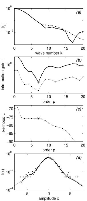
FIG. 1.: Example of a normal distribution with exponential tails. The sample size is $n=2000$. From top to bottom are shown: (a) the magnitude $|\hat{\phi}_{k}|$ of the characteristic function (thick line) and the fit resulting from an 7’th order model; (b) the information gain (thick line) and the MISE, both showing a minimum around $p=7$ which is marked by a circle; (c) the likelihood $\hat{L}$ associated with the different pdfs estimated for $p=$1–20; and finally (d) the maximum likelihood estimate of the pdf (thick line), an estimate based on a histogram with 101 equispaced bins (dots) and the true pdf (thin line).

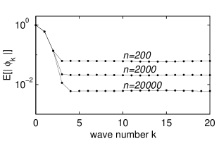
FIG. 2.: The expectation ${\rm E}[|\hat{\phi}_{k}|]$ computed for sets of various sizes taken from the same normal distribution. The noise-induced bias level goes down as the size increases, progressively revealing finer details of the pdf.

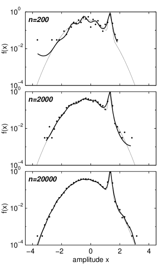
FIG. 3.: The pdfs as calculated for sets of various sizes taken from the same bi-normal distribution. The thick line designates the maximum likelihood estimate, the thin line the true pdf and the dots a histogram estimate obtained from 61 equispaced bins. The optimum orders are respectively from top to bottom $p=5$, $p=6$ and $p=11$.

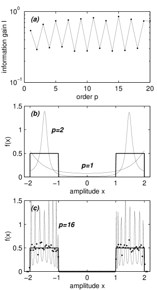
FIG. 4.: Results obtained for an annular distribution; the sample size is $n=2000$. In (a) The information gain has no clear minimum and hence there is no well defined order for the model. In (b) the estimated pdfs for $p=1$ and $p=2$ fail to fit the true pdf (thick line). Increasing the order (c) improves the fit but also enhances the Gibbs phenomenon. Dots correspond to a histogram estimate with equispaced bins.

REFERENCES

- [1] Université de Provence and CNRS, e-mail : ddwit@cpt.univ-mrs.fr
- [2] e-mail : floriani@cpt.univ-mrs.fr
- [3] R. A. Tapia and J. R. Thompson, Nonparametric probability density estimation (The Johns Hopkins University Press, Baltimore, 1978).
- [4] B. W. Silverman, Density estimation for statistics and data analysis (Chapman and Hall, London, 1986).
- [5] A. Izenman, JASA 86, 205–224 (1991).
- [6] D. H. Wolpert and D. R. Wolf, Phys. Rev. E 52, 6841–6854 (1995).
- [7] P. L. G. Ventzek and K. Kitamori, J. Appl. Phys. 75, 3785–3788 (1994).
- [8] D. L. Donoho, in Wavelet analysis and applications, Y. Meyer and S. Roques, eds. (Éditions Frontières, Gif-sur-Yvette, 1993) 109–128.
- [9] N. N. Čenkov, Soviet Math. Doklady 3, 1559–1562 (1962).
- [10] S. C. Schwartz, Ann. Math. Statist. 38, 1262–1265 (1967).
- [11] R. A. Kronmal and M. Tarter, J. Amer. Statist. Assoc. 63, 925–952 (1968).
- [12] B. R. Crain, Ann. Statist. 2, 454–463 (1974).
- [13] A. Pinheiro and B. Vidakovic, Comp. Stat. Data Analysis, in the press.
- [14] U. Frisch, Turbulence (Cambridge University Press, Cambridge, 1995).
- [15] L. Devroye and L. Györfi, Nonparametric density estimation, the view (Wiley, New York, 1985).
- [16] K. Nanbu, Phys. Rev. E 52, 5832–5838 (1995).
- [17] P. R. Graves-Morris, ed., Padé approximants (The Institute of Physics, London, 1972).
- [18] M. B. Priestley, Spectral analysis and time series (Academic Press, London, 1981).
- [19] S. Haykin, ed., Nonlinear methods for spectral analysis (Springer-Verlag, Berlin, 1979).
- [20] D. B. Percival and A. T. Walden, Spectral analysis for physical applications (Cambridge University Press, Cambridge, 1993).
- [21] J.-P. Carmichael, The autoregressive method: a method for approximating and estimating positive functions, Ph.D. dissert. (State Univ. of New York, Buffalo, 1976).
- [22] A. V. Oppenheim and R. W. Schafer, Discrete-time signal processing (Prentice-Hall, Englewood Cliffs NJ, 1989).
- [23] This is strictly speaking not the characteristic function, but its complex conjugate.
- [24] R. W. Johnson and J. E. Shore, Which is the better entropy expression for speech processing: or ? IEEE Trans. Acoust. Speech Signal Proc. 32, 129–137 (1984).
- [25] K. N. Berk, Ann. Statist. 2, 489-502 (1974).
- [26] E. Parzen, IEEE Trans. Autom. Control AC-19, 723-729 (1974).
- [27] J. D. Scargle, Astroph. J. 343, 874–887 (1989).
- [28] The width of the interval actually has little impact on the outcome as long as it is much less than . The width and its asymmetry could possibly be tailored to the pdf in order to improve the fit a little.
- [29] The simplest one consists in symmetrizing the pdf: the initial sample is transformed into a new one which is twice a large , and covers the interval . The pdf of this new sample is computed and one half of it is kept to obtain the desired result. This procedure doubles the volume of data, but the computational cost remains approximately the same since one half only of the data is actually needed to estimate the characteristic function.
- [30] S. Kullback and R. A. Leibler, Ann. Math. Stat. 22, 79-86 (1951).
- [31] C. Beck and F. Schlögl, Thermodynamics of chaotic systems (Cambridge University Press, Cambridge, 1993).
- [32] It can be readily verified that this solution indeed corresponds to a maximum.
- [33] D. E. Smylie, G. K. C. Clarke, T. J. Ulrich, Meth. Comp. Phys. 13, 391–431 (1973).
- [34] The main advantage of ARMA models is their ability to model spectral densities that vanish locally.