Density Functional Theory — an introduction

I Introduction

The predominant theoretical picture of solid–state and/or molecular systems involves the inhomogeneous electron gas: a set of interacting point electrons moving quantum–mechanically in the potential field of a set of atomic nuclei, which are considered to be static (the Born–Oppenheimer approximation). Solution of such models generally requires the use of approximation schemes, of which the most basic — the independent electron approximation, the Hartree theory and Hartree–Fock theory — are routinely taught to undergraduates in Physics and Chemistry courses. However, there is another approach — Density Functional Theory (DFT) — which over the last thirty years or so has become increasingly the method of choice for the solution of such problems (see Fig. 1.).

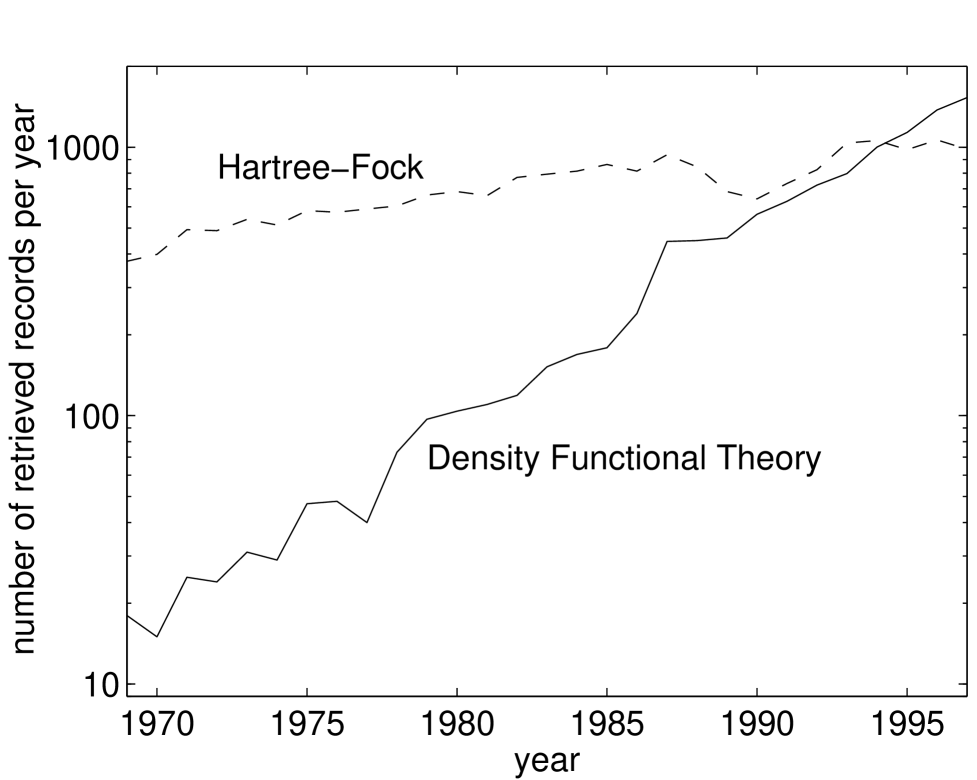
FIG. 1.: One indicator of the increasing use of DFT is the number of records retrieved from the INSPEC databases by searching for the keywords “density”, “functional” and “theory”. This is compared here with a similar search for keywords “Hartree” and “Fock”, which parallels the overall growth of the INSPEC databases (for any given year, approximately 0.3% of the records have the Hartree–Fock keywords).

This method has the double advantage of being able to treat many problems to a sufficiently high accuracy, as well as being computationally simple (simpler even than the Hartree scheme). Despite these advantages it is absent from most undergraduate and many graduate curricula with which we are familiar.

We believe that this omission stems in part from the tendency of the existing books and review papers on DFT, e.g. Refs. [1, 2, 3], to follow the historical path of development of the theory. Although appropriate for a thorough treatment, this approach unnecessarily prolongs the introduction and grapples with problems which are not directly relevant to the practitioner. It is our purpose here to give a brief and self–contained introduction to density functional theory, assuming only a first course in quantum mechanics and in thermostatistics. We break with the traditional approach by relying on the analogy with thermodynamics [4]. In this formulation, the use of the density distribution as a free variable arises in a natural manner, as do more advanced concepts which are central to recent developments in the theory [5], e.g. the exchange–correlation hole and generalized compressibilities. The discussion is sufficiently detailed to provide a useful overview for the beginning practitioner, and the relatively novel point of view may also prove illuminating for those experienced researchers who are not familiar with it. We hope that the availability of such an introduction will encourage teachers to include a one or two hour class on DFT in courses on quantum mechanics, atomic and molecular physics, condensed matter physics, and materials science.

The general theoretical framework of DFT, involving the Hohenberg–Kohn free energy $F_{\text{HK}}[n({\bf r})]$, is presented in Sec. II, which for simplicity focuses on classical systems. The generalization to the quantum–mechanical electron gas is given in Sec. III, together with the discussion of the Kohn–Sham equations and of the local density approximation, which is the simplest practical approximation for the exchange–correlation energy. Various issues relating to the accuracy of this approach are discussed in Sec. IV, followed by a summary in Sec. V.

II General theory

In this section, a unified treatment of thermodynamics and density functional theory is presented. For simplicity, the case of a classical interacting system of point particles will be discussed first. Although classical DFT has its own applications, e.g. liquids [6], the reader is advised to keep in mind electronic systems, which will be the subject of the next section. Thus, Eqs. (1) through (8), to be derived here using classical notation, are equally applicable to quantum–mechanical systems, where Hilbert space with its position and momentum operators replaces the classical phase space and its scalar coordinates.

A Thermodynamics: a reminder

We begin by rederiving the equations of thermodynamics from statistical mechanics [7]. Consider a classical system of $M$ interacting particles in a container of volume $V$. The many–body Hamiltonian is:

$${\cal H}_{\text{MB}}\;=\;{\cal T}+{\cal U}\;,$$ (1)

where ${\cal T}=\sum_{i=1}^{M}{\bf p}_{i}^{2}/2m$ is the kinetic energy, and ${\cal U}=\sum_{i<j}u(|{\bf r}_{i}-{\bf r}_{j}|)$ is the interaction energy, assuming a simple pair potential $u(r)$. Here ${\bf r}_{i}$ and ${\bf p}_{i}$ are the positions and momenta of the particles, and $m$ is their mass. We consider the grand–canonical ensemble, where the system is in contact with a heat reservoir of temperature $T$ and a particle reservoir with chemical potential $\mu$. It is well–known from statistical physics that the grand potential, which is the free energy in this case, is given by:

$$\Omega(\mu,T,V)\;=\;-T\,\log\,\Xi\;,$$ (2)

where $\Xi$ is the grand partition function,

$$\Xi(\mu,T,V)=\sum_{M=0}^{\infty}{1\over M!}{\rm Tr}\,\exp\left(-{{\cal H}_{\text{MB}}\!-\!\mu M\over T}\right)\;,$$ (3)

the temperature is in energy units (i.e. $k_{B}=1$), and the classical trace, ${\rm Tr}$, represents the $6M$–dimensional phase–space integral (the division by $M!$ compensates for double counting of many–body states of indistinguishable particles).

It follows directly from these definitions that the expectation value of the number of particles in the system is given by a derivative of the grand potential, $N=\left\langle M\right\rangle=-(\partial\Omega/\partial\mu)$. The convexity of the thermodynamic potential [8] implies that $N$ is a monotonically increasing function of $\mu$. Other partial derivatives of $\Omega$ give the values of additional physical quantities, such as the entropy, $S=-(\partial\Omega/\partial T)$ and the pressure $P=-(\partial\Omega/\partial V)$. This may be summarized by writing ${\rm d}\Omega=-N\,{\rm d}\mu-S\,{\rm d}T-P\,{\rm d}V$.

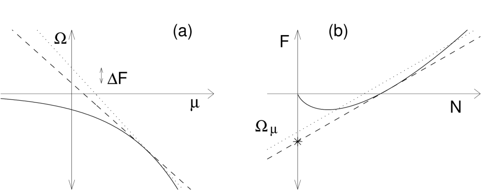
FIG. 2.: (a) The Legendre transform which gives $F(N)$ corresponds to describing the curve $\Omega(\mu)$ by the properties of its tangents: minus their slopes $N=-(\partial\Omega/\partial\mu)$ and their intercepts with the energy axis, $F=\Omega+\mu N$. The fact that the derivative $\Delta F/\Delta N$ is equal to $\mu$ follows from asking the question: if two neighboring lines intercept the energy axis at a distance $\Delta F$ from each other, and have slopes which differ by $\Delta N$, how far from the axis will they cross each other? (b) The Legendre transform back from $F(N)$ to $\Omega(\mu)$ has a similar interpretation. The minimization suggested in Eq. (4) corresponds to studying a family of lines with a fixed slope $\mu$, which pass through points $(N,F)$ on the free energy curve. Their intercepts, $\Omega_{\mu}=F-\mu N$, have a minimum (marked by an asterisk) for that line which is tangent to the curve.

A basic lesson of thermodynamics is that in different contexts it is advantageous to use different ensembles. For example, in studying systems where the number of particles rather than the chemical potential is fixed, it is preferable to use the Helmholtz free energy [9], which is obtained from the grand potential $\Omega$ by a Legendre transform: $F(N,T,V)=\Omega\left(\mu(N),T,V\vphantom{\mbox{$1\over 2$}}\right)+\mu(N)N$. Here $\mu(N)$ is no longer an independent variable, but a function of $N$ obtained by inverting the relationship $N=N(\mu,V,T)=-(\partial\Omega/\partial\mu)$. The derivative of $F$ with respect to the “new” free variable $N$ is equal to the “old” free variable $\mu$. The derivatives with respect to the other variables are unchanged (but are taken at constant $N$ rather than at constant $\mu$). We thus write ${\rm d}F=\mu\,{\rm d}N-S\,{\rm d}T-P\,{\rm d}V$.

For the purpose of comparison with DFT, it is useful to make a variation on the inverse Legendre transform which expresses $\Omega$ in terms of $F$, and to define the following “grand potential function”, which depends explicitly on both $\mu$ and $N$:

$$\Omega_{\mu}(N,T,V)\;\equiv\;F(N,T,V)-\mu N\;.$$ (4)

This function gives the original grand potential of Eq. (2) when minimized with respect to $N$, i.e. when the derivative $(\partial F/\partial N)-\mu$ vanishes, which is equivalent to the condition $N\!=\!N(\mu,T,V)$ conventionally used in the inverse Legendre transform. For other values of $N$, the function $\Omega_{\mu}(N,T,V)$ describes a “cost” in free energy of having a configuration with the “wrong” number of electrons. For a geometric interpretation of Legendre transforms, including the minimization procedure of Eq. (4), see Fig. 2.

B Nonuniform systems and the Hohenberg–Kohn theorem

The discussion above can be generalized in a quite straightforward manner to the treatment of particles in an external potential $v({\bf r})$. The many–body Hamiltonian is now

$${\cal H}_{\text{MB}}\;=\;{\cal T}+{\cal V}+{\cal U}\;,$$ (5)

where the potential energy, ${\cal V}=\sum_{i=1}^{M}v({\bf r}_{i})$, has been added. The grand potential and the partition function are defined as before, Eqs. (2) and (3), but they now depend on the potential function $v({\bf r})$ rather than on the scalar volume $V$. In this sense, $\Omega=\Omega\left(\mu,T,[v({\bf r})]\vphantom{\mbox{$1\over 2$}}\right)$ is now a functional [10] of $v({\bf r})$ as well as a function of $\mu$ and $T$ — the square brackets denote functional variables (it is also implicitly a functional of the pair potential $u(r)$). As is well known, the potential $v({\bf r})$, is an energy which is measured from an arbitrary origin, i.e. shifting the potential by a constant does not affect the physics of the system. It is convenient here to set this origin at the chemical potential, i.e. to take $\mu=0$. Equivalently, one may define the new functional variable as $v({\bf r})-\mu$, as $\Omega$ depends only on this difference, and not on $v$ and $\mu$ separately [11].

The functional derivative of $\Omega$ with respect to the new variable gives the density distribution of the particles, $n({\bf r})=\left\langle\rho({\bf r})\right\rangle=\delta\Omega/\delta v({\bf r})$, where $\rho({\bf r})=\sum_{i=1}^{M}\delta({\bf r}-{\bf r}_{i})$ is the unaveraged density. Using a (functional) Legendre transform as above, we can define a new free energy which depends on $n({\bf r})$ rather than on $v({\bf r})$, and is called the Hohenberg–Kohn free energy:

$$F_{\text{HK}}[n({\bf r})]\;=\;\Omega[v({\bf r})]\,-\int d{\bf r}\;n({\bf r})\,v({\bf r})\;,$$ (6)

where the explicit temperature variable has been omitted, and $v({\bf r})$ on the right hand side is chosen to correspond to the given $n({\bf r})$ (that such a choice is possible follows from the “generalized convexity” of the free energy [8, 12]). The partial and functional derivatives of $F_{\text{HK}}[n({\bf r})]$ are given by the usual rules for Legendre transforms: ${\mathrm{d}}F_{\text{HK}}=-S{\mathrm{d}}T-\int{\mathrm{d}}{\bf r}\>v({\bf r})\delta n({\bf r})$.

The direct generalization of the free energy function of Eq. (4) is the free energy functional:

$$\Omega_{v}[n({\bf r})]\;\equiv\;F_{\text{HK}}[n({\bf r})]\,+\int d{\bf r}\;n({\bf r})\,v({\bf r})\;,$$ (7)

with $v({\bf r})$ and $n({\bf r})$ treated as independent functional variables. If this free energy functional is minimized with respect to $n({\bf r})$ at constant $v({\bf r})$ (and given $T$, etc.), the relation

$${\frac{\delta F_{\text{HK}}}{\delta n({\bf r})}}\;=\;-v({\bf r})$$ (8)

is obtained. For $n({\bf r})$ and $v({\bf r})$ obeying this physical relation, the free energy functional is equal to the grand potential by inspection. The existence of a functional of $n({\bf r})$ with this property is one of the basic tenets of DFT, and is the (second) Hohenberg–Kohn theorem [13].

Note that below we will use Eq. (8), which also follows directly from the properties of Legendre transforms. Discussion of the Hohenberg–Kohn theorem, Eq. (7), is nevertheless important even in a Legendre–transform–based introduction to DFT, because the free–energy–minimization procedure embodied in it is central both to forming a physical intuitive picture of DFT, and to devising efficient numerical schemes for solving the DFT equations in practice [14].

C Examples

We next apply the expressions above to two (simplistic) physics problems: finding the density distribution of air and of water in the ecosphere.

1) Air: First we consider air, using the approximate model of an ideal gas. For such a gas the particles do not interact, $u(r)=0$, and the partition function can be evaluated directly. The Hamiltonian, Eq. (5), reduces to, ${\cal H}_{\text{M}B}={\cal T}+{\cal V}$. The grand partition function, $\Xi$ of Eq. (3), may be expressed as $\Xi=\sum_{M=0}^{\infty}{\Xi_{1}}^{M}/M!=\exp(\Xi_{1})$, in terms of the partition sum for a single particle, $\Xi_{1}=(2\pi\hbar)^{-3}\int{\mathrm{d}}{\bf r}{\mathrm{d}}{\bf p}\,\exp\left(-(p^{2}/2m+v)/T\vphantom{\mbox{$1\over 2$}}\right)$. The momentum integral is trivial, giving $\Xi_{1}=\int({\mathrm{d}}{\bf r}/\lambda_{T}^{3})\exp\left(-v({\bf r})/T\vphantom{\mbox{$1\over 2$}}\right)$, where volume is normalized by the “thermal wavelength” $\lambda_{T}=\sqrt{\hbar^{2}/mT}$. One finds from Eq. (2) that $\Omega=-T\Xi_{1}$. In this case the density distribution is easily found directly: $n({\bf r})=\delta\Omega/\delta v({\bf r})=\lambda_{T}^{-3}\exp\left(-v({\bf r})/T\vphantom{\mbox{$1\over 2$}}\right)$, but for pedagogical purposes we proceed to evaluate the Legendre transforms explicitly.

Inverting the ideal gas $n[v]$ relationship just derived gives $v({\bf r})=-T\log(n\lambda_{T}^{3})$, and proceeding with the functional Legendre transform of Eq. (6) gives

$$F_{\text{H}K}[n({\bf r})]=\int{\mathrm{d}}{\bf r}\;n({\bf r})\,f\left(n({\bf r}),T\vphantom{\mbox{$1\over 2$}}\right)\;,$$ (9)

where

$$f(n,T)=T\left(\log(n\lambda_{T}^{3})-1\vphantom{\mbox{$1\over 2$}}\right)\;,$$ (10)

is the free energy per particle. The latter is equal to the Helmholtz free energy per particle, $F(N,T,V)/N$, evaluated for a uniform ideal gas with $n=N/V$.

The DFT free energy functional, Eq. (7), for an ideal gas is

$$\Omega_{v}[n({\bf r})]=\int{\mathrm{d}}{\bf r}\;n({\bf r})f\left(n({\bf r}),T\vphantom{\mbox{$1\over 2$}}\right)+\int{\mathrm{d}}{\bf r}\;n({\bf r})v({\bf r})\;.$$ (11)

Minimizing this energy functional with respect to $n({\bf r})$ gives $v=-\partial(fn)/\partial n=-T\log(n\lambda_{T}^{3})$, which is equivalent to $n\propto\exp(-v/T)$, as discussed above.

The density distribution of the atmosphere in the gravitational field of the Earth may now be determined. The external potential, measured from the chemical potential, is $v({\bf r})=mgh-\mu$, where $h$ is the height and $g\simeq 10{\text{m}}/{\text{s}}^{2}$ is the acceleration due to Earth’s gravitational field (as we take $h=0$ at Earth’s surface, we have subtracted $\mu$ explicitly here). Substituting this in the expression for the density, we find that the density decreases exponentially with height, $n({\bf r})\propto\exp(-h/l)$, with a length–scale $l=T/mg$. Taking $m$ as the mass of a nitrogen molecule, $m\simeq 5\times 10^{-26}$kg, and the temperature as $T=4\times 10^{-21}$ Joules ($\simeq 17^{\circ}$C), gives $l=8\times 10^{3}$m or 8 kilometers, less than the height of the Everest (in practice, the atmosphere is not in equilibrium, $T\neq{\mathrm{c}onst.}$, and this description becomes increasingly inaccurate at higher altitudes).

2) Water: Finding the density distribution of water requires a different analysis, because the ideal gas is a good description of real fluids only for low densities such as those found in the atmosphere. At higher densities, the interactions, $u(r)$, must be taken into account. An exact, explicit evaluation of the partition function and its derivatives is no longer possible, and we are compelled to use models and approximations. The inhomogeneity of the distribution will be given an approximate treatment here, by assuming that the Hohenberg–Kohn energy may still be expressed as in Eq. (9), in terms of the Helmholtz free energy per particle for a uniform system. This is a “local density approximation”, a concept which is in common use in DFT. For simplicity, we will use the van der Waals model for $f(n,T)$. In this model [15], both attractive and repulsive interactions of real atoms and molecules (typically included in $u(r)$ for large and small $r$, respectively) are taken into account. Correspondingly, two simple modifications in the ideal–gas expressions for $f$, Eq. (10) are made: first, a “higher order in $n$” attractive term is added, and second, an “excluded volume” $b$, representing the “hard core” of real particles, is subtracted from the volume per particle $n^{-1}$ in the thermal term. The Helmholtz free–energy per particle in the uniform fluid is thus taken to be

$$f(n)=T\left(3\log(\lambda_{T})-\log(n^{-1}-b)-1\vphantom{\mbox{$1\over 2$}}\right)-an\;,$$ (12)

which replaces Eq. (10). Correspondingly, the pressure is

$$P=-\left({\partial F\over\partial V}\vphantom{\mbox{$1\over 2$}}\right)_{N}=-{\partial f\over\partial n^{-1}}={T\over n^{-1}-b}-an^{2}\;,$$ (13)

which is a more familiar expression.

The free–energy functional to be minimized with respect to $n({\bf r})$ is again that of Eq. (11), but the extremum condition,

$$v=-{\partial(nf)\over\partial n}=-T\left({b\over n^{-1}-b}+\log{\lambda_{T}^{3}\over n^{-1}-b}\vphantom{\mbox{$1\over 2$}}\right)+2an$$ (14)

may now have several solutions, and the value of $n$ which gives the lowest free energy must be selected. In the present model, for temperatures which are not too high and for a limited range of values of $v$, there are two competing local minima, corresponding to the liquid and the gas phases of the fluid [16].

We now return to water, representing a typical location on Earth as a unit of area (one square meter), covered by $10^{8}$ moles of water (one mole $\simeq 6\times 10^{23}$ molecules). We use the same potential $v=mgh-\mu$ and the same values of $T$ and $g$ as above. The mass of a water molecule is $m\simeq 18\times 10^{-3}$kg/mole, and we choose the values of $a\simeq 0.48$Pa$\times$m${}^{6}/$mole² and $b\simeq 16\times 10^{-6}$m${}^{3}/$mole to give the boiling point of water as 100 degrees Celsius at a pressure of one atmosphere $\simeq 10^{5}$Pa, and the particle density of the liquid water at that point as $n\simeq 56$moles/m³, corresponding to a mass density of $10^{3}$kg/m³. Finding the density distribution, $n(h)$, requires the inversion of Eq. (14) which is not readily available analytically; therefore we have performed this exercise numerically. The chemical potential $\mu$ plays the role of a Lagrange multiplier, imposing the constraint $\int{\mathrm{d}}{\bf r}\,n({\bf r})=N$, and finding it requires a few trials or iterations (using the Newton–Raphson algorithm).

The resulting value of $\mu$ is $-2.5385\times 10^{5}$ Joules/mole — several significant digits must be kept because $v$ (or $v-\mu$) varies by only 180 Joules/mole for each kilometer of altitude. The density distribution $n({\bf r})$ contains both liquid and gaseous regions. The liquid region or “ocean” occupies the lower altitudes, and a gaseous region occupies higher altitudes. In the lower region, the fluid is more or less incompressible, with the density at $h=0$ higher by only a couple of percent than that at “sea level”, $h\simeq 1750$m. Above this point one finds water vapor with a density of $\simeq 4$moles/m³, corresponding to a pressure of $10^{4}$Pa or one–tenth of an atmosphere (real water deviates significantly from our van der Waals model — a more accurate description of $f(n)$ would give $\sim 2.5\times 10^{3}$Pa). At this low density, the equation of state of the water vapor does not differ significantly from that of an ideal gas, and indeed one finds an exponential decay with further increase in altitude, as discussed above for air (the lengthscale in this case is $\simeq 14$km, as the water molecules are lighter).

Obviously, water and air coexist on the surface of Earth, and taking this into account would modify the results of our examples (most importantly, the atmosphere begins only at sea level). Such situations can be addressed by generalizing the free–energy density, $nf$, allowing it to depend on both densities $n_{\text{water}}$ and $n_{\text{air}}$. With a sufficiently accurate parameterization of $f$, a good description of many nonuniform thermodynamic systems can thus be obtained. However, for such a local description to hold, the spatial variations in $n({\bf r})$ (or equivalently, in $v({\bf r})$) must be very slow on the scale of the range of the potential $u({\bf r})$. In contrast, one may be interested in studying how the density distribution $n({\bf r})$ near a liquid–vapor interface changes gradually, on a scale of Angstroms, from that of the liquid to that of the gas. Such problems are typical applications of the DFT of classical systems, and must employ nonlocal model functionals

A discussion of such nonlocal classical functionals is beyond the scope of the present paper, but we would like nevertheless to mention the following two points: (a) As opposed to gases, classical liquids and solids are characterized by strong and complicated correlations between particles, even when the interaction potential $u(r)$ is simple. This makes the task of finding good $F_{\mathrm{H}K}[n]$ functionals nontrivial. (b) The general framework of DFT can nevertheless give accurate descriptions of real systems, provided that one uses good “anchoring points”. For example, the hard–sphere liquid has been studied extensively numerically, and accurate information for it is available. A good description of the liquid–solid transition in several more general systems may be found by perturbing in the difference between the actual $u(r)$ and that of the hard sphere system, $u_{\text{hs}}(r)$, e.g. by taking $F_{\mathrm{H}K}[n]=F_{\text{hs}}+\int{\mathrm{d}}r\>(u-u_{\text{hs}})\left(\delta F_{\mathrm{H}K}/\delta u(r)\vphantom{\mbox{$1\over 2$}}\right)$, where in the last term, the functional derivative is equal to $\delta\Omega/\delta u(r)$ which is the pair correlation function. With this as background, we now proceed to treat electronic systems in the next section.

III Application to electrons

The electron is much lighter than an atom or molecule, and thus has a relatively large thermal wavelength, e.g. $\lambda_{T}\simeq\hbar/\sqrt{mT}\simeq 17$Å at room temperature, more than an order of magnitude larger than the typical inter–electron distance. Its treatment must be quantum–mechanical, with the Hamiltonian of Eq. (5) replaced by the corresponding operator, $\hat{H}_{\text{MB}}=\hat{T}+\hat{V}+\hat{U}$. The statistical–mechanics derivation above is affected by this, e.g. the trace (Tr) in the definition of the partition function, Eq. (3), is taken over the Hilbert space rather than over the classical phase space. However, the thermodynamic considerations and Legendre transforms, including Eqs. (6), (7) and (8) for nonuniform systems, are unchanged.

As electrons are Fermions, they form a degenerate gas at the prevailing high densities, and their energy in the cases of interest here does not deviate considerably from its ground–state value. Indeed, electronic DFT was developed in Refs. [13] and [17] as a ground–state theory. Correspondingly, we will from here on take the zero temperature limit, $T\to 0$, in all our equations and expressions (cf. Ref. [18]). In this limit the partition function is dominated by a single quantum–mechanical state with an integer number of electrons, $M=N$, and the grand potential is equal to the ground–state energy (using our $\mu=0$ convention). The Hohenberg–Kohn free–energy, $F_{\text{HK}}[n]$, is then, by Eq. (6), equal to the total energy minus the potential energy, i.e. to the internal energy.

For noninteracting quantum mechanical particles, $u(r)=0$, the internal energy is just the kinetic energy, for which we introduce the notation $F_{\text{ni}}[n]=F_{\text{HK}}[n]\left.\vphantom{A\over B}\right|_{u(r)=0}$. Whereas in the classical case, the noninteracting or ideal–gas system had simple local expressions for the energy functionals, here the relationships between the energy, the density distribution, and the confinement potential are nontrivial and nonlocal.

Practical implementations of DFT require an explicit construction of the Hohenberg–Kohn free–energy functional, $F_{\text{HK}}[n]$. It is customary to write $F_{\text{HK}}[n]$ for interacting electrons as a sum of the noninteracting kinetic energy, $F_{\text{ni}}[n]$, and two interaction terms — the electrostatic energy and the exchange–correlation energy [19]:

$$F_{\text{HK}}[n({\bf r})]\;=\;F_{\text{ni}}[n({\bf r})]+E_{\text{es}}[n({\bf r})]+E_{\text{xc}}[n({\bf r})]\;,$$ (15)

where the last term, $E_{\text{xc}}[n]$, is defined as the remainder and thus contains everything that is not included in the first two terms. Each of the three terms on the right hand side is in principle a functional of the independent variable $n({\bf r})$. Only the second term — the electrostatic energy — is easily expressed explicitly:

$$E_{\text{es}}[n({\bf r})]\;=\;{\frac{e^{2}}{2}}\int{d{\bf r}\,d{\bf r}^{\prime}\over|{\bf r}\!-\!{\bf r}^{\prime}|}\>n({\bf r})\,n({\bf r}^{\prime})\;,$$ (16)

The first and last terms are much more complicated: knowledge of the former implies a full understanding of the quantum–mechanical noninteracting problem; the latter contains all of the many–body physics, and is in principle even more complex.

In the following, we briefly introduce two alternative methods for confronting this situation: (i) construction of explicit approximate expressions for both $F_{\text{ni}}[n]$ and $E_{\text{xc}}[n]$, and (ii) the orbital method developed by Kohn and Sham, which uses the noninteracting Schrodinger equation to evaluate $F_{\text{ni}}[n]$, with only the smaller term, $E_{\text{xc}}[n]$, replaced by explicit approximations to the desired complicated functional.

A Explicit functionals

One of the simplest models of the electronic structure of atoms was developed by Thomas [20] and Fermi [21] already in the late 1920’s. For the noninteracting part of the calculation, they used a local density approximation:

$$F_{\text{ni}}[n({\bf r})]\simeq C\int n^{5/3}({\bf r})\>d{\bf r}\;,$$ (17)

with $C={\frac{3}{10}}(3\pi^{2})^{2/3}\simeq 2.87$ in atomic units; here $Cn^{5/3}({\bf r})$ is the kinetic energy density of a uniform electron–gas of density $n({\bf r})$. They also approximated the Coulomb interaction energy of the electrons by the electrostatic term only, which corresponds in the present language to taking $E_{\text{xc}}[n]=0$. Using these simplifications and the spherical symmetry of an atom, analytical progress could be made.

Both approximations made in the Thomas–Fermi model are expected to be accurate at very high densities. The approximation made for the noninteracting part is accurate when the density of electrons changes slowly in space relative to the Fermi wavelength, or equivalently, if the density is sufficiently high that $n({\bf r})^{1/3}$ is (much) larger than the spatial rate of change of the density. The approximate treatment of the interactions, which ignores exchange and correlation effects, is the leading order of a high–density expansion, in powers of $r_{\text{s}}/a_{0}$ where $r_{s}=(3/4\pi n)^{-1/3}$ is the Wigner–Seitz radius, and $a_{0}=\hbar^{2}/me^{2}=0.53$Å is the Bohr radius. The Thomas–Fermi model indeed has applications for very dense matter, and is useful in the description of certain stars [22]. Unfortunately, the results for more down–to–earth systems are rather poor. For example, it is known that in the Thomas–Fermi model no molecules can form — the dissociated atoms always have a lower energy [23].

The Thomas–Fermi method was extended over the years in two main directions. At first, approximate expressions for the exchange–correlation energy were included, but this did not lead to significant improvements in the results. Such improvements were obtained only when an element of nonlocality was taken into account in the noninteracting kinetic energy term, $F_{\text{ni}}[n]$. This was achieved by including gradient terms (e.g. terms proportional to $|\nabla n|^{2}$ in the integrand of Eq. (17), with $n$–dependent prefactors), and lead in particular to the possibility of modeling chemical bonds. However, the description of electronic structure by the Thomas–Fermi model and its extensions remains qualitative to date [24].

B The Kohn–Sham equations

In 1965, Kohn and Sham [17] made a major step towards quantitative modeling of electronic structure, by introducing an orbital method by which $F_{\text{ni}}[n]$ can be evaluated exactly. In other words, in order to evaluate the kinetic energy of $N$ noninteracting particles given only their density distribution $n({\bf r})$, they simply found the corresponding potential, called $v_{\text{eff}}({\bf r})$, and used the Schrodinger equation,

$$\left(-{\frac{\hbar^{2}}{2m}}\nabla^{2}+v_{\text{eff}}({\bf r})\vphantom{\mbox{$1\over 2$}}\right)\psi_{i}({\bf r})=\epsilon_{i}\psi_{i}({\bf r})\;,$$ (18)

such that $n({\bf r})=\sum_{i=1}^{N}|\psi_{i}({\bf r})|^{2}$. The states $\psi_{i}$ here are ordered so that the energies $\epsilon_{i}$ are non–decreasing, and the spin index is included in $i$. If $\epsilon_{N}$ is degenerate with $\epsilon_{N+1}$ (and also at finite temperatures [25]), fractional occupations $f_{i}$ are to be used, $n({\bf r})=\sum_{i=1}^{\infty}f_{i}|\psi_{i}({\bf r})|^{2}$, but if only spin–degeneracy is involved, the result for the density is not affected. The kinetic energy is then given by $F_{\text{ni}}[n({\bf r})]=\sum_{i=1}^{N}\langle\psi_{i}|\hat{t}_{i}|\psi_{i}\rangle=\sum_{i=1}^{N}\epsilon_{i}-\int{\mathrm{d}}{\bf r}\,n({\bf r})v_{\text{eff}}({\bf r})$, where $\hat{t}_{i}$ is the kinetic energy operator for the $i$th electron ($\hat{T}=\sum_{i}\hat{t}_{i}$).

In practice, it is the external potential of a given system which is known, not the density distribution or the effective potential. One may find the effective potential by taking a functional derivative of the three–term expression for $F_{\text{H}K}[n]$, Eq. (15), and rearranging the terms:

$$v_{\text{eff}}({\bf r})=v({\bf r})-e\varphi({\bf r})+v_{\text{xc}}({\bf r})\;,$$ (19)

where we have used Eq. (8), $\delta F[n]/\delta n=-v$, for both the interacting and the noninteracting system. The electrostatic potential is here

$$\varphi({\bf r})\;=\;-e\int d{\bf r}^{\prime}\>{\frac{n({\bf r}^{\prime})}{|{\bf r}\!-\!{\bf r}^{\prime}|}}\;,$$ (20)

and the exchange–correlation potential is defined as

$$v_{\text{xc}}({\bf r})\;=\;{\frac{\delta E_{\text{xc}}}{\delta n({\bf r})}}\;.$$ (21)

Given a practical approximation for $E_{\text{xc}}[n]$, one obtains $v_{\text{xc}}({\bf r})$, and can thus find $v_{\text{eff}}({\bf r})$ from $n({\bf r})$ for a given $v({\bf r})$.

The set of equations described above is called the Kohn–Sham equations of DFT, and must be solved self–consistently: $v_{\text{eff}}({\bf r})$ determines $n({\bf r})$ in Eq. (18), and is determined by it in Eq. (19). They provide a mechanism for minimizing the functional $E_{v}[n]$ (or $\Omega_{v}[n]$) of Eq. (7), despite the fact that $F_{\text{ni}}[n]$ is known only implicitly. This method assumes that the external potential $v({\bf r})$ and the total number of electrons $N$ are given, and does not use the chemical potential $\mu$ (if a nonzero value of $\mu$ were restored, it would simply shift both sides of Eq. (19) by a constant, and thus drop out of consideration). Together with any explicit approximation for the exchange–correlation term (see below), it provides an efficient scheme for finding $n({\bf r})$ and the ground state energy [26] for a system of $N$ interacting particles. Note that for the interacting system, only the energy and its derivatives (including $n({\bf r})$) are accessible — the complicated many–body wavefunctions do not take part in this scheme.

Historically, additional properties [27] of the Kohn–Sham noninteracting system, e.g. the band structure for crystals, have also provided surprisingly accurate predictions when compared with experiments. In fact, the agreement between the calculated Kohn–Sham Fermi surface and the measured one was so remarkable for some systems [28], that it motivated analyses of soluble (perturbative) models for which the difference between the interacting and noninteracting Fermi surfaces could be calculated explicitly, and shown not to vanish [29]. Clearly, the accuracy of DFT predictions for ground–state energies and density distributions can be improved by finding better practical approximations for $E_{\text{xc}}[n]$, whereas improving the accuracy of such band–structure calculations may require “going back to the drawing board” and devising other, more appropriate, calculational schemes [30].

C The Local Density Approximation

As a practical approximate expression for $E_{\text{xc}}[n]$, Kohn and Sham [17] suggested what is known in the context of DFT as the local density approximation, or LDA:

$$E_{\text{xc}}[n({\bf r})]\;\simeq\;\int d{\bf r}\;n({\bf r})\>\epsilon_{\text{xc}}(n({\bf r}))\;,$$ (22)

where $\epsilon_{\text{xc}}(n)$ is the exchange–correlation energy per electron in a uniform electron gas of density $n$. This quantity is known exactly in the limit of high density, and can be computed accurately at densities of interest, using Monte Carlo techniques (i.e. there are no free parameters). In practice one usually employs parametric formulas, which are fitted to the data and are accurate to within 1–2%. As an example, we quote that given by Gunnarson and Lundqvist (Ref. [31]): $\epsilon_{\text{xc}}(n)=-0.458/r_{s}-0.0666G(r_{s}/11.4)$ Hartrees, where $r_{\text{s}}$ is in units of the Bohr radius, and $G(x)={\frac{1}{2}}\{(1\!+\!x^{3})\log(1\!+\!x^{-1})-x^{2}+{\frac{1}{2}}x-{\frac{1}{3}}\}$, see Fig. 3.

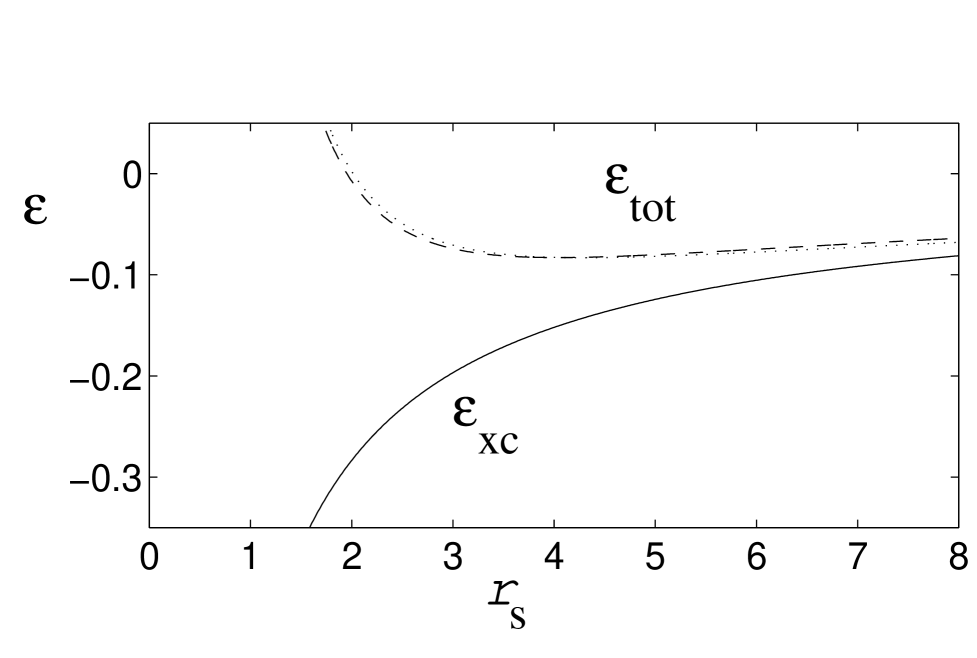
FIG. 3.: The exchange–correlation energy per electron, $\epsilon_{\text{xc}}(n)$ (in Hartrees) of a uniform electron gas, as a function of the density, parameterized by the Wigner–Seitz radius (in Bohr radii), according to the interpolation formula of Ref. [31]. The dashed line is the corresponding total energy per electron, i.e. includes the kinetic energy. The Monte–Carlo data, if plotted, would be indistinguishable on the scale used here from the curves shown. For reference, we also show the total energy per electron (dotted line) according to an alternative parameterisation, the well–known Wigner interpolation formula, Ref. [32].

Note that the only difference between the resulting computational scheme and a naive mean–field approach is the addition of the potential

$$v_{\text{xc}}({\bf r})\;=\;\left.{d\,\left(n\,\epsilon_{\text{xc}}(n)\vphantom{\mbox{$1\over 2$}}\right)\over dn}\right|_{n=n({\bf r})}$$ (23)

to the electrostatic potential at the appropriate step in the self–consistency loop [33]. The corresponding expression for the ground–state energy is:

$$E_{0}=\sum_{i=1}^{N}\epsilon_{i}-E_{\text{es}}[n({\bf r})]+\int d{\bf r}\;n({\bf r})\,\left(\epsilon_{\text{xc}}(n({\bf r}))-v_{\text{xc}}(n({\bf r}))\vphantom{\mbox{$1\over 2$}}\right)\;,$$ (24)

where the first term is the noninteracting energy, the second term subtracts half of the double counting of the electrostatic energy as in the Hartree scheme, and the last term is a similar subtraction for the exchange–correlation energy.

The LDA has been shown to give very good results for many atomic, molecular and crystalline interacting electron systems, even though in these systems the density of electrons is not slowly varying. As an example, we show in Fig. 4

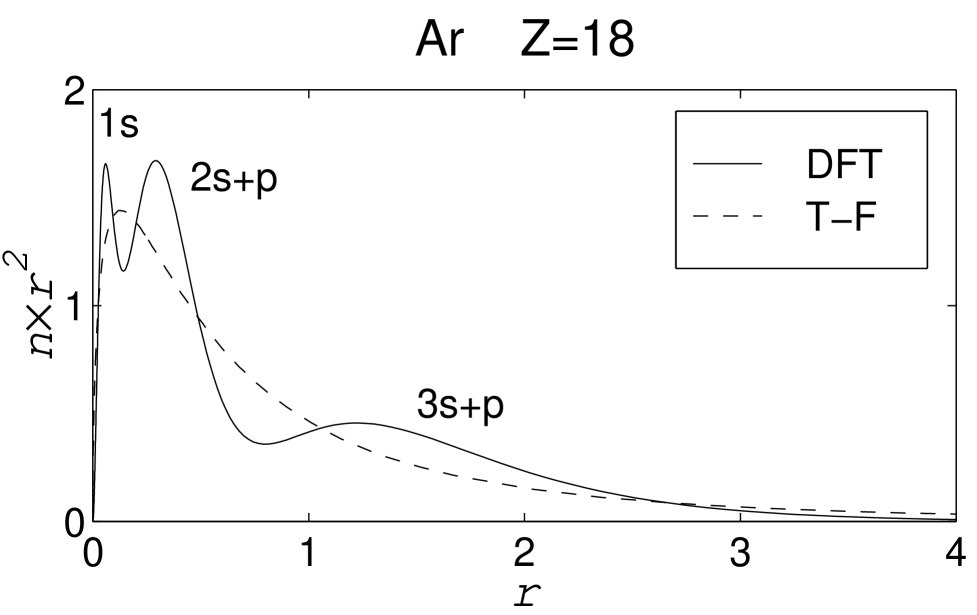
FIG. 4.: The density $n(r)$ for an Argon atom, multiplied by $r^{2}$ for convenience of presentation (inverse Bohr radii), as a function of the distance from the origin (in Bohr radii). The full line is the DFT result using the LDA, and shows the shell structure; the dashed line is the result of the Thomas–Fermi model for this atom.

the solution for an atom of Argon. One can see that the shell structure, which is absent in the Thomas–Fermi model, is described here in detail. The calculated ground–state energy is $-525.9$ Hartrees, compared to $-652.7$ Hartrees in the Thomas–Fermi model (one Hartree $=me^{4}/\hbar^{2}=27.2$eV). The experimental value is $-527.6$ Hartrees — the LDA result is accurate to within less than half a percent, compared to the 20% inaccuracy of the Thomas–Fermi model. Both the description of the shell structure and much of the improvement in the energy estimate are due to the introduction by Kohn and Sham of an exact method for evaluating the highly nonlocal kinetic energy functional. However, the accuracy of the exchange–correlation term is also of central importance, and will be discussed next.

IV Accuracy of the exchange–correlation energy

In this section, we discuss a few aspects of $E_{\text{xc}}[n]$ which are somewhat more advanced (and may be skipped in a first reading). In the first subsection, a formally exact expression for the exchange–correlation energy is derived, and a sum–rule which applies to it is obtained. The next subsection provides references to some more recent and accurate approximations, which were devised with this sum–rule in mind. Finally, a general discussion of the level of accuracy achieved by these approximations for different applications is given.

A The exchange–correlation hole

A deeper understanding of the exchange–correlation energy can be achieved by considering a continuous transition between the interacting and noninteracting systems which appear in the definition of $E_{\text{xc}}[n]$, rather than using a simple subtraction as in Eq. (15). To do this, we reduce the strength of the Coulomb interaction, $e^{2}$, and contemplate a more general interaction potential, $u(r)=\Lambda e^{2}/r$ with $0\leq\Lambda\leq 1$. In other words, we define the Hamiltonian as ${\hat{H}}_{\text{M}B}={\hat{T}}+{\hat{V}}+\Lambda{\hat{U}}$, with the noninteracting system corresponding to $\Lambda=0$, and the interacting–electron system to $\Lambda=1$. For a given density distribution $n({\bf r})$ one can consider $F_{\text{HK}}[n]$ for intermediate values of $\Lambda$, which leads to the exact expression [34]:

$$F_{\text{HK}}[n]\;=\;F_{\text{ni}}[n]+\int_{0}^{1}{\frac{\partial F_{\text{HK}}[n]}{\partial\Lambda}}\>d\Lambda\;.$$ (25)

The general rules for Legendre transforms give the derivative $\partial F_{\text{HK}}[n]/\partial\Lambda$ as equal to ${\partial\Omega/\partial\Lambda}$, which in turn is equal to $\left\langle\hat{U}\right\rangle$, the expectation value of the interaction energy ${\hat{U}}$. Note that the derivative of $\Omega$ is taken at a constant potential, but in order to reproduce the given density distribution $n({\bf r})$, this potential must depend on $\Lambda$ (it is usually denoted by $v_{\Lambda}({\bf r})$, but we need it here only at the two extremes, for which we already have appropriate notations: $v_{1}({\bf r})=v({\bf r})$ and $v_{0}({\bf r})=v_{\text{eff}}({\bf r})$).

Comparing Eq. (25) with Eq. (15), we find that $E_{\text{xc}}[n]=\int_{0}^{1}{\mathrm{d}}\Lambda\,\left\langle\hat{U}\right\rangle-E_{\text{es}}[n]$, i.e. the exchange–correlation energy is the difference between the $\Lambda$–averaged expectation value of the interaction energy and the electrostatic approximation to it. Both of these are integrals over the product of the Coulomb interaction and the density of pairs, which is $\mbox{$1\over 2$}\left\langle\hat{\rho}({\bf r})\left(\hat{\rho}({\bf r}^{\prime})-\delta({\bf r}-{\bf r}^{\prime})\vphantom{\mbox{$1\over 2$}}\right)\right\rangle$ and $\mbox{$1\over 2$}n({\bf r})n({\bf r}^{\prime})$ for the exact and approximate expressions, respectively (the factor of $1\over 2$ corrects for the double counting of each pair, and the $\delta$ function removes the interaction of each electron with itself). We are thus motivated to define a pair correlation function, $g({\bf r},{\bf r}^{\prime})$, equal to the difference between the two pair densities

$$g({\bf r},{\bf r}^{\prime})\;=\;\left\langle\hat{\rho}({\bf r})\left(\hat{\rho}({\bf r}^{\prime})-\delta({\bf r}-{\bf r}^{\prime})\vphantom{\mbox{$1\over 2$}}\right)\right\rangle_{n({\bf r}),\Lambda}-\>n({\bf r})\,n({\bf r}^{\prime})\;.$$ (26)

It is of relevance here that $g({\bf r},{\bf r}^{\prime})$ at typical electron densities is relatively featureless — it is only at very low densities ($r_{\text{s}}\sim 100a_{0}$) that electrons tend to develop strong correlations, and may form a Wigner crystal.

Using the fact that the number of particles, $M=\int{\mathrm{d}}{\bf r}^{\prime}\,\hat{\rho}({\bf r}^{\prime})$, does not fluctuate at very small temperatures, and is equal to its expectation value, $N=\int{\mathrm{d}}{\bf r}^{\prime}\,n({\bf r}^{\prime})$, it is easy to show that $\int{\mathrm{d}}{\bf r}^{\prime}\>g({\bf r},{\bf r}^{\prime})=-n({\bf r})$. It is convenient to define a normalized version of this correlation function $\rho_{\text{xc}}({\bf r},{\bf r}^{\prime};[n],\Lambda)=g({\bf r},{\bf r}^{\prime})/n({\bf r})$, which is the density of the so–called exchange–correlation hole. $\rho_{\text{xc}}$ describes the region in ${\bf r}^{\prime}$–space from which an electron is “missing” if it is known to be at the point ${\bf r}$, and the fact that its integral over ${\bf r}^{\prime}$ is equal to $-1$ corresponds to the fact that there is exactly one “missing” electron. In terms of the $\Lambda$–integrated value of this quantity,

$$w({\bf r},{\bf r}^{\prime})=\int_{0}^{1}{\mathrm{d}}\Lambda\;\rho_{\text{xc}}({\bf r},{\bf r}^{\prime};[n],\Lambda)=\int_{0}^{1}{\mathrm{d}}\Lambda\;g({\bf r},{\bf r}^{\prime})/n({\bf r})\;,$$ (27)

the exchange–correlation energy is given formally as

$$E_{\text{xc}}[n({\bf r})]\;=\;{\frac{e^{2}}{2}}\int{\frac{d{\bf r}\,d{\bf r}^{\prime}}{|{\bf r}\!-\!{\bf r}^{\prime}|}}\>n({\bf r})\>w({\bf r},{\bf r}^{\prime})\;.$$ (28)

In other words, the exact exchange–correlation energy may be written as in the LDA, Eq. (22), provided that the corresponding energy per particle, $\epsilon_{\text{xc}}$ is interpreted not as a local quantity but is evaluated according to the density of the exchange–correlation hole, $\epsilon_{\text{xc}}=(e^{2}/2)\int{\mathrm{d}}{\bf r}^{\prime}\,w({\bf r},{\bf r}^{\prime})/|{\bf r}-{\bf r}^{\prime}|$.

The normalization property of the exchange–correlation hole, $\rho_{\text{xc}}$, carries over to its $\Lambda$–averaged counterpart:

$$\int{\mathrm{d}}{\bf r}^{\prime}\;w({\bf r},{\bf r}^{\prime})=-1\;.$$ (29)

This “sum–rule”, Eq. (29), has been used [35] as the basis for an “explanation” of the relatively high accuracy achieved by the LDA: the reference system here (the homogeneous electron gas) has properties which are also exact for the inhomogeneous system. More importantly, it restricts and guides the search for more accurate practical approximations: expressions which break the sum–rule can not be expected to work well (see below).

B Refinements of $E_{\text{xc}}$

The fact that the LDA achieves a high relative accuracy, i.e. can predict the ground–state energy of various systems to within less than a percent, does not mean that the absolute accuracy is sufficient. In particular, typical applications in chemistry require that the energy of a molecule be known to within a small fraction of an electron–volt. Indeed, improving upon the accuracy of the LDA is a goal which has been persistently pursued. One improvement which is very often implemented is the local spin–density (LSD) approximation [36], which is motivated in part by the fact that the exchange–correlation hole is very different for electrons with parallel and with antiparallel spins. In this scheme, separate densities of spin–up and spin–down electrons are used as a pair of functional variables: $n_{\uparrow}({\bf r})$ and $n_{\downarrow}({\bf r})$, and the Hamiltonian contains separate potentials for spin up and spin down electrons — a Zeeman–energy magnetic field term is introduced. The exchange–correlation energy per particle is then taken from the results for a homogeneous spin–polarized electron gas, $\epsilon_{\text{xc}}(n_{\uparrow},n_{\downarrow})$. The spin dependence allows Hund’s rule to be discussed within DFT.

The next degree of sophistication is to allow $\epsilon_{\text{xc}}$ to depend not only on the local densities but also on the rate–of–change of the densities, i.e. to add gradient corrections. Unfortunately, it was found that such corrections do not necessarily improve the accuracy obtained. In fact, introducing gradient corrections in a straightforward and systematic manner, by expanding around the uniform electron gas, breaks the sum rule of Eq. (29) and is less accurate [35]. This situation led to the development of various generalized gradient approximations (GGAs) [37, 38], in which the spatial variations of $n({\bf r})$ enter in a manner which conforms with the sum rule, and which have succeeded in reducing the errors of the LDA by a factor which is typically about 4.

Further improvements in practical expressions for $E_{\text{xc}}[n]$ are actively being pursued [39]. One direction which may perhaps achieve the accuracy needed for applications in chemistry [40], is to use the fact that the exact form of the exchange–correlation hole can be calculated for $\Lambda=0$ relatively easily, directly from the noninteracting Kohn–Sham system. There is thus no need to use an approximation such as the LDA or the GGA for the low–$\Lambda$ portion of the integral in Eq. (28). Ultimately, one hopes that a systematic method of improving the approximation would be found, although so far this has been an elusive goal.

C Successes and failures

Over the years, many different types of applications of DFT have been developed. This variety evolved because knowledge of the electronic ground–state energy as a function of the position of the atomic nuclei determines molecular and crystal structure, and gives the forces acting on the atomic nuclei when they are not at their equilibrium positions. At present, DFT is being used routinely to solve problems in atomic and molecular physics, such as the calculation of ionization potentials [41] and vibration spectra, the study of chemical reactions, the structure of bio–molecules [42], and the nature of active sites in catalysts [43], as well as problems in condensed matter physics, such as lattice structures [44], phase transitions in solids [45], and liquid metals [46]. Furthermore these methods have made possible the development of accurate molecular dynamics schemes in which the forces are evaluated quantum mechanically “on the fly” [47].

It is important to stress that all practical applications of DFT rest on essentially uncontrolled approximations, such as the LDA discussed above. Thus the validity of the method is in practice established by its ability to reproduce experimental results. A discussion of the accuracy achieved by DFT, compared to other alternative approaches, necessarily depends very much on the specific applications one has in mind, as detailed below.

For atoms and small molecules, the simplest version of the LDA already provides a very useful qualitative and semi–quantitative picture. It is of course a dramatic improvement over the Thomas–Fermi model. It even improves on the more labor–intensive Hartree–Fock method in many cases, especially when one is calculating the strength of molecular bonds, which are substantially overestimated in Hartree–Fock calculations. This can only be considered as a surprising success, keeping in mind that an isolated atom or molecule is as inhomogeneous an electronic system as possible, and therefore the last place where one might expect a local approximation to work. In other words, electronic correlations in such systems are in a sense weak, and are on average similar to those of a uniform electron gas (see the discussion of the sum–rule, Eq. (29)). However, the many–body quantum states of such relatively small systems can be solved for extremely accurately using well–known techniques of quantum chemistry, specifically the configuration interaction (CI) method [48]. Furthermore, these techniques use controlled approximations, so that the accuracy can be improved indefinitely, given a powerful enough computer, and indeed impressive agreement with experiment is routinely achieved. For this reason, most quantum chemists did not embrace DFT at an early stage.

It is in studies of larger molecules that DFT becomes an indispensable tool [5]. The computational effort required in the conventional quantum chemistry approaches grows exponentially with the number of electrons involved, whereas in DFT it grows roughly as the third power of this number. In practice, this means that DFT can be applied to molecules with hundreds of atoms, whereas using CI, one is limited to systems with only a few atoms. Simply solving the noninteracting problem for a complicated molecule may also be prohibitive, and various methods are used in order to reduce the problem to a computationally manageable task. Of these, we mention the well–known pseudopotential method [14], which allows one to avoid recalculating the wavefunctions of the inert core electrons over and over again, and the recent attempts to develop “order N” methods [49], which make use of the fact that the behavior of the densities at each point is determined primarily by the atoms in its immediate vicinity, rather than by the whole molecule. It is for this problem that more and more accurate density functionals are most obviously needed. To illustrate this, we quote one sentence from Ref. [38]: “Accurate atomization energies are found [using the GGA] for seven hydrocarbon molecules, with a rms error per bond of 0.1 eV, compared with 0.7 eV for the LSD approximation and 2.4 eV for the Hartree–Fock approximation.”

The remarkable usefulness of DFT for solid–state physics was apparent from the outset. For example, the lattice constants of simple crystals are obtained with an accuracy of about 1% already in the LDA [50]. In such applications, the electronic structure of a single unit cell with periodic boundary conditions is studied; more ambitious applications are also common, e.g. a supercell containing many unit cells with a single impurity or defect [51]. Admittedly, this method is inappropriate for treating some more complicated situations, such as antiferromagnets or systems with strong electronic correlations. In other cases, such as for the work–function of metals, local approximations such as the LDA obviously miss an important part of the physics: for a point ${\bf r}$ a short distance away from the surface of a metal, the exchange–correlation hole $\rho_{\text{xc}}({\bf r},{\bf r}^{\prime})$ is concentrated at points ${\bf r}^{\prime}$ inside or very near the surface of the metal; this results in image forces, i.e. a $1/r$ behavior of $v_{\text{xc}}$ (where $r$ is the distance from the surface) which is nonlocal. However, this deficiency can be corrected for “by hand”, yielding satisfactory results [52].

In general it is useful to note that, in contrast to approximations using free parameters which are empirically optimized to fit a certain set of data and may thus be used reliably for interpolation, the LDA and the GGA have proved to exhibit a consistent degree of accuracy or inaccuracy for a wide variety of problems — when applied to a new problem, the results can thus be interpreted with some confidence. One should of course also be aware of the cases for which these approximations are known to fail, such as the image forces mentioned above, and van der Waals forces [53], which are important e.g. for biological molecules. Both of these are manifestations of the significance of nonlocal correlations — a nonlocality which is by definition absent from the LDA and its immediate extensions. These examples of practical failure, together with the unattractiveness of uncontrolled approximations, spur research towards new and more exact exchange–correlation energy functionals.

Our discussion would not be complete without mentioning the existence of many other uses of density–functional methods, for electronic systems and for other physical systems. The former include time–dependent DFT, which relates interacting and noninteracting electronic systems moving in time–dependent potentials, and relativistic DFT, which uses the Dirac equation rather than the Schrodinger equation to calculate the Kohn–Sham states (these are reviewed in Ref. [2]). The latter include applications in nuclear physics, in which the densities of protons and neutrons and the resulting energies are studied [54], and in the theory of liquids, as already discussed in Sec. II.

V Summary

In describing density functional theory (DFT) and the approximations typically implied by its use, it is necessary to follow two steps, as was done in considerable detail in Secs. II and III above. The first step is to introduce the Hohenberg–Kohn energy, $F_{\text{HK}}[n({\bf r})]$. It is equal to the internal energy, i.e. the difference between the ground–state energy $E_{0}$ and the potential energy, or the sum of the kinetic energy and the interaction energy of the electrons. $F_{\text{HK}}[n]$ is a universal functional of the density distribution — it applies to atoms, molecules, crystals, and all other electronic systems. The existence of $F_{\text{HK}}[n]$ arises from the fact that each system has not only a unique external potential, $v({\bf r})$, as in traditional many–body theory, but also a unique density distribution, $n({\bf r})$. Within DFT, the different systems are labeled by their different electronic densities, $n({\bf r})$, and the potential $v({\bf r})$ is considered as secondary to, and dependent on, the primary $n({\bf r})$. In fact, the potential is given by the functional derivative $v({\bf r})=-\delta F_{\text{HK}}/\delta n({\bf r})$. This property of $F_{\text{HK}}[n]$ can be deduced in two equivalent ways: (a) it is the Euler equation for the Hohenberg–Kohn theorem, which is a variational principle stating that the total energy, $F_{\text{HK}}[n]+\int{\mathrm{d}}{\bf r}\>n({\bf r})v({\bf r})$, is minimized for a given $v({\bf r})$ by the corresponding ground–state density $n({\bf r})$, and has the ground–state energy $E_{0}$ as its minimum value; (b) it arises as the conjugate of the well–known relationship $n({\bf r})=\delta E_{0}/\delta v({\bf r})$, when the definition $F_{\text{HK}}[n]=E_{0}-\int{\mathrm{d}}{\bf r}\>n({\bf r})v({\bf r})$ is viewed as a (functional) Legendre transform.

The functional $F_{\text{HK}}[n({\bf r})]$ discussed above is not known explicitly in terms of its variable, $n({\bf r})$. The second crucial step is to introduce a practical approximation for this energy functional. It may be written as a sum of three terms: (i) the kinetic energy term, which is by definition equal to the value $F_{\text{HK}}[n({\bf r})]$ would have for noninteracting electrons; (ii) the Hartree term, which is simply a double integral over $n({\bf r})n({\bf r}^{\prime})$; and (iii) the remainder or exchange–correlation term, which in principle contains all of the complicated interaction physics ignored by the first two terms, and must be approximated in practice. By taking a functional derivative, one finds that the external potential $v({\bf r})$ is given by a corresponding sum of three terms: (i) the so–called effective potential, $v_{\text{eff}}({\bf r})$, which is the potential which a system of noninteracting electrons must have in order to reproduce the $n({\bf r})$ of the interacting system, (ii) the electrostatic potential, and (iii) an exchange–correlation potential. The simplest widely–used expression for the exchange–correlation term is the local density approximation (LDA), which takes the exchange–correlation energy–density at each point in the system to be equal to its known value for a uniform interacting electron gas of the same density, and results in a parameter–free approximate description of all electronic systems.

These ideas are implemented by the Kohn–Sham set of equations, which consists of a noninteracting Schrodinger equation involving the effective potential $v_{\text{eff}}({\bf r})$, the abovementioned relationship between $v_{\text{eff}}({\bf r})$ and the given external potential $v({\bf r})$, and expressions for the density distribution $n({\bf r})$ and the interacting ground–state energy $E_{0}$ in terms of the properties of the noninteracting single–particle solutions and of the approximate expression for the exchange–correlation energy which is in use. Using modern computers, the Kohn–Sham equations can be solved even for systems containing dozens of atoms, and the results for the ground–state energy are typically accurate to within a small fraction of a percent. In contrast to other (much more computationally demanding) methods of calculating the ground–state energy, the LDA is an uncontrolled approximation, and so there is no straightforward path to desired further improvements in the accuracy. Nevertheless, remarkable progress in this direction has been achieved over the years, most notably with the introduction of the generalized gradient approximation (GGA).

Whereas the outline just given could apply (with minor modifications) to other introductions to DFT, the present discussion was based on an analogy with thermodynamics. It is well known that in treating situations where the the number of particles $N$ is constrained, it is preferable to use it as a free variable, rather than the chemical potential $\mu$. Similarly, one may think of the Coulomb interaction as imposing strong constraints on the density distribution $n({\bf r})$ required to achieve low–energy structures in inhomogeneous electronic systems; it is thus preferable to use it instead of the potential $v({\bf r})$ as a free variable.

Three of the advantages of the present approach, as compared, e.g., with introducing DFT using Levy’s constrained–search method [12], are: (a) the density distribution $n({\bf r})$ appears here as a natural variable — it is conjugate to $v(r)$ through a Legendre transform — whereas in the conventional description of DFT the very existence of the functional $F_{\text{HK}}[n]$ appears to be surprising and requires some digestion; (b) some of the mathematical difficulties encountered in the ground–state theory are not present in the theory of finite temperature ensembles; and (c) using the standard properties of Legendre transforms, one immediately obtains the physical expression for the exchange–correlation energy in terms of the density of the exchange–correlation hole, Eq. (28), an expression which serves as the basis for a discussion of the weaknesses and strengths of the approximations employed in practice. We hope that the availability of this type of introduction will help increase the awareness and understanding of DFT amongst potential users, and especially amongst the general audience of physicists and scientists.

Acknowledgments

The authors wish to express their gratitude to N.W. Ashcroft, W. Kohn, H. Metiu, J.K. Percus, Y. Rosenfeld, and G. Vignale for helpful discussions. N.A. acknowledges support under grants No. NSF PHY94-07194, and No. NSF DMR96-30452, and by QUEST, a National Science Foundation Science and Technology Center, (grant No. NSF DMR91–20007).

REFERENCES

- [1] R.G. Parr and W. Yang, Density Functional Theory of Atoms and Molecules (Oxford, Oxford, 1989).
- [2] R.M. Dreizler and E.K.U. Gross, Density Functional Theory: An Approach to the Quantum Many–Body Problem (Springer, Berlin, 1990).
- [3] W. Kohn and P. Vashishta “General density functional theory,” in Theory of the Inhomogeneous Electron Gas, S. Lundqvist and N.H. March, Eds., (Plenum, New York, 1983), pp. 79–147; see also additional chapters in this book.
- [4] The relationship between DFT and Legendre transforms was discussed mathematically by E.H. Lieb, “Density functionals for Coulomb systems,” Int. J. Quantum Chem. 24, 243–277 (1983), and has occasionally been used in the literature — see, e.g., R. Fukuda, T. Kotani, Y. Suzuki, and S. Yokojima, “Density functional theory through Legendre transformation,” Prog. Theor. Phys. 92, 833–862 (1994). However, we are unaware of any previous references which focus on the pedagogical value of this relationship.
- [5] W. Kohn, A.D. Becke, and R.G. Parr, “Density functional theory of electronic structure,” J. Phys. Chem. 100, 12 974–12 980 (1996).
- [6] J.S. Rowlinson and F.L. Swinton, Liquids and liquid mixtures, 3rd ed. (Butterworth Scientific, London, 1982); H.T. Davis, Statistical Mechanics of Phases, Interfaces, and Thin Films (VCH, New York, 1996).
- [7] H.B. Callen, Thermodynamics, 2nd ed. (Wiley, New York, 1985).
- [8] The convexity of as a function of is easily demonstrated. For example, consider the free energy at two different values of its argument, and , and at the midpoint . The fact that , i.e. that for the partition function one has , follows directly from Eq. (3) and the inequality of the harmonic and algebraic averages, , where , , and . This proof generalizes to the functional situation, where replaces , see the appendix of M. Valiev and G.W. Fernando, “Generalized Kohn–Sham density functional theory via the effective action formalism”, preprint cond–mat/9702247. Note that the convexity or second derivative of may vanish in extreme cases such as at zero temperature limit (because there only terms with remain) or in the thermodynamic limit, at the point of a first–order phase transition. Mathematical consistency may be restored by restricting attention to small but finite temperatures and large but finite volumes (cf. Ref. [18]).
- [9] thus defined is not identical with that obtained by fixing the particle number — the equivalence of the canonical and grand–canonical ensembles is guaranteed only in the thermodynamic limit. However, we will later focus on the limit in which the equivalence is regained because the fluctuations of the particle number vanish.
- [10] Functionals and functional derivatives are not always familiar concepts to students, especially undergraduates, and a discussion of DFT is an excellent opportunity for them to be introduced. For our purposes one may simply regard the functional variables, and above, as defined on a dense lattice of points , each point representing a small volume of space , with and with the limit in mind. In this picture the functionals such as are simply functions of the variables , where . Integration over space is now expressed as a sum, e.g. becomes , and correspondingly a function near the point is replaced by a Kronecker divided by the volume . The functional derivative, conventionally defined as , is then equal to the partial derivative divided by the volume element . The usual chain rules for derivatives follow, and can be used in deriving, e.g., the relationship . A more detailed introduction can be found in C.F. Stevens, “The six core theories of modern physics” (MIT Press, Cambridge, 1995), pp. 32–38, or in Ref. [1].
- [11] For alternatives, see R.F. Nalewajski, and R.G. Parr, “Legendre transforms and Maxwell relations in density functional theory,” J. Chem. Phys. 77, 399–407 (1982); B.G. Baekelandt, A Cedillo, and R.G. Parr, “Reactivity indices and fluctuation formulas in density functional theory: isomorphic ensembles and a new measure of local hardness,” J. Chem. Phys. 103, 8548–8556 (1995).
- [12] For electronic ground states, the character of the relationship between the potentials and the density distributions is more complex. The first Hohenberg–Kohn theorem [13] states that the relationship is one–to–one for nondegenerate ground states. However, for potentials which have (for a given value of or ) degenerate ground states , with different density distributions , the relationship between and them is clearly not one–to–one. In fact, there also exist density distributions which do not correspond to any , (i.e. are not ground–state –representable), e.g. those obtained by interpolating between degenerate distributions; see, e.g., M. Levy, “Electron densities in search of Hamiltonians,” Phys. Rev. A 26, 1200–1208 (1982). Our use of thermodynamic ensembles avoids this problem: is then equal to the average of the in the limit, when a ground–state degeneracy occurs. In the DFT literature, this problem was solved in a different manner (see Ref. [2] for details): an alternative definition of (denoted by below), which does not explicitly use the potential , but coincides with the definition of Ref. [13] for –representable distributions, was suggested in M. Levy, “Universal variational functionals of electron densities, first–order density matrices, and natural spin–orbitals, and solution of the –representability problem,” Proc. Natl. Acad. Sci. (USA) 76, 6062–6065 (1979). As Levy’s formulation may also be very useful for a pedagogical introduction to DFT (see, e.g., Fig. 3.1 in Ref. [1]), we reproduce it briefly in this footnote. The ground state energy is known to be the minimal expectation value of , with respect to all wavefunctions in the Hilbert space of particles. If we constrain the range of this search only to wavefunctions which produce a certain (denoted by ), we will necessarily find a higher energy, with the ground–state energy being obtained only if is the ground–state density. Levy thus defined, in lieu of our Eq. (6), a ground–state energy functional , with , a definition which is valid for any reasonable . Whereas the thermodynamic approach used here clarifies the special role of the density distribution , in Levy’s formulation one could equally well imagine other ways of constraining the search to other subspaces of the Hilbert space.
- [13] P. Hohenberg and W. Kohn, “Inhomogeneous electron gas,” Phys. Rev. 136, B864–867 (1964); The generalization to a finite–temperature grand–canonical ensemble was provided almost immediately by N.D. Mermin, “Thermal properties of the inhomogeneous electron gas,” Phys. Rev. 137, A1441–1443 (1965).
- [14] M.C. Payne et al., “Iterative minimization techniques for ab initio total–energy calculations: Molecular dynamics and conjugate gradients,” Rev. Mod. Phys. 64, 1045–1097 (1992).
- [15] J.D. van der Waals, Ph.D. Thesis, University of Lieden (1873).
- [16] Clearly, multiple local minima occur only if varies nonmonotonically with , i.e. possesses regions of negative slope. This condition is identical with the conventional one of negative compressibility, , because , which is just times the abovementioned slope (the density is always positive). Note that these negative slopes exist only in the phenomenological model, Eq. (12); a proper statistical mechanical evaluation of the partition function would exhibit regions of phase separation instead.
- [17] W. Kohn and L.J. Sham, “Self–consistent equations including exchange and correlation effects,” Phys. Rev. 140, A1133–1138 (1965).
- [18] We consider small but positive temperatures, , rather than the situation at , where the function can take only integer values and becomes discontinuous (if one insists on working at , the functional derivative, e.g. in Eq. (21), must be redefined so that ). For a discussion, see e.g. J.P. Perdew, R.G. Parr, M. Levy, and J.L. Balduz, “Density–functional theory for fractional particle number: derivative discontinuities of the energy,” Phys. Rev. Lett. 49, 1691–1694 (1982).
- [19] Note that this definition differs from the conventional one for exchange–correlation energy, because is the kinetic energy of a system of noninteracting particles with the density , rather than the kinetic energy of the interacting electron system.
- [20] L.H. Thomas, “Calculation of atomic fields,” Proc. Camb. Phil. Soc. 33, 542–548 (1927).
- [21] E. Fermi, “Application of statistical gas methods to electronic systems,” Accad. Lincei, Atti 6, 602–607 (1927); “Statistical deduction of atomic properties,” ibid, 7, 342–346 (1928); “Statistical methods of investigating electrons in atoms,” Z. Phys. 48, 73–79 (1928).
- [22] L. Spruch, “Pedagogic notes on the Thomas–Fermi theory (and some improvements): atoms, stars, and the stability of bulk matter,” Rev. Mod. Phys. 63, 151–209 (1991).
- [23] E. Teller, “On the stability of molecules in the Thomas–Fermi theory,” Rev. Mod. Phys. 34, 627–630 (1962).
- [24] N.H. March, “Origins: the Thomas–Fermi theory,” in Ref. [3], pp. 1–78.
- [25] At finite temperatures, the Fermi–Dirac distribution is used for the occupations of the Kohn–Sham orbitals, and an entropic term, must be included in ; the approximation used for is also affected; see, e.g., N. Marzari, D. Vanderbilt, and M.C. Payne, “Ensemble density functional theory for ab initio molecular dynamics of metals and finite–temperature insulators,” Phys. Rev. Lett. 79, 1337–1340 (1997).
-
[26]
For completeness, we write the interacting
ground–state energy explicitly in terms of the Kohn–Sham
eigenvalues and the density distribution:
- [27] Interestingly, the work function of a metal surface is equal to that of the Kohn–Sham system. Using the fact that both and decay as at large distances away from the system, and using the usual convention of taking and to vanish at infinity, one finds that Eq. (19) reduces to a statement of the equality of the chemical potentials for the interacting and the Kohn–Sham system.
- [28] See, e.g., S.B. Nickerson, and S.H. Vosko, “Prediction of the Fermi surface as a test of density–functional approximations to the self–energy,” Phys. Rev. B 14, 4399–4406 (1976).
- [29] D. Mearns, “Inequivalence of the physical and Kohn–Sham Fermi surfaces,” Phys. Rev. B 38, 5906–5912 (1988).
- [30] G.D. Mahan, “GW approximations,” Comm. Cond. Mat. Phys. 16, 333–354 (1994).
- [31] O. Gunnarsson, and B.I. Lundqvist, “Exchange and correlation in atoms, molecules, and solids by the spin–density formalism,” Phys. Rev. B 13, 4274–4298 (1976).
- [32] E.P. Wigner, “Effects of electron interaction on the energy levels of electrons in metals,” Trans. Faraday Soc. 34, 678–685 (1938).
- [33] It is interesting to compare the Kohn–Sham equations with the well–known Hartree approximation. In the latter scheme each electronic orbital is calculated with a different electrostatic potential, which is due only to the other electrons, and not to the total density distribution. There exist also hybrid schemes, called “self–interaction corrected” schemes, where such different potentials are used and an extra potential is included. Although such schemes have given good results for some systems (e.g. crystals with localized electrons, i.e. insulators), they do not follow the logic of either the Hartree or the DFT method. See J.P. Perdew and A. Zunger, “Self-interaction correction to density-functional approximations for many-electron systems,” Phys. Rev. B 23, 5048–5079 (1981).
- [34] J. Harris, “Adiabatic–connection approach to Kohn–Sham theory,” Phys. Rev. A 29, 1648–1659 (1984).
- [35] O. Gunnarsson, M. Jonson, and B.I. Lundqvist, “Description of exchange and correlation effects in inhomogeneous electron systems,” Phys. Rev. B 20, 3136 (1979).
- [36] See, e.g., S.H. Vosko, L. Wilk, and M. Nusair, “Accurate spin–dependent electron liquid correlation energies for local spin density calculations: a critical analysis,” Can. J. Phys. 58, 1200–1211 (1980), which provides a widely–used version of .
- [37] D.C. Langreth and J.P. Perdew, “Theory of nonuniform electronic systems I: Analysis of the gradient approximation and a generalization that works,” Phys. Rev. B 21, 5469–5493 (1980); J.P. Perdew and Y. Wang, “Accurate and simple density functional for the electronic exchange energy: generalized gradient approximation,” Phys. Rev. B 33, 8800–8802 (1986).
- [38] J.P. Perdew et al., “Atoms, molecules, solids, and surfaces: applications of the generalized gradient approximation for exchange and correlation,” Phys. Rev. B 46, 6671–6687 (1992).
- [39] For example, see the proceedings of the VIth International Conference on the Applications of Density Functional Theory. (Paris, France, 29 Aug.—1 Sept. 1995), Int. J. Quantum Chem. 61(2) (1997).
- [40] A.D. Becke, “Density–functional thermochemistry III: The role of exact exchange,” J. Chem. Phys. 98, 5648–5652 (1993); “Density–functional thermochemistry IV: A new dynamical correlation functional and implications for exact–exchange mixing,” ibid, 104, 1040–1046 (1996).
- [41] R.O. Jones and O. Gunnarsson, “The density functional formalism, its applications and prospects,” Rev. Mod. Phys. 61, 689–746 (1989).
- [42] M.D. Segall et al., “First principles calculation of the activity of cytochrome P450,” Phys. Rev. E 57, 4618–4621 (1998).
- [43] R. Shah, M.C. Payne, M.-H. Lee and J.D. Gale, “Understanding the catalytic behavior of zeolites — a first–principles study of the adsorption of methanol,” Science 271, 1395–1397 (1996).
- [44] M.J. Rutter and V. Heine, “Phonon free energy and devil’s staircases in the origin of polytypes,” J. Phys.: Cond. Matter 9, 2009–2024 (1997).
- [45] W.-S. Zeng, V. Heine and O. Jepsen, “The structure of barium in the hexagonal close-packed phase under high pressure,” J. Phys.: Cond. Matter 9, 3489–3502 (1997).
- [46] F. Kirchhoff et al., “Structure and bonding of liquid Se,” J. Phys.: Cond. Matter 8, 9353–9357 (1996).
- [47] R. Car and M. Parrinello, “Unified approach for molecular dynamics and density–functional theory,” Phys. Rev. Lett. 55, 2471–2474 (1985).
- [48] R. McWeeny and B.T. Sutcliffe, Methods of Molecular Quantum Mechanics (Acad. Press, London, 1969).
- [49] W. Kohn, “Density functional theory for systems of very many atoms,” Int. J. Quant. Chem. 56, 229–232 (1994).
- [50] V.L. Moruzzi, J.F. Janak, and A.R. Williams, Calculated Electronic Properties of Metals (Pergamon, New York, 1978).
- [51] G. Makov and M.C. Payne, “Periodic boundary conditions in ab initio calculations,” Phys. Rev. B 51, 4014 (1995).
- [52] See, e.g., Z.Y. Zhang, D.C. Langreth, and J.P. Perdew, “Planar–surface charge densities and energies beyond the local–density approximation,” Phys. Rev. B 41, 5674–5684 (1990).
- [53] W. Kohn, Y. Meir, and D.E. Makarov, “Van der Waals energies in density functional theory,” Phys. Rev. Lett. 80, 4153-4156 (1998).
- [54] See, e.g., C. Speicher, R. M. Dreizler, and E. Engel, “Density functional approach to quantumhadrodynamics: Theoretical foundations and construction of extended Thomas-Fermi models,” Ann. Phys. (San Diego) 213, 312–354 (1992).