The Dynamic Aperture and the High Multipole Limit

Abstract

Tracking studies have indicated that for a lattice whose elements all have a single field multipole present, all having the same order $k$, the dynamic aperture approaches a non zero limit when $k$ becomes very large. The dynamic aperture and other properties of the lattice, as $k$ becomes large, will be called the high multipole limit. It will be shown that the high multipole limit provides a reasonable estimate of the dynamic aperture of an accelerator, and the other properties of the high multipole limit found below are useful for understanding the stability of the accelerator. The high multipole limit is easily computed and it also provides an estimate of how much can be gained by correcting the lower field multipoles. The above results will be illustrated by tracking studies done with a simple one cell lattice, and with a RHIC lattice having six low beta insertions.

Chapter 1 Introduction

Tracking studies have indicated [1] that for a lattice whose elements all have a single field multipole present, all having the same order $k$, the dynamic aperture approaches a non-zero limit when $k$ becomes very large. The dynamic aperture and other properties of the lattice, as $k$ becomes large, will be called the high multipole limit. It will be shown that the high multipole limit provides a reasonable estimate of the dynamic aperture of an accelerator, and the other properties of the high multipole limit found below are useful for understanding the stability of the accelerator. The high multipole limit is easily computed and it also provides an estimate of how much can be gained by correcting the lower field multipoles.

The above results will be illustrated by tracking studies done with a simple one cell lattice, and with a RHIC lattice having six low beta insertions. The properties of the high multipole limit that are demonstrated in these tracking studies can be used to answer the following kinds of questions about the dynamic aperture:

1. Up to which order multipole does one have to correct to regain the aperture loss due to the field multipoles present.

2. How much is the aperture loss due to the field multipoles present.

The following are some properties of the high multipole limit discussed below which can be useful in understanding the stability of a given lattice:

1. The stability boundary in the high multipole limit is dominated and determined by one set of elements in the lattice, and that is the set of elements which have the smallest value of $R/\beta^{0.5}$, where $\beta$ is the linear beta function at the element and $R$ is the multipole parameter that corresponds to the magnet radius.

2. Analytical results can be found for the stability boundary in the high multipole limit which can be used to estimate the loss in aperture due to the multipoles present in the lattice.

3. The stability boundary in the high multipole limit does not depend on the strength of the multipoles or on the choice of the linear tunes, $\nu_{x}$ and $\nu_{y}$. This leads to the suggestions that the stability boundary of a lattice is insensitive to the magnitude of the higher multipoles, and the linear tune needs to be chosen to avoid the resonances driven by the lower order multipoles. Higher and lower multipoles are defined below.

Chapter 2 The high multipole limit in 2-dimensions

This section will be devoted to establishing the basic rule for the high multipole limit in 2-dimensional phase space. Consider a linear periodic lattice where each element of the lattice is perturbed by a single non-linear field multipole, and the order of this multipole, $k$, is the same in each element. The field multipole will produce a field in each element whose vertical component, $B_{y}$, in the median plane is given by

$$B_{y}=B_{0}\ b_{k}\ x^{k},\qquad b_{k}=\mathrm{b}/R^{k}$$ (2.1)

In computing the high multipole limit, we will be computing the dynamic aperture of this lattice for different values of $k$, and in particular for large values of $k$. $R$ may vary from element to element, but does not vary with $k$. $\mathrm{b}$ may vary from element to element, and $\mathrm{b}$ may also vary with $k$ but not by large factors.The dominant variation in $b_{k}$ with $k$ is given by the $1/R^{k}$ factor.(More exactly, $(\Delta\mathrm{b}/\mathrm{b})^{1/k}$ approaches  1 for large enough $k$, where $\Delta\mathrm{b}$ is the largest change in $\mathrm{b}$ either from element to element or as a function of $k$.) For an actual accelerator, R may be chosen as the radius of the magnet coil, and the measured $\mathrm{b}=b_{k}R^{k}$ has to satisfy the above conditions in order to apply the high multipole limit results found below. Let $x_{0}$, $p_{x0}$ be the initial particle coordinates. One may define the stability boundary to be a closed curve in $x_{0}$, $p_{x0}$ such that for any choice of $x_{0}$, $p_{x0}$ outside this boundary the particle motion for a given number of periods will be considered unstable. The definition of stability is discussed in section 6. The basic rule may now be stated as follows:

Basic rule for the high multipole limit in 2 dimensional phase space.

For a particle moving through a linear periodic lattice in the 2 dimensional phase space of $x$, $p_{x}$, in the presence of non linear field multipoles $b_{k}$, which have the form

$$b_{k}=\mathrm{b}/R^{k}$$ (2.2)

the stability boundary which encloses the stable area in $x_{0}$, $p_{x0}$, for a given number of periods and for large enough $k$, is given by

$$\epsilon(x_{0},p_{x0})=[R^{2}/\beta_{x}]_{\rm{min}}$$ (2.3)

$$\epsilon(x,p_{x})=\gamma_{x}\ x^{2}+2\alpha_{x}\ x\ p_{x}+\beta_{x}\ p_{x}^{2}$$

$[R^{2}/\beta_{x}]_{\rm{min}}$ is the minimum value of $R^{2}/\beta_{x}$ in the elements of the lattice where $b_{k}$ is not zero, and $\gamma_{x}$, $\alpha_{x}$, $\beta x$ are the linear parameters of the lattice.

An analytical argument can be given which indicates what lies behind Eq. 2.3. For very large $k$, the multipole field as given by Eq. 2.1 approaches zero when $x$ in any element is smaller than the $R$ value of that element. Thus for small enough $x,\epsilon(x,p_{x})$ becomes a constant of the motion. Some thought will then show that the element with the smallest value of $R^{2}/\beta_{x}$ determines the largest emittance that is stable, which is given by Eq. 2.3. A possible flaw in this argument is that for a given $k$, no matter how large, when $x$ gets close enough to the stability boundary , the multipole field can become appreciably different from zero.

The above basic rule will be justified below by doing a number of numerical tracking experiments, tracking particles through a number of different lattices. Most of the tracking experiments reported below are done with a simple one cell lattice. The results found will be further illustrated with results for a RHIC lattice with 6 low beta insertions.

The simple one cell lattice

The simple one cell lattice initially used in this study consists of a focussing quadrupole, $q_{f}$, and a defocussing quadrupole, $q_{d}$, separated by drift spaces of equal length. The perturbing non-linear field multipole is initially placed in the middle of $q_{f}$. The observation point for measuring the dynamic aperture is initially chosen to be at the middle of the perturbing field multipole. This simple one cell lattice will be referred to as the simple one cell lattice.

The perturbing field multipole is a point multipole which produces a vertical field on the median plane whose integrated strength, field times length, is given by

$$B_{0}\ \mathrm{b}\ x^{k}/R^{k}$$ (2.4)

The parameters $B_{0}$, $\mathrm{b}$, $R$ are usually chosen to make the lattice resemble the RHIC lattice, with nonlinear effects of the same order as those seen in RHIC. To examine the high multipole limit one will be particularly interested in finding the dynamic aperture for large values of $k$.

The transfer functions, that give the final particle coordinates for a given set of its initial coordinates for each element in the lattice, are given in section 7. For the reasons given there, the exact equations of motion are used in finding the transfer functions. The parameters of the quadrupole and drift spaces are initially chosen to produce the tune $\nu_{x0}=0.1740$. This tune was chosen to lie in a region free of all resonances up to the tenth order, and it lies between the 1/5 and 1/7 resonances. The lattice parameters are given in section 7.

$x_{sl0}$ vs $k$ at $q_{f}$ for the simple lattice with a single $b_{k}$ at $q_{f}$

The basic rule for the hml (high multipole limit), and Eq. 2.3 will be illustrated by doing tracking runs using the simple one cell lattice. A single field multipole $b_{k}$, as given by Eq. 2.4, will be placed in the middle of the focusing quadrupole $q_{f}$. The particle will be started with $p_{x0}=0$, and $x_{0}$ will be varied to find the largest $x0$ that is stable for 100 periods, which will be denoted by $x_{sl0}$. This will be done for different values of $k$, the order of the multipole. According to Eq. 2.3, since in this case $p_{x0}=0$, $\alpha_{x}=0$, one should find for large enough $k$ that $x_{sl0}=R$. Here $R$ was chosen as $R=0.04$ m. The results are shown in Fig. 2.1.

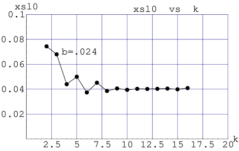
Figure 2.1: A plot of $x_{sl0}$ versus $k$ for the simple one cell lattice with a single multipole of order $k$ at $q_{f}$. $x_{sl0}$ is the largest $x_{0}$ that is stable for 100 periods. $p_{x0}=p_{y0}=y_{0}=0$ and 2 dimensional motion. In the figure xs10 represents $x_{sl0}$ .

One sees that at lower values of $k$, $x_{sl0}$ varies rapidly and then levels out at a value close to $x_{sl0}=R=0.04$. The high multipole limit gives a good approximation for $x_{sl0}$ starting with the relatively low values of $k>10$ for non-linear multipoles of the order of those expected in RHIC. It will be seen below that this property helps to make the high multipole limit useful for estimating the dynamic aperture of an accelerator.

The stability surface at $q_{f}$ for the simple lattice with a single $b_{k}$ at $q_{f}$

The stability boundary in the high multipole limit will now be found for the simple one cell lattice with just one $b_{k}$ at $q_{f}$. To find the stability surface in $x_{0}$, $p_{x0}$, one can search along different directions in $x_{0},p_{x0}$ space to find the stability boundary in that direction. One may write the initial coordinates as

$$x_{0} = (\beta_{x}\ \epsilon_{x0})^{0.5}cos(\alpha\pi/2)$$

$$p_{x0} = (\epsilon_{x0}/\beta_{x})^{0.5}sin(\alpha\pi/2)$$ (2.5)

$\alpha$ gives the direction of search in $x_{0}$, $p_{x0}$ and $\epsilon_{x0}$ is the initial linear emittance for this choice of $x_{0}$. $p_{x0}$ at $q_{f}$ where $\alpha_{x}=0$, $\beta_{x}=68.4497$ m. To do the search $\epsilon_{x0}$ will be increased until the motion becomes unstable for a particular choice of $\alpha$. The value of $\epsilon_{x0}$ that lies on the stability boundary for this search direction will be denoted by $\epsilon_{xsl0}$. According to the basic rule for the high multipole limit, Eq. 2.3, we should find that $\epsilon_{xsl0}$ is constant for all directions at the value $\epsilon_{xsl0}=R^{2}/\beta_{x}=23.37482740$. This would establish the basic rule for this lattice. This tracking study is done with a single field multipole, $b_{k}$, at the middle of $q_{f}$. In order to find the stability boundary for the high multipole limit, $k$ is chosen at the large value of $k=1\cdot 10^{6}$. The results of this tracking study are shown in Table 2.1, where $\epsilon_{xsl0}$ is shown as a function of $\alpha$.

$\alpha$	$\epsilon_{xsl0}$
$-1$	23.3893
$-0.75$	23.3749
$-0.5$	23.3756
$-0.25$	23.3748
$0.$	23.3747
$0.25$	23.386
$0.5$	23.4199
$0.75$	23.4024
$1.$	23.3893

Table 2.1: The linear emittance, $\epsilon_{xsl0}$, computed for different points, $x_{0}$, $p_{x0}$ on the stability boundary in the hml, corresponding to different directions in $x_{0}$, $p_{x0}$ space, at the location of $q_{f}$ in the simple one cell lattice. The parameter $\alpha$ gives the different directions according to Eqs. 2.5. $\epsilon_{xsl0}$ is in mm mrad.

One sees in Table 2.1 that $\epsilon_{xsl0}$ for different directions is almost constant at the value 23.37482740 as predicted by the basic rule. However, there is a variation in $\epsilon_{xsl0}$ of about .2%, which appears to show that the basic rule for high multipole limit, Eq. 2.3, is not exact but has a small error in it. This error is not important for the main results of this paper. This particular study shows that it is convenient to have a precise definition of stability such as is given in section 6.

$x_{slo}$ at $q_{d}$ for the simple lattice with a single $b_{k}$ at $q_{f}$

Our next step will be to consider the stability limit at some other location in the lattice, where $\beta_{x}$ is not at its maximum value, such as at $q_{d}$ where $\beta_{x}$ is $\beta_{x}=21.12345678$. According to the basic rule for the high multipole limit for the simple one cell lattice, the stability limit in $x_{0}$ when $p_{x0}=0$ at $q_{f}$, $x_{sl0f}$, is related to the stability limit at $q_{d}$, $x_{sld}$, at large enough $k$, by

$$x_{sl0d}=(\beta_{xd}/\beta_{xf})^{0.5}\ x_{sl0f}$$ (2.6)

where $\beta_{xf}$ and $\beta_{xd}$ are the beta functions at $q_{f}$ and $q_{d}$. This is illustrated in Table 2.2 where $x_{slf}$ and $x_{sld}$ are compared as a function of $k$, the order of the field multipole at $q_{f}$.

$k$	$x_{slqd}$	$x_{slqf}$	$[x_{slqd}/x_{slqf}]\sqrt{\beta_{xf}/\beta_{xd}}$
1000000	0.02248406	0.03999994	1.0000187
10000000	0.0224841	0.03999999	1.0000193
100000000	0.02248411	0.03999999	1.0000198

Table 2.2: A table showing how well $x_{sl0}$ in the hml varies like $\beta_{x}^{0.5}$ through the lattice. $x_{slo}$ is the largest $x_{0}$ that is stable for 100 periods for the simple one cell lattice when $p_{x0}=0$ with a single multipole of order $k$ at $q_{f}$. $x_{sl0}$ at $q_{f}$ and $q_{d}$ are indicated by $x_{sl0f}$ and $x_{sl0d}$, and $\beta_{xqf}$ and $\beta_{xqd}$ are the linear beta functions at $q_{f}$ and $q_{d}$. All lengths are in meters.

One sees from Table 2.2 that the prediction of the basic rule for this case, as given by Eq. 2.6, is valid with an error of about $2\ 10^{-5}$. The reason for varying $k$ was to show that the error found was not due to $k$ not being large enough as the basic rule for the high multipole limit holds only for large enough $k$ values. The error in computing the beta functions also appears to be too small to account for the error found in Table 2.2.

$x_{slo}$ at $q_{d}$ and $q_{f}$ for the simple lattice with a single $b_{k}$ at $q_{f}$ and a $b_{k}$ at
$q_{d}$ with a different $R$ value

We will now consider the case of the simple one cell lattice with two field multipoles present; one at $q_{f}$ and one at $q_{d}$. The field multipole at $q_{d}$ will have an $R$-value (see Eq. 2.4), $R_{qd}$ which is different from the $R$-value, $R_{qf}$, of the multipole at $q_{f}$. According to the basic rule for the hml, Eq. 2.3, when $R_{qd}=R_{qf}$, the multipole at $qf$ will dominate in determining the hml since $[R^{2}/\beta_{x}]_{\rm min}$ will occur at $q_{f}$ where $\beta_{x}$ has its maximum. In particular, Eq. 2.3 gives $x_{sl0}$ when $p_{s0}=0$ as $x_{sl0f}=R_{qf}$, while $x_{sl0}$ at $q_{d}$ is given by Eq. 2.6 as $x_{sl0d}=\sqrt{[\beta_{xd}/\beta_{xf}]}Rqf$. If one now reduces $R_{qd}$, the multipole at $q_{f}$ will continue to dominate until $R_{qd}$ reaches the value $\sqrt{[\beta_{xd}/\beta_{xf}]}R_{qf}$, and then the multipole at $q_{d}$ will start to dominate, and $x_{sl0d}$ will be given by $R_{qd}$ while $x_{sl0f}$ will be given by $\sqrt{[\beta_{xf}/\beta_{xd}]}R_{qd}$. These results are illustrated by the computed results given in Table 2.3 where $x_{sl0f}$ and $x_{sl0d}$ are shown as $R_{qd}/R_{qf}$ is decreased from 1 to 0.2. For this lattice $R_{qf}$ is held constant at 0.04 m and $\sqrt{[\beta_{xd}/\beta_{xf}]}=0.56209177$.

$R_{qd}/R_{qf}$	$x_{sl0qf}$	$R_{qd}$	$x_{sl0qd}$
1.	0.03999	0.04	0.02248
0.9	0.03999	0.036	0.02248
0.8	0.03999	0.032	0.02248
0.7	0.03999	0.028	0.02248
0.6	0.03999	0.024	0.02248
0.55	0.03914	0.022	0.02199
0.5	0.03558	0.02	0.01999
0.4	0.02846	0.016	0.01599
0.3	0.02134	0.012	0.01199

Table 2.3: A table showing that the stability boundary in the hml is determined by the element in the lattice with the smallest value of $R/\beta_{x}^{0.5}$. Results shown are for the simple one cell lattice with a single multipole with the same order at $q_{f}$ and $q_{d}$. $R_{qf}$, $R_{qd}$ and $x_{sl0f}$, $x_{sl0d}$ are the $R$ and $x_{sl0}$ parameters at $q_{f}$ and $q_{d}$. All lengths are in meters.

It will be suggested below that the high multipole limit provides a reasonable measure of the dynamic aperture. Assuming this to be so, then the basic rule for the hml states that in an accelerator the dynamic aperture is dominated by the magnet with the smallest $R/\beta_{x}^{0.5}$. For example, if an accelerator has 6 insertions with 6 crossing points, with similar magnets that are excited to give different $\beta_{x}$ at the crossing points, the magnet which has the largest $\beta_{x}$ will dominate and determine the dynamic aperture[2]. This magnet is located in the insertion with the smallest $\beta_{x}$ at the crossing point. The dynamic aperture at other locations in the lattice will scale like $(\beta_{x}/\beta_{x{\rm max}})^{0.5}$ where $\beta_{x{\rm max}}$ is the largest $\beta_{x}$ in the lattice.

The dependence of $x_{sl0}$ vs $k$ at $q_{f}$ on the strength of field multipole, $\mathrm{b}$

In the previous tracking studies, the multipole present is assumed to have the form, $b_{k}=\mathrm{b}/R^{k}$, where $\mathrm{b}$ is the integrated strength of the point multipole. $\mathrm{b}$ and $R$ can vary from one element in the lattice to another. The basic rule for the high multipole limit, Eq. 2.3, does not show any dependence on $\mathrm{b}$. Tracking studies show that when $\mathrm{b}$ is increased, the high multipole limit is unchanged, but one must go to a larger value of $k$ before the high multipole limit is reached. The studies also show that for large enough values of $k$, $x_{sl0}$, the largest stable $x_{0}$ when $p_{x0}=0$, goes like $\mathrm{b}^{(1/k)}$. This indicates that for large enough $k$, $x_{sl0}$ is insensitive to the size of $\mathrm{b}$. For RHIC, the high multipole limit is reached for relatively low values of $k$, $k\sim 10$, and this result is insensitive to the size of the non-linear multipoles. Assuming the high multipole limit is a good measure of the dynamic aperture of an accelerator, then the dynamic aperture of an accelerator should be insensitive to the size of the higher multipoles, $k$ larger than 10 for RHIC.

Fig. 2.2 shows $x_{sl0}$ plotted against $k$ for the simple one cell lattice with a single $b_{k}$ at $q_{f}$. The two plots shown are for $\mathbf{b}=0.024$ m and for $\mathbf{b}=0.24$ m.

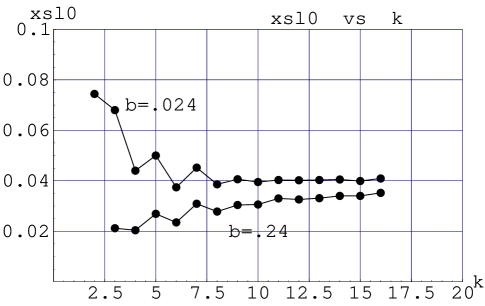
Figure 2.2: A plot showing how $x_{sl0}$ versus $k$ depends on the strength, $\mathbf{b}$, of the single multipole at $q_{f}$ for the simple one cell lattice, by comparing two cases where $\mathbf{b}$ differs by a factor of 10. In the figure xsl0 represents $x_{sl0}$.

One sees that the same high multipole limit is reached at about $k=10$ for $\mathrm{b}=.024$ and about $k=24$ for $\mathrm{b}=0.24$.

Fig. 2.3 shows that $x_{sl0}\sim\mathrm{b}^{(1/k)}$ by plotting $x_{sl0}(0.024)/x_{sl0}(0.24)/10^{(1/k)}$ against $k$. This ratio should approach 1 for large $k$ if $x_{sl0}\sim\mathrm{b}^{(1/k)}$.

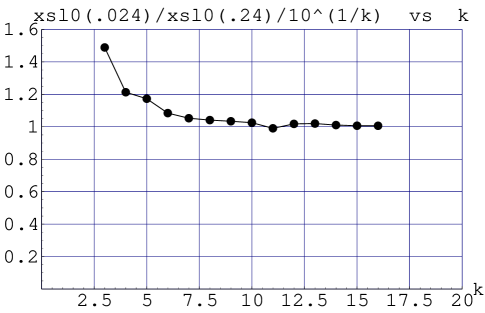
Figure 2.3: A plot showing that $x_{sl0}$ depends on the multipole strength like $x_{sl0}\sim\mathrm{b}^{(1/k)}$ for large $k$, by comparing two cases where $\mathbf{b}$ differs by a factor of 10. In the figure, xsl0 represents $x_{sl0}$.

In the above it was shown that $x_{sl0}\sim\mathbf{b}^{(1/k)}$ which shows the dependence of $x_{sl0}$ on $\mathrm{b}$ for a fixed $k$. A more complete result which also shows the dependence on $k$ is

$$x_{sl0}\sim\mathrm{b}^{(1/k)}/k$$ (2.7)

The dependence of the high multipole limit stability boundary on the choice
of linear tunes, $\nu_{x}$ and $\nu_{y}$

Tracking studies done with the simple one cell lattice indicate that the stability boundary in the high multipole limit does not depend on the choice of linear tunes, $\nu_{x}$ and $\nu_{y}$. This leads to the suggestion, see section 8, that the linear tunes be chosen to avoid the resonances driven by the lower multipoles. The term lower multipoles is defined below.

Chapter 3 The high multipole limit in 4 dimensions

In 2 dimensional phase space motion, the stability boundary that encloses the stable area in $x_{0}$, $p_{x0}$ in the high multipole limit is given by

$$\epsilon(x_{0},p_{x0})=[R^{2}/\beta_{x}]_{\rm min}$$ (3.1)

One may ask what is the stability boundary for motion in 4 dimensional phase space in the high multipole limit. To answer this, one has to consider the motion of a particle moving in a lattice whose only nonlinear field in each element is that of a single multipole given by

$$B_{y}+iB_{x}=-B_{0}\ \mathbf{b}((x+iy)/R)^{k}$$ (3.2)

where $R$ may depend on $s$, and so may $\mathbf{b}$ although not by very large factors. To find the high multipole limit stability boundary, one may use the argument given in section 2. For very large $k$, and for $x^{2}+y^{2}$ not close to $R^{2}$, Eq. 3.2 shows that $B_{y}\sim B_{x}\sim 0$. Thus for $x^{2}+y^{2}$ not close to $R^{2}$,

$$\epsilon_{x}(x,p_{x})=\epsilon_{x0},\qquad\epsilon_{y}(y,p_{y})=\epsilon_{y0}$$ (3.3)

where $\epsilon_{x0}$, $\epsilon_{y0}$ are two constants and $\epsilon_{x}$ and $\epsilon_{y}$ are the linear emittance invariants. In addition for stable motion one has

$$(x^{2}+y^{2})<R^{2}$$ (3.4)

Equation 3.4 can be restated as, using Eq. 3.3,

$$(\beta_{x}\ \epsilon_{x0}+\beta_{y}\ \epsilon_{y0})<R^{2}$$ (3.5)

Eq. 3.4 limits the range of $\epsilon_{x0}$, $\epsilon_{y0}$ for which the motion is stable. On the stability boundary , $\epsilon_{x}$ and $\epsilon_{y}$ are constant with the values of $\epsilon_{x0}$ and $\epsilon_{y0}$ respectively, and for each set of values of $\epsilon_{x0}$ and $\epsilon_{y0}$ that are on the stability boundary, $x^{2}+y^{2}$ must be less than or equal to $R^{2}$ for each element and at some point around the lattice $x^{2}+y^{2}$ must be equal to $R^{2}.$

Eqs. 3.3 through 3.5 define the stability boundary in the high multipole limit. The stability boundary for the high multipole limit may be visualized as a curve in $\epsilon_{x0}$, $\epsilon_{y0}$ space as shown in Fig. 3.1. For motion in 4 dimensional phase space, there does not appear to be a simple solution for the stability boundary in $\epsilon_{x0}$, $\epsilon_{y0}$ space. This solution may depend on the particular form of $\beta_{x}(s)$, $\beta_{y}(s)$. There are, however, 3 points on the stability boundary for which one can find simple results. These are the 3 points for which 1. $\epsilon_{x0}=0$, 2. $\epsilon_{y0}=0$ and 3. $\epsilon_{x0}=\epsilon_{y0}$.

Figure 3.1: A plot showing the stability boundary in the hml for 4 dimensional motion, for the simple one cell lattice, as a plot of $\epsilon_{y0}$ versus $\epsilon_{x0}$. epy0, epx0 represent $\epsilon_{y0}$, $\epsilon_{x0}$.

For the $\epsilon_{y0}=0$ point, Eqs. 3.3 through 3.5 give

$$\epsilon_{x0}=[R^{2}/\beta_{x}]_{\rm min},\qquad\epsilon_{y0}=0$$ (3.6)

as the value of $\epsilon_{x0}$ on the stability boundary when $\epsilon_{y0}=0$. $[R^{2}/\beta_{x}]_{\rm min}$ is the minimum value of $R^{2}/\beta_{x}$ around the lattice. With this value of $\epsilon_{x0}$ and $\epsilon_{y}=0$, one can show that $(x^{2}+y^{2})$ is less than or equal to $R^{2}$ at every element in the lattice. Similarly for $\epsilon_{x0}=0$, one finds

$$\epsilon_{y0}=[R^{2}/\beta_{y}]_{\rm min},\qquad\epsilon_{x0}=0$$ (3.7)

When $\epsilon_{x0}=\epsilon_{y0}$, one finds

$$\epsilon_{x0}=\epsilon_{y0}=[R^{2}/(\beta_{x}+\beta_{y})]_{\rm min}$$ (3.8)

The three points on the stability boundary given by Eqs. 3.6 through 3.8 provide a fairly good picture of the stability boundary. A fairly good approximation can be obtained by drawing two straight lines between the known three points.

For accelerators which have insertion regions where $\beta_{x}$, $\beta_{y}$ have exceptionally large values which occur in magnets which have the same $R$ value, $R_{\rm ins}$, then Eqs. 3.6 through 3.8 can written as

$$\epsilon_{x0} = R_{\rm ins}^{2}/\beta_{x{\rm max}},\qquad\epsilon_{y0}=0$$

$$\epsilon_{y0} = R_{\rm ins}^{2}/\beta_{y{\rm max}},\qquad\epsilon_{x0}=0$$ (3.9)

$$\epsilon_{x0} = \epsilon_{y0}=R_{\rm ins}^{2}/(\beta_{x}+\beta_{y})_{\rm max}$$

$\beta_{x{\rm max}}$ is the largest $\beta_{x}$ in the lattice, and $\beta_{y{\rm max}}$ and $(\beta_{x}+\beta_{y})_{\rm max}$ have similar meanings.

Often, in tracking studies one does runs with initial values $\epsilon_{x0}=\epsilon_{y0}$ and $p_{x0}=0$, $p_{y0}=0$, increasing $x_{0}$ until the motion becomes unstable for a given number of periods. The corresponding value of $x_{0}$ may be labeled $x_{sl0}$. If one does tracking studies where all the $b_{k}$ present have the same $k$ value, then for large enough $k$, the basic rule high multipole limit in 4 dimensions states that $x_{sl0}$ will approach a non-zero value given by Eq. 3.8 as

$$x_{sl0}=\sqrt{(\beta_{x0}/R_{0}^{2})[R^{2}/(\beta_{x}+\beta_{y})]_{\rm min}}$$ (3.10)

where $\beta_{x0}$ and $R_{0}$ are these parameters at the element where $x_{sl0}$ is measured. For the insertion case described by Eq. 3.9, $x_{sl0}$ is given by

$$x_{sl0}=(R_{0}/R_{\rm ins})\sqrt{\beta_{x0}/(\beta_{x}+\beta_{y})_{\rm max}}$$ (3.11)

In Fig. 3.1, $\epsilon_{y0}$ is plotted against $\epsilon_{x0}$ showing the stability boundary in the initial emmitance space of $\epsilon_{x0}$, $\epsilon_{y0}$. This curve was found by a tracking study using the simple one cell lattice with a single $b_{k}$ at $q_{f}$. $k$ was chosen at the large value of $k=1\ 10^{6}$, so that the curve is a good approximation of the high multipole limit. In this case the stability boundary in $\epsilon_{x0}$, $\epsilon_{y0}$ is almost a straight line. A simple approximation of the stability boundary is a straight line connecting the end points, the $\epsilon_{x0}=0$ point and the $\epsilon_{y0}=0$ point. According to Eqs. 3.6 through 3.8 this straight line is given by

$$\epsilon_{x0}/[R^{2}/\beta_{x}]_{\rm min}+\epsilon_{y0}/[R^{2}/\beta_{y}]_{\rm min}=1$$ (3.12)

For the simple one cell lattice used here, where $b_{k}$ is not zero only at the $qf$ element, then $[R^{2}/\beta_{x}]_{\rm min}=R^{2}/\beta_{xqf}$ and $[R^{2}/\beta y]{\rm min}=R^{2}/\beta_{yqf}$, $R=0.04$ m and $\beta xqf=68.4497$, $\beta yqf=21.6265$. One finds in this case that the three points on the stability boundary as given by Eqs. 3.6 through 3.8 agree with the tracking results with an error less than $5\ 10^{-3}$.

One may note that if $[R^{2}/\beta_{x}]_{\rm min}=[R^{2}/\beta_{y}]_{\rm min}$, which is true for RHIC because $\beta x=\beta y$ at the low beta crossing points and tends to be true for proton colliders, then Eq. 3.12 gives

$$\epsilon_{x0}+\epsilon_{y0}={\rm constant}$$ (3.13)

on the stability boundary. Tracking studies indicate that Eq. 3.13 is roughly true for RHIC. Assuming the high multipole limit provides a reasonable estimate of the dynamic aperture of the actual accelerator, then the above shows that the result that the total emittance, $\epsilon_{x0}+\epsilon_{y0}$, is roughly constant on the stability boundary is accidental in the sense that it depends on the properties of the beta functions at the crossing points. If these beta functions are not equal, then Eq.3.12 will replace Eq. 3.13.

Figure 3.2 illustrates the result given by Eq. 3.10 for $x_{sl0}$ for the case when $\epsilon_{x0}=\epsilon_{y0}$, and $p_{x0}=p_{y0}=0$ in the high multipole limit. In fig. 3.2 $x_{sl0}$ is plotted against the multipole order, $k$. The results were found in a tracking study using the simple one cell lattice with a single $b_{k}$ at $q_{f}$. For this lattice, with the parameters used, $R=0.04$ m, and at $q_{f}$, $\beta_{x},\beta_{y}=68.4497$, 21.6265 m. Eq. 3.10 then gives for $x_{sl0}$ at very large $k$, $x_{sl0}=.0349$ m. Fig. 3.2 shows that $x_{sl0}$ is approaching a value at large $k$ near 0.0349m. At $k=20$, $x_{sl0}=.0348$ m was found.

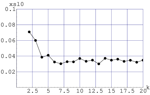
Figure 3.2: A plot of $x_{sl0}$ versus $k$ for the simple one cell lattice with a single multipole of order $k$ at $q_{f}$, for 4 dimensional motion when $p_{x0}=0=p_{y0}$ and $\epsilon_{y0}=\epsilon x0$. In the figure, xsl0 represents $x_{sl0}$ and is in meters.

Chapter 4 High multipole limit and the dynamic aperture

The high multipole limit gives a result for the stability boundary that encloses the stable area in $x_{0}$, $p_{x0}$. The goal of this section is to show that the high multipole limit gives a reasonable approximation for the stability boundary when all the field multipoles are present and the lower multipoles have been corrected. Conversely, the high multipole limit indicates how much may be gained by correcting the lower multipoles. The phrase lower multipoles will be more precisely defined below. Also one will see that when the nonlinear field multipoles are not too large, as is the case in RHIC, the high multipole limit provides a rough but useful estimate of the dynamic aperture.

Motion in 2 dimensional phase space

The above statements can be illustrated by the results of a tracking study in 2 dimensional phase space using the simple one cell lattice with non linear multipoles only at $q_{f}$. To simulate the multipoles present in an accelerator, the point like nonlinear field at $q_{f}$ is given by

$$B_{y}=B_{0}\ mathrm{b}(x/R)^{2}(1-(x/R)^{50})/(1-x/R)$$ (4.1)

Eq. 4.1 gives a nonlinear field which contains all multipoles from $k=2$ to about $k=50$, where all the multipoles decrease like $1/R^{k}$. With the parameters chosen as $R=0.04$m, $\mathrm{b}=0.024$, this lattice resembles the RHIC accelerator without insertions.

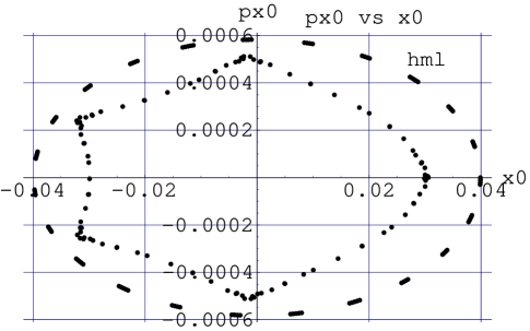
Figure 4.1: A plot of $p_{x0}$ versus $x_{o}$ showing the stability boundary for 2 dimensional motion in the simple one cell lattice with all multipoles from $k=2$ to $k=50$ at $q_{f}$. The stability boundary in the high multipole limit is also shown. In the figure, px0,x0 represent $p_{x0}$, $p_{0}$.

Fig. 4.1 shows the stability boundary in $x_{0}$, $p_{x0}$ space as measured at $q_{f}$. Two boundaries are shown; one is the high multipole limit, and the other boundary, that is contained inside the hml boundary, is the stability boundary when all the multipoles are present as given by Eq. 4.1. According to the suggestions made at the beginning of this section, the difference between these two boundaries shows the loss in stable phase space due to the lower multipoles, and also how much phase space can be gained by correcting the lower multipoles.

The term lower multipoles will be defined as follows. If one looks at Fig. 2.1 and Fig. 3.2 which plot $x_{sl0}$ vs $k$ for the two cases, $\epsilon_{y0}=0$ and $\epsilon_{y0}=\epsilon x0$, one sees that $x_{sl0}$ gets close to the value given by the high multipole limit at about $k=10$ for the simple one cell lattice. This value of $k$ where $x_{sl0}$ gets close to the value given by the hml will be called $k_{\rm hml}$. The lower multipoles are those multipoles for which $k$ is less than $k_{\rm hml}$. Let us now correct the lower multipoles from $k=2$ to $k=9$ giving the plot shown in Fig. 4.2.

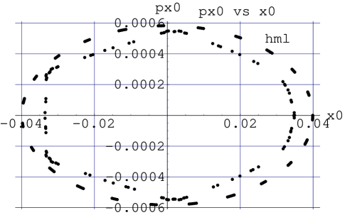
Figure 4.2: A plot of $p_{x0}$ versus $x_{o}$ showing the stability boundary for 2 dimensional motion in the simple one cell lattice with multipoles from $k=10$ to $k=50$ at $q_{f}$. The lower multipoles, $k=2$ to $k=9$ have been corrected. The stability boundary in the high multipole limit is also shown. In the figure, px0,x0 represent $p_{x0}$, $x_{0}$.

Fig. 4.2 shows that by correcting $b_{2}$ to $b_{9}$, the stable phase space area has been increased so that it lies fairly close to the high multipole limit result, but still lies within the high multipole limit. If one corrects more multipoles past $b_{9}$, the stability boundary will increase approaching the result for the high multipole limit. Results found using a RHIC lattice will be presented in section 6 which will also support the validity of the suggestions made in this section about the connection between the dynamic aperture and the high multipole limit. One may note that Fig. 4.1 shows that the loss in stable phase space due to the non linear multipoles used is about a factor of 2. About the same factor will be found for a RHIC lattice. Thus one can say that the hml provides a rough but useful estimate of dynamic aperture when the multipoles present are of the order of those expected in RHIC, overestimating the stable phase area in 2 dimensional phase space by about a factor of 2.

Motion in 4 dimensional phase space

The suggestions made at the beginning of this section can be illustrated by the results of a tracking study in 4 dimensional phase space using the simple one cell lattice with nonlinear multipoles only at $q_{f}$. To simulate the multipoles present in an accelerator, the point like nonlinear field at $q_{f}$ is given by

$$B_{y}+iB_{x}=B_{0}\ \mathrm{b}((x+iy)/R)^{2}(1-(x+iy)/R)^{50})/(1-(x+iy)/R)$$ (4.2)

Eq. 4.2 gives a nonlinear field which contains all multipoles from $k=2$ to about $k=50$, where all the multipoles decrease like $1/R^{k}$. With the parameters chosen as $R=0.04$m, $\mathrm{b}=0.024$, this lattice resembles the RHIC accelerator without insertions.

Fig. 4.3 shows the stability boundary in $\epsilon_{x0}$, $\epsilon_{y0}$ space as measured at $q_{f}$. Two surfaces are shown; one is the high multipole limit, and other surface, that is contained within the high multipole limit surface, is the stability boundary when all the multipoles are present as given by Eq. 4.2. According to the suggestions made at the beginning of this section, the difference between these two boundaries shows the loss in stable phase space due to the lower multipoles, and also how much phase space can be gained by correcting the lower multipoles.

Figure 4.3: A plot of $\epsilon_{y0}$ versus $\epsilon_{x0}$ showing the stability boundary in $\epsilon_{x0}$, $\epsilon_{y0}$ space for 4 dimensional motion in the simple one cell lattice when all the multipoles from $k=2$ to $k=50$ are present at $q_{f}$. The stability boundary in the high multipole limit is also shown. In the figure, epy0,epx0 represent $\epsilon_{y0}$, $\epsilon_{x0}$.

One may note that the high multipole limit stability boundary in $\epsilon_{x0}$, $\epsilon_{y0}$ space is a curve with zero thickness. However for the simple one cell lattice with all the multipoles present the $\epsilon_{y0}$ vs $\epsilon_{x0}$ stability curve has a certain smear or non-zero thickness. This is because for a choice of $\epsilon_{x0}$, the $\epsilon_{y0}$ that lies on the stability boundary depends on the choice of $x_{0}$, $p_{x0}$, $y_{0}$, $p_{y0}$. The curve shown in Fig. 4.3 was obtained with $p_{x0}=p_{y0}=0$.

Let us now correct the lower multipoles from $k=2$ to $k=9$ giving the plot shown in Fig. 4.4. Fig. 4.4 shows that by correcting $b_{2}$ to $b_{9}$, the stable phase space area has been increased so that it lies fairly close to the high multipole limit result, but still lies within the high multipole limit boundary. If one corrects more multipoles past $b_{9}$, the stability boundary will increase approaching the result for the high multipole limit. Results found using a RHIC lattice will be presented in section 5 which will also support the validity of the suggestions made in this section about the connection between the dynamic aperture and the high multipole limit. The results shown in Figs. 4.3, and  4.4 also show how one can obtain misleading conclusions by looking at the results for just one direction in $\epsilon_{x0}$, $\epsilon_{yo}$ space like the $\epsilon_{x0}=\epsilon_{y0}$ direction. In this case the dynamic aperture actually became smaller for this direction when the $k=2$ to 9 multipoles were corrected.

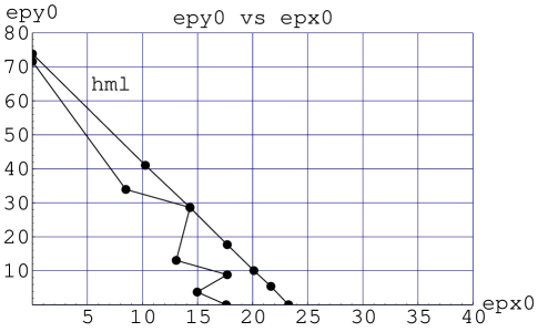
Figure 4.4: A plot of $\epsilon_{y0}$ versus $\epsilon_{x0}$ showing the stability boundary in $\epsilon_{x0}$, $\epsilon_{y0}$ space for 4 dimensional motion in the simple one cell lattice when the multipoles from $k=10$ to $k=50$ are present at $q_{f}$. The multipoles from $k=2$ to $k=9$ have been corrected. The stability boundary in the high multipole limit is also shown. In the figure, epy0,epx0 represent $\epsilon_{y0}$, $\epsilon_{x0}$.

Chapter 5 RHIC lattice results

This section will illustrate the suggestions made in section 4 that the high multipole limit gives a reasonable estimate of the dynamic aperture when the lower multipoles are corrected by giving the results of tracking studies done with an early version of the RHIC lattice [3]. This lattice has random non linear multipoles in each element from $k=2$ up to and including order $k=20$. Skew multipoles are also present. The lattice has 6 insertions with 6 low beta crossing points at which $\beta_{x}=6$ m and $\beta_{x{\rm max}}=236$m, $\beta_{y{\rm max}}=236$m, $(\beta_{x}+\beta_{y})_{\rm max}=309$ m. At $q_{f}$ in the normal cell, where $x$, $p_{x}$, $y$, $p_{y}$ are observed, $\beta_{x}=56$ m, $\beta_{y}=8.72$m.

The high multipole limit in RHIC

In RHIC, the random multipoles in each element decrease roughly as $R^{k}$. Because the multipoles are chosen randomly corresponding to given rms values [3], multipoles of different order or different $k$ values, have different strengths or different $\mathbf{b}$ values. Elements with different $R$ values are also present. The elements that have the smallest values of $R^{2}/\beta_{x}$ or $R^{2}/\beta_{y}$, and which are the dominant elements, are in the insertions at the locations of $\beta_{xmx}$ and $\beta_{ymx}$. The RHIC lattice differs from the simple one cell lattice in the presence of the chromaticity correcting sextupoles. In RHIC, besides the random multipoles whose rms values decrease like $1/R^{k}$, there is also a set of multipoles, the chromaticity correcting sextupoles, which do not fit into the $1/R^{k}$ pattern of the random multipoles. Because of this, it is necessary to change the definition of the high multipole limit for RHIC. As described above, the high multipole limit is found by doing a series of tracking studies in which all the elements of the lattice have one multipole present of the same order, $k$, and the particle motion for very large $k$ is the high multipole limit. In the case of RHIC this procedure is changed in that in each tracking study the chromaticity correcting sextupoles are present as well as the random multipoles of order $k$. With this change in the definition of the high multipole limit, it is again suggested that the high multipole limit gives a reasonable estimate of the dynamic aperture when the lower multipoles are corrected. This will be illustrated by the following tracking results found using a RHIC lattice. This procedure for defining the high multipole limit can be used for any lattice for which there is another nonlinear field present as well as a set of multipoles that decrease like $1/R^{k}$; for example, one systematic multipole may be exceptionally large.

This new definition of the high multipole limit changes the results found in sections 2 and 3 for the stability boundary in the high multipole limit. For very large $k$, and for $x^{2}+y^{2}$ smaller than $R^{2}$ in each element, the particle motion is that of a particle in the presence of the chromaticity correcting sextupoles. In addition for stable motion one has

$$(x^{2}+y^{2})<R^{2}$$ (5.1)

To find the stability boundary, one needs to know what is the maximum value of $x^{2}+y^{2}$ for a given $x_{0}$, $p_{x0}$, $y_{0}$, $p_{y0}$. In section 3, this was given by the linear beta functions. In effect, one has to know what corresponds to the beta functions for the chromaticity correcting sextupoles for computing the maximum value of $x^{2}+y^{2}$. A semi-empirical solution of this problem will given below. One might notice one needs to answer this question only if one wants to have analytical results for points on the stability boundary in the high multipole limit like those given by Eqs. 3.6 through  3.8. One can always find the stability boundary in the high multipole limit with tracking studies without much difficulty.

Fig. 5.1 shows $x_{sl0}$ plotted against $k$. In this study each element contains only one multipole of order $k$, and the multipoles in all the elements all have the same $k$ value and the chromaticity correcting sextupoles are also present. Two curves are shown. For one curve $\epsilon_{y0}=0$, and for the second curve, $\epsilon_{y0}=\epsilon_{x0}$.

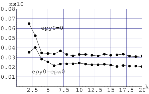
Figure 5.1: A plot of $x_{sl0}$ versus $k$ for RHIC. Each element has a single multipole of the same order, $k$. For one curve $\epsilon_{y0}=0$ and $p_{x0}=p_{y0}=0$. For the other curve $\epsilon_{y0}=\epsilon_{x0}$ and $p_{x0}=p_{y0}=0$. $x_{sl0}$ is computed for 500 turns. In the figure, xsl0,epy0,epx0 represent $x_{sl0}$, $\epsilon_{y0}$, $\epsilon_{x0}$.

$x_{sl0}$ is the largest $x_{0}$ that is stable for 500 turns when $p_{y0}=p_{x0}=0$. Fig. 5.1 is similar to Fig. 3.2 found for the simple one cell lattice and shows that $x_{sl0}$ approaches a non zero limit as $k$ becomes large. Using the results found by tracking runs one can find a result for computing $x_{sl0}$ or $y_{sl0}$ in the high multipole limit in RHIC. For the case when the chromaticity correcting sextupoles are absent, $x_{sl0}$ and $y_{sl0}$ are given by Eq. 3.9 as

$$x_{sl0} = (R_{0}/R_{\rm ins})\sqrt{\beta_{x0}/\beta_{x{\rm max}}},\quad\epsilon_{y0}=0$$

$$x_{sl0} = (R_{0}/R_{\rm ins})\sqrt{\beta_{x0}/(\beta_{x}+\beta_{y})_{\rm max}},\quad\epsilon_{y0}=\epsilon_{x0}$$ (5.2)

$$y_{sl0} = (R_{0}/R_{\rm ins})\sqrt{\beta_{y0}/\beta_{y{\rm max}}},\quad\epsilon_{x0}=0$$

where $\beta_{x0}$, $\beta_{y0}$ and $R_{0}$ are these parameters at the element where $x_{sl0}$ is measured and for the insertion case described in section 3. To obtain a result that may be valid when chromaticity correcting sextupoles are present, we will replace Eqs. 5 by

$$x_{sl0} = f_{1}\ (R_{0}/R_{\rm ins})\sqrt{\beta_{x0}/\beta_{x{\rm max}}},\quad\epsilon_{y0}=0$$

$$x_{sl0} = f_{2}\ (R_{0}/R_{\rm ins})\sqrt{\beta_{x0}/(\beta_{x}+\beta_{y})_{\rm max}},\quad\epsilon_{y0}=\epsilon_{x0}$$ (5.3)

$$y_{sl0} = f_{3}\ (R_{0}/R_{\rm ins})\sqrt{\beta_{y0}/\beta_{y{\rm max}}},\quad\epsilon_{x0}=0$$

In Eq. 5.3, $f_{1}$, $f_{2}$, $f_{3}$ can be found by using the results for $xsl0$ and $ysl0$ found with tracking studies done for RHIC. This gives the results

$$x_{sl0} = (R_{0}/R_{\rm ins})\sqrt{\beta_{x0}/\beta_{x{\rm max}}},\quad\epsilon_{y0}=0$$

$$x_{sl0} = 0.707(R_{0}/R_{\rm ins})\sqrt{\beta_{x0}/(\beta_{x}+\beta_{y})_{\rm max}},\quad\epsilon_{y0}=\epsilon_{x0}$$ (5.4)

$$y_{sl0} = (R_{0}/R_{\rm ins})\sqrt{\beta_{y0}/\beta_{y{\rm max}}},\quad\epsilon_{x0}=0$$

Eqs. 5.4 may be understood in the following way. The chromaticity correcting sextupoles in RHIC do not greatly distort the particle motion. The stability surface in 2 dimensional phase space is a mildly distorted ellipse, as will be seen below. The main effect of the chromaticity correcting sextupoles is due to the coupling of the $x$ and $y$ motions, so that $x^{2}+y^{2}$ will grow from $x_{0}^{2}+y_{0}^{2}$ by a factor which is found to be close to 1.414. Thus in Eqs. 5.4, the $\epsilon_{y0}=0$ and the $\epsilon_{x0}=0$ results are unchanged from those found when the chromaticity correcting sextupoles are absent, while in the $\epsilon_{x0}=\epsilon_{y0}$ case, the $x,y$ coupling changes the result for $xsl0$ by the factor 0.707. Although Eqs. 5.4 were found using tracking results for RHIC, they may be used for other proton storage rings when the chromaticity correcting sextupoles play about the same role in distorting the particle motion. Note that the factor of 0.707 in Eqs. 5.4 is not based on analytical considerations, but was found though tracking studies with RHIC.

Fig. 5.2 shows the stability boundary in the high multipole limit for motion in 2 dimensional phase space, $\epsilon_{y0}=0$. Tracking runs of 500 turns were used. The stability boundary is almost elliptical, showing that the chromaticity correcting sextupoles do not distort the motion very much.

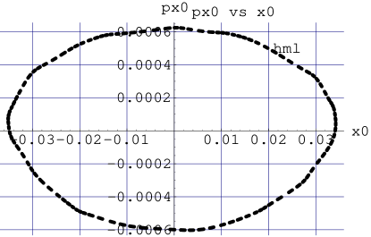
Figure 5.2: A plot showing the stability boundary for 500 turns in the high multipole limit for motion in 2 dimensional phase space for a RHIC lattice. In the figure, px0,xo represent $p_{x0}$, $x_{0}$.

Fig. 5.3 shows the stability boundary in the high multipole limit for motion in 4 dimensional phase space, in $\epsilon_{y0}$ vs $\epsilon_{x0}$ space. Tracking runs of 500 turns were used with $p_{x0}=p_{y0}=0$ and with a single multipole with $k=20$ present in each element. This surface has some thickness or smear which can be found by doing tracking runs with $p_{x0}$ and $p_{y0}$ not 0. This curve is almost a straight line, and using Eqs. 5.3, it is described very well by Eq. 3.12 which in this case can be written as

$$\epsilon_{x0}/[R_{\rm ins}^{2}/\beta_{xmx}]+\epsilon_{y0}/[R_{\rm ins}^{2}/\beta_{ymx}]=1$$ (5.5)

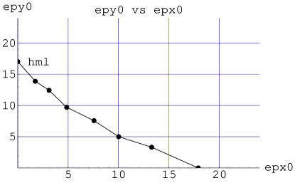
Figure 5.3: A plot showing the stability boundary in the high multipole limit for motion in 4 dimensional phase space for a RHIC lattice in $\epsilon_{y0}$ vs $\epsilon_{x0}$ space. Tracking runs of 500 turns were used with $p_{x0}=p_{y0}=0$ and with a single multipole with $k=20$ present in each element. In the figure, epy0,epx0 represent $\epsilon_{x0}$, $\epsilon_{x0}$ which are in mm mrad.

Motion in 2 dimensional phase space

Tracking studies were done with a RHIC lattice to find the stability boundary for motion in 2 dimensional phase space, $y_{0}=p_{y0}=0$. The results are shown in Fig. 5.4. Two curves are shown. The outer curve is the stability boundary in the high multipole limit as was shown in Fig. 5.2. The inner curve is the path in $x,p_{x}$ for the last $x_{0}$ that was stable for 500 turns as one increased $x_{0}$ with $p_{x0}=0$ and all the multipoles from $k=2$ to $k=20$ are present. According to the suggestion being made here about the significance of the high multipole limit stability boundary, one would say that the lower multipoles have reduced the stable phase space by about 36%. This loss in phase space can be recovered by correcting the lower multipoles, $k$ less than about 10. Again, it is suggested here that the high multipole limit stability boundary indicates the stable phase space when the lower multipoles are corrected and it indicates the loss in phase space due to the lower multipoles.

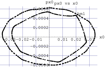
Figure 5.4: A plot showing the stability boundary for 500 turns for 2 dimensional motion in RHIC with all the multipoles from $k=2$ to $k=20$ present. The stability boundary in the high multipole limit is also shown. In the figure, px0,x0 represent $p_{x0}$, $x_{0}$.

Fig. 5.5 is similar to Fig. 5.4 except that the multipoles from $k=2$ to $k=10$ have been omitted. One sees that as the lower multipoles are corrected, the stability boundary approaches that of the high multipole limit. The loss in phase space has now been reduced to about 10%. Particle motions that came even closer to the hml and appeared to be stable for 500 turns were seen and were rejected because of a rather large smear and scatter.

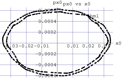
Figure 5.5: A plot showing the stability boundary for 500 turns for 2 dimensional motion in RHIC with the multipoles from $k=11$ to $k=20$ present. The multipoles for $k=2$ to $k=10$ have been corrected. The stability boundary in the high multipole limit is also shown. In the figure, px0,x0 represent $p_{x0}$, $x_{0}$.

Motion in 4 dimensional phase space

Fig. 5.6 shows the results of tracking studies done with a RHIC lattice to find the stability boundary for motion in 4 dimensional phase space. The stability boundary is shown by plotting $\epsilon_{y0}$ versus $\epsilon_{x0}$ for the case where $p_{x0}=p_{y0}=0$. Two curves are shown. The outer boundary is the stability boundary in the high multipole limit. The inner boundary is the stability boundary when all the multipoles from $k=2$ to $k=20$ are present. The hml boundary was found by having only the $k=20$ multipole present. Fig. 5.6 shows a loss in 4 dimensional phase space of about 40% due to the presence of the lower multipoles.

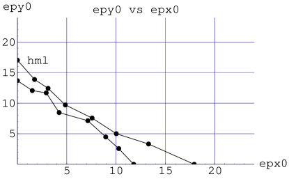
Figure 5.6: A plot showing the stability boundary for 500 turns for 4 dimensional motion for a RHIC lattice with all the multipoles from $k=2$ to $k=20$ present. The stability boundary in the high multipole limit is also shown. In the figure, epy0,epx0 represent $\epsilon_{y0}$, $\epsilon_{x0}$ are in mm-mrad.

Fig. 5.7 shows the result when the multipoles from $k=2$ to $k=10$ are corrected. One sees that as one corrects the lower multipoles, the stability boundary approaches the high multipole limit stability boundary, and the loss in 4 dimensional phase space is reduced to about 10%.

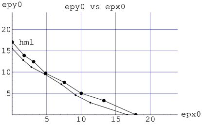
Figure 5.7: A plot showing the stability boundary for 500 turns for 4 dimensional motion for a RHIC lattice with the multipoles from $k=11$ to $k=20$ present. The multipoles for $k=2$ to $k=10$ have been corrected. The stability boundary in the high multipole limit is also shown. In the figure epy0,epx0 represent $\epsilon_{y0}$, $\epsilon_{x0}$ and are in mm-mrad.

Chapter 6 Definition of stability

In order to establish the properties of the high multipole limit, it is convenient to have a definition of stable motion which allows the stability boundary to be determined precisely. In considering the motion of a particle in an accelerator, one might consider the particle motion for a certain number of periods to be stable if the particle motion stays within certain bounds, like those given by the vacuum tank, to be acceptable for the operation of the accelerator. Such a definition of stable motion, which allows a particular amount of acceptable growth in the particle motion, is not convenient for establishing the properties of the high multipole limit. A definition of stable motion is given below which will precisely determine whether a particle motion for a given number of periods is stable. This definition may seem artificial. However, a good deal of numerical tracking shows that the stability limits found using this definition are usually close to the stability limits that would be acceptable for an accelerator.

Consider the motion of a particle in a coordinate system which is based on a reference orbit where the independent coordinate is taken to be $s$, the distance along the reference orbit. The position of the particle is then described by $x$, $y$, and $s$, where $x$, $y$ are the coordinates along two directions perpendicular to the reference orbit. The components of the momentum are then given by $p_{x}$, $p_{y}$ and $p_{s}$. If the energy of the particle is assumed to remain constant during the tracking, then $p_{s}$ can be computed from $p_{s}=(p^{2}-p_{x}^{2}-p_{y}^{2})^{0.5}$, $p$ being the total momentum of the particle. The motion of the particle over a given number of periods will be said to be unstable if during the tracking of the particle over the given number of periods, $p_{s}$ becomes imaginary or $p_{x}^{2}+p_{y}^{2}$ becomes larger than $p^{2}$. $p_{s}$ becoming imaginary means that the formulation of the equations of motion based on the given reference orbit has broken down because $p_{s}$ has changed sign, and the particle has reversed its direction along the reference orbit so that $s$ is decreasing with time.

The above definition of unstable motion over a given number of periods may seem artificial. However it has the advantage that the stability of a particular particle motion over a given number of periods can be precisely determined. Much experience with tracking also indicates that it is a useful definition and usually gives results that are close to the stability limits that would be acceptable for an accelerator. This definition of stability is convenient for establishing the above results for the high multipole limit. This precise definition of stability allows the stability limit to be calculated with great accuracy, and the tracking searches for the stability boundary can be automated. In order to use this definition of stability, one has to use the exact equations of motion. If one uses the approximations often used for large accelerators, where the radical $(p^{2}-p_{x}^{2}-p_{y}^{2})^{0.5}$ is expanded out assuming that $p_{x}/p$ and $p_{y}/p$ are much smaller than one, one will obtain invalid results as the expansion is not valid when $p^{2}-p_{x}^{2}-p_{y}^{2}$ is near zero and the radical is about to become imaginary.

The definition of stability being proposed here has the following advantages:

1. It avoids having to decide whether a particular particle motion is unstable when some growth occurs and it is not obvious whether the growth is acceptable or not.

2. With this definition of stability tracking searches for points on the stability boundary can be automated as it provides a simple test for stability.

The results found in this paper do not depend on the choice of this definition of stability. The same results woud be found with any other reasonable definition of stability.

Chapter 7 Transfer functions for lattice elements

In doing the tracking studies, one needs to know the transfer functions for each element of the lattice. The transfer functions allow one to compute the final coordinates of the particle from the initial coordinates for each element. As was indicated in section 6, the transfer functions have to satisfy the exact equations of motion in order to use the definition of stability given in section 6. This can be accomplished by using the procedure [4] of replacing a magnet with point magnets at the ends of the magnet separated by a drift space. By breaking the magnet up into pieces, one can approach the exact solution of the equations of motion by making the pieces smaller. One change in this procedure will be used here, which is that the reference orbit used will be made up of a series of smoothly joining straight lines and circular arcs [5]. The transfer functions are then given in Ref. [5]. The circular arcs of the reference orbit are located at the dipoles in the lattice, and each arc has the curvature $\rho$ which depends on the strength of the dipole. $1/\rho=0$ at the quadrupoles and drift spaces.

It is assumed that each magnet is broken up into a number of pieces. A magnet piece going from $s=s_{1}$ to $s=s_{2}$ and of length $h=s_{2}-s_{1}$ is replaced by point magnets at the ends separated by a drift space of length $h$. In the following, $q_{x}=p_{x}/p$, $q_{y}=p_{y}/p$, $q_{s}=(1-q_{x}^{2}-q_{y}^{2})^{0.5}$.

A.  Transfer functions for point magnets

The transfer functions for a point magnet located at $s=s_{1}$ is

$$x_{2} = x_{1},\ \ y_{2}=y_{1},$$

$$q_{x2} = q_{x1}+{1\over B\rho}{h\over 2}(1+x_{1}/\rho){\sin\theta\over\theta}B_{y}(x_{1},y_{1}),$$ (7.1)

$$q_{y2} = q_{y1}-{1\over B\rho}{h\over 2}(1+x_{1}/\rho){\sin\theta\over\theta}B_{x}(x_{1},y_{1}),$$

$h$ is the length of the magnet piece, $\theta=h/\rho$. The field components $B_{y}$ and $B_{x}$ are assumed to depend only on $x$, $y$ and do not change along the magnet, and that $B_{s}=0$.

B.  Transfer functions for drift spaces

For a region along $s$ in the lattice where $1/\rho=0$ for the reference orbit

$$q_{x2} = q_{x1},\ \ x_{2}=x_{1}+q_{x1}L_{12},$$

$$q_{y2} = q_{y1},\ \ y_{2}=y_{1}+q_{y1}L_{12},$$

$$L_{12} = (s_{2}-s_{1})/q_{s1}$$ (7.2)

$$q_{s} = (1-q_{x}^{2}-q_{y}^{2})/^{1/2},$$

$L_{12}$ is the path length between $s_{1}$ and $s_{2}$.

For a region where $1/\rho$ is not zero,

$$q_{x2} = q_{x1}\cos\theta+q_{s1}\sin\theta,$$

$$q_{s2} = -q_{x1}\sin\theta+q_{s1}\cos\theta,$$

$$\theta = (s_{2}-s_{1})/\rho,$$

$$x_{2} = x_{1}+(1+x_{1}/\rho)2\rho\sin(\theta/2)$$

$$\qquad\mbox{}\times{q_{x1}\cos\theta/2+q_{s1}\sin\theta/2\over-q_{x1}\sin\theta+q_{s1}\cos\theta},$$

$$L_{12} = (1+x_{1}/\rho)\rho\sin(\theta)/q_{s2},$$

$$q_{y2} = q_{y1},\ \ y_{2}=y_{1}+q_{y1}L_{12}$$

C.  Transfer functions for the simple one cell lattice

This lattice has only point quadrupoles and drift spaces. For the transfer functions of the point quadrupoles one can use Eqs. 7.1, replacing $(h/2)B_{y}$ and $(h/2)B_{x}$ by the integrated fields of the point magnet. For the drift spaces one can use Eqs. 7.2. The initial parameters that were used for the simple one cell lattice are the following:

quadrupole integrated strength = 436.647 KG

drift space length = 20m

multipole field, $b_{k}=\mathrm{b}\ /\ R^{k}$, $\mathrm{b}=0.024$,  $R=0.04$m

$B\rho=8400$ KG. m

$B_{0}=35$ KG

Chapter 8 Longterm effects and the high multipole limit

The stability boundary in the high multipole limit for 2 dimensional phase space does not appear to depend on nprd, the number of periods the particle is tracked. However many tracking studies have indicated that the stability boundary shrinks slowly the longer the particle is tracked. If one accepts the statement that the stability boundary in the high multipole limit is the boundary that is approached when the lower multipoles are corrected, then one can remove the apparent contradiction by the suggestion that the shrinking of the stability boundary, when nprd is increased, is due to the presence of the lower multipoles, and this effect can be reduced by correcting the lower multipoles.

The following tracking study done with the simple one cell lattice supports the previous statements. If one considers $x_{sl0}$, the largest $x0$ that is stable for a given number of periods when $p_{x0}=0$, then one finds that $x_{sl0}$ decreases as nprd is increased. Using nprd $=10^{2}$ and nprd $=10^{4}$, one finds the $dx_{0}/x_{0}$, the fractional decrease in $x_{sl0}$ for these two values of nprd is $dx_{0}/x_{0}=0.033$ when all the multipoles are present. If one corrects some of the lower multipoles by omitting the multipoles for k=2 to k=9, then one finds that $dx_{0}/x_{0}$ is decreased by a factor of 6 to $dx_{0}/x_{0}=0.005$.

Avoiding resonances of order 10 or higher

It is sometimes suggested that in choosing the operating point for superconducting proton storage rings, one should avoid resonances of order 10 or higher. A basis for this rule is provided by the high multipole limit. The range of the lower multipoles that reduce the dynamic aperture below that given by the high multipole limit is given by the parameter $k_{hml}$ defined in section 4. For RHIC, $k_{hml}$ is about $k_{hml}=10$. Since the important multipoles in affecting the dynamic aperture are the 10 lowest multipoles, it would seem desirable to avoid resonances up to 10 or higher which are the resonances driven by the 10 lowest multipoles in lowest order. If one would increase the strength of the non-linear multipoles by a factor of 10, thus raising $k_{hml}$ to about $k_{hml}=20$, the above argument would suggest that one should avoid resonances up to order 20 or higher.

Bibliography

- [1] G. Parzen, Higher order magnet field multipoles, aperture effects and tracking studies, BNL report RHIC-AP-25 (1986).
- [2] G. Parzen, Dynamic aperture for lattices with some beta = 2 insertions, BNL report AD/RHIC-AP-75 (1989).
- [3] Conceptual design of RHIC, BNL report BNL-52195, (1989).
- [4] L. Schachinger and R. Talman. Teapot, A thin element tracking program, SSC-52 (1985).
- [5] G. Parzen, Symplectic tracking using point magnets and a reference orbit of circular and straight lines. Phys. Rev. E ,Vol. 51, No.3, p. 51 (1995).