UV continuum emission and diagnostics
of hydrogen-containing non-equilibrium plasmas

Abstract

For the first time the emission of the radiative dissociation continuum of the hydrogen molecule ($a^{3}\Sigma_{g}^{+}\to b^{3}\Sigma_{u}^{+}$ electronic transition) is proposed to be used as a source of information for the spectroscopic diagnostics of non-equilibrium plasmas. The detailed analysis of excitation-deactivation kinetics, rate constants of various collisional and radiative transitions and fitting procedures made it possible to develop two new methods of diagnostics of: (1) the ground $X^{1}\Sigma_{g}^{+}$ state vibrational temperature $T_{\text{vib}}$ from the relative intensity distribution, and (2) the rate of electron impact dissociation $(d[\mbox{H${}_{2}$}]/dt)_{\text{diss}}$ from the absolute intensity of the continuum. The known method of determination of $T_{\text{vib}}$ from relative intensities of Fulcher-$\alpha$ bands was seriously corrected and simplified due to the revision of $d\to a$ transition probabilities and cross sections of $d\leftarrow X$ electron impact excitation. General considerations are illustrated with examples of experiments in pure hydrogen capillary-arc and H₂+Ar microwave discharges. In pure H₂ plasma the values of $T_{\text{vib}}$ obtained by two independent methods are in rather good accordance ($T_{\text{vib}}$=3000-5000 K). In the H₂+Ar microwave plasma it was observed for the first time that the shape of the continuum depends on the ratio of the mixture components. Absorption measurements of the population of the 3s²3p⁵4s levels of Ar together with certain computer simulations showed that the Ar*$\to$H₂ excitation transfer plays a significant role. In our typical conditions (power flux: 4 W cm^-2, pressure $p=0.5$ mbar, H₂:Ar=1:1) the following values were obtained for the microwave discharge: $(d[\mbox{H${}_{2}$}]/dt)_{\text{diss}}\approx 2.5-5\cdot 10^{17}$ cm^-3 s^-1. The contribution of the excitation transfer is about 10-30% of the total population of the $a^{3}\Sigma_{g}^{+}$ state.

I Introduction

Experimental and theoretical studies of the emission of the H₂ radiative dissociation continuum ($a^{3}\Sigma_{g}^{+}\to b^{3}\Sigma_{u}^{+}$ electronic transition) have a long and interesting history. They were stimulated by molecular spectroscopy and quantum chemistry [1, 2, 3, 4, 5, 6, 7], investigations of hydrogen containing plasmas [8, 9, 10] and astrophysics [11, 12]. Since the first work of Houtermans [13] the $a^{3}\Sigma_{g}^{+}\to b^{3}\Sigma_{u}^{+}$ transition has been studied as a possible laser system (see [14, 15, 16, 17] and Refs. therein). It is widely used in UV and VUV light sources [8, 18, 19, 20, 21].

In spite of numerous studies, the H₂ continuum emission was never used or even proposed to be used for a determination of plasma parameters, i.e., for spectroscopic plasma diagnostics. It seems to be rather strange because, on one hand, diagnostics of hydrogen-containing plasmas is not trivial and every opportunity should be tried; on the other hand, emission spectroscopy due to its passive nature and instrumental simplicity is of primary interest for various studies in plasma physics and industrial applications. Moreover the visible spectrum of hydrogen plasma gives us in principle only three qualitatively different sources of information: (1) atomic lines of Balmer series, (2) band (actually multi-line) spectrum of H₂, and (3) the continuum. First two are successfully used in plasma diagnostics, while the third one was never even tried. Previous investigators only measured the continuum intensity and sometimes made certain calculations for comparison with an experiment [9, 10]. It should be underlined that those calculations are solutions of so-called direct problem of spectroscopy (from known plasma parameters to observable spectrum).

It is obvious that any observable property of plasma is somehow connected with values of plasma parameters and therefore in principle may be tried to be used as a diagnostic tool. However actually, as a rule, one observable quantity is determined by several different plasma parameters. Then the key point is to study the informational content of experimental data and to find the proper way of data analysis. The last one is always an inversion problem (from an observed spectrum to unknown plasma parameters) having its own specifics (see below section II).

The main goal of the present work was to investigate the possibility to use H₂ continuum intensity for diagnostics of non-equilibrium plasmas. Our decision to make the first steps in this direction was based on following a priory considerations. The experimental data on the continuum intensity may be considered as two different sources of information: the relative spectral distribution and the total absolute intensity of the continuum.

The first one is directly connected with the population density distribution over vibrational levels of the $a^{3}\Sigma_{g}^{+}$ state. In low pressure plasmas the levels are populated predominantly by direct electron impact excitation and the deactivation is mainly due to spontaneous emission [9, 10]. In this case the relation between the vibrational population density distributions in excited and ground electronic states should be obtained within corona-like models. So the shape of the continuum should be usable for a determination of the vibrational density distribution (or at least the vibrational temperature) of the ground state of H₂.

On the other hand every act of the continuum emission leads to a dissociation of a hydrogen molecule. Therefore, an absolute value of the continuum intensity is directly connected with the rate of radiative dissociation via the $a^{3}\Sigma_{g}^{+}$ state and also may be used for an estimation of the total rate of electron impact dissociation.

Our intention was to investigate both opportunities and to check them experimentally. Therefore the present work includes two closely connected tasks (development of new methods and their test in certain real plasma conditions) and two groups of results connected with the proposed methods and with non-equilibrium plasma of the discharges under the study.

The first part is based on the analysis and description of:

1. excitation-deactivation kinetics and derivation of suitable formulas (Sections II.1, II.2, II.4, IV.3);

2. rate constants of various collisional and radiative transitions to establish certain sets of recommended data (Section II.3);

3. experimental technique reproducible by other researchers (Section III);

4. various ways of data processing (Section II.1 and throughout the paper).

That made it possible to develop two new methods of diagnostics of: (1) the ground $X^{1}\Sigma_{g}^{+}$ state vibrational temperature $T_{\text{vib}}$ from the relative intensity distribution, and (2) the rate of electron impact dissociation from the absolute intensity of the continuum. The known method of determination of $T_{\text{vib}}$ from relative intensities of Fulcher-$\alpha$ bands was seriously corrected and simplified due to the revision of $d\to a$ transition probabilities and cross sections of $d\leftarrow X$ electron impact excitation.

For tests of the methods we performed the studies of emission spectra of two quite different plasma sources: (1) pure hydrogen dc capillary-arc (Section IV.1), and (2) H₂+Ar microwave discharges (Section IV.2).

The first one is known to produce bright pure hydrogen spectrum and was already investigated spectroscopically [9, 10, 21, 23]. Therefore it was chosen as an example of a simple model system for determination of $T_{\text{vib}}$ by two different methods presented above.

The second one has been specially designed for basic research on molecular microwave discharges mainly based on spectroscopic diagnostic methods [24, 25]. Microwave plasma reactors of this planar type have been used for various plasma technological applications [25, 26, 27, 28]. Frequently H₂ and Ar are used as main components of the feed gas mixture leading to an essential interest on H₂ dissociation processes and on influences of Ar admixture on H₂ emission.

The results are summarized and discussed in the conclusion.

II Intensities of H₂ bands and vibrational temperature

II.1 Continuum intensity and
population of upper levels

The dissociation continuum of the hydrogen molecule is caused by spontaneous transitions from the upper bound $a^{3}\Sigma_{g}^{+}$ electronic state to the lower $b^{3}\Sigma_{u}^{+}$ repulsive state. The spectral distribution $I_{ab}(\lambda)$ of the continuum intensity (number of quanta emitted within unit range of wavelengths per unit volume and per second in all directions) is related to the population densities $N_{av^{\prime}}$ of the excited $a^{3}\Sigma_{g}^{+},v^{\prime}$ vibronic levels, as

$$I_{ab}(\lambda)=\sum\limits_{v^{\prime}}N_{av^{\prime}}\cdot A_{b}^{av^{\prime}}(\lambda),$$ (1)

where $\lambda$ – wavelength, $v^{\prime}$ – vibrational quantum number,

$$N_{av^{\prime}}=\sum\limits_{N^{\prime}}N_{av^{\prime}N^{\prime}},$$ (2)

the total population density of the upper vibronic state, $N_{av^{\prime}N^{\prime}}$ – populations of $a^{3}\Sigma_{g}^{+},v^{\prime},N^{\prime}$ electronic-vibro-rotational levels (their very small triplet splitting may be neglected), $N^{\prime}$ – rotational quantum number of the total angular momentum excluding electron spin, and $A_{b}^{av^{\prime}}(\lambda)$ – spectral distribution of the spontaneous emission transition probability (Einstein coefficients for various wavelengths of $a^{3}\Sigma_{g}^{+},v^{\prime}\to b^{3}\Sigma_{u}^{+}$ transitions). We have neglected the rather small effect of vibro-rotation interaction and assume the transition probabilities being independent on $N^{\prime}$.

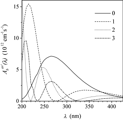
Figure 1: Spectral distribution of $a^{3}\Sigma_{g}^{+},v^{\prime}\to b^{3}\Sigma_{u}^{+}$ spontaneous emission transition probabilities for various initial vibronic levels $v^{\prime}=0-3$ (curves $0-3$) of the H₂ molecule [6, 7].

For H₂ molecule the values of $A_{b}^{av^{\prime}}(\lambda)$ should be considered as well-known nowadays because they have been calculated in several works [1, 5, 6, 7, 14] and checked experimentally [1, 4], being in rather good agreement [7]. We used the results of [6] shown in Table 1. In Fig. 1 the data are visualized for the transitions from $a^{3}\Sigma_{g}^{+},v^{\prime}$=0-3 levels for $\lambda=200-450$ nm. One may see that the probability of transitions from various vibronic levels has maxima in different wavelength regions due to oscillatory behavior of the vibrational wave functions of the upper state. So the spectral distribution of the continuum intensity $I_{ab}(\lambda)$ may have a certain informational content about the population density distribution over vibrational levels of the $a^{3}\Sigma_{g}^{+}$ electronic state. In principle, measurements of the intensity $I_{ab}(\lambda)$ may be used for the determination of the populations $N_{av^{\prime}}$ in relative or even in absolute scale by Eq. (1).

It should be noted that even this very first stage of the data processing belongs to the class of so-called reverse (or inversion) problems, which are known to be not well-posed (sometimes they are called “ill-posed”). The final result – a certain set of the populations $N_{av^{\prime}}$ – depends (in principle) not only on the values of the actual populations in plasma, but may be influenced by so-called a priory information: the number of adjusted parameters ($N_{av^{\prime}}$), the number of experimental data points, the experimental errors and even the algorithm of data processing.

In the present work we used for the solution of this and other reverse problems the least-square fitting, i.e., the minimization of the functional

$$\chi^{2}=\frac{1}{l-m}\ \sum\limits_{i=1}^{l}\left(\frac{Y_{i}^{\text{calc}}(a_{1},\dots,a_{m})-Y_{i}^{\text{expt}}}{\sigma_{i}}\right)^{2}\\$$ (3)

in the multidimensional space of parameters $a_{1},\dots,a_{m}$ used in a theoretical model. Here $Y_{i}^{\text{calc}}(a_{1},\dots,a_{m})$, $Y_{i}^{\text{expt.}}$ – calculated and experimental data, $l$ – total number of data points, $m$ – number of adjusted parameters, $\sigma_{i}$ – standard deviations of the experimental data. The standard deviations of optimal values of the adjusted parameters may be estimated as square roots of diagonal terms of the covariance matrix [29].

We used a minimization algorithm analogous to a linear regression [29] with the following substitutions: $Y_{i}^{\text{expt}}\equiv I_{ab}^{\text{expt}}(\lambda_{i})$ from experiment, $Y_{i}^{\text{calc}}\equiv I_{ab}(\lambda_{i})$ from Eq. (1), $\sigma_{i}\equiv 0.07\cdot I_{ab}^{\text{expt}}(\lambda_{i})$ corresponding to 7% random experimental error of the measurement, $m\equiv v^{\prime}_{\text{max}}+1$, $\lambda_{i}$ was varied in the range $225-400$ nm. Experimental errors were estimated by averaging of several measurements for the same conditions in plasma. They are mainly caused by random noise, non-sufficient stability of the discharges during the experiments and restricted reproducibility. The value of $v^{\prime}_{\text{max}}$ had to be adjusted in such a way that reliable results can be obtained from the minimization procedure. The values of $A_{b}^{av^{\prime}}(\lambda)$ from Table 1 were interpolated by cubic splines.

II.2 Excitation-deactivation balance equation

The populations of $N_{av^{\prime}}$ may be sometimes interesting themselves (see the examples below). But on the other hand, in non-equilibrium plasmas the rovibronic level populations in excited electronic states are connected with those in the ground electronic state by the excitation-deactivation balance equation for the electronically excited $n^{\prime},v^{\prime},N^{\prime}$ rovibronic levels [30]

$$\sum\limits_{vN}N_{XvN}\cdot n_{e}\cdot\alpha_{XvN}^{n^{\prime}v^{\prime}N^{\prime}}+I_{n^{\prime}v^{\prime}N^{\prime}}(\alpha,\beta,\gamma,\dots)=N_{n^{\prime}v^{\prime}N^{\prime}}\left(\frac{1}{\tau_{n^{\prime}v^{\prime}N^{\prime}}^{\text{rad}}}+\frac{1}{\tau_{n^{\prime}v^{\prime}N^{\prime}}^{\text{coll}}}\right),$$ (4)

where $I_{n^{\prime}v^{\prime}N^{\prime}}(\alpha,\beta,\gamma,\dots)$ – the rate of secondary excitation processes (cascades, recombination and so forth); $\tau_{n^{\prime}v^{\prime}N^{\prime}}^{\text{rad}}$ – radiative lifetime of the $n^{\prime}v^{\prime}N^{\prime}$ level; $\tau_{n^{\prime}v^{\prime}N^{\prime}}^{\text{coll}}$ – effective lifetime describing the decay of the $n^{\prime}v^{\prime}N^{\prime}$ level due to quenching in collisions of the excited molecule with electrons, atoms and unexcited molecules. The rate coefficient of direct electron impact excitation

$$\alpha_{XvN}^{n^{\prime}v^{\prime}N^{\prime}}=\langle\sigma{\mathbf{v}\rangle}_{XvN}^{n^{\prime}v^{\prime}N^{\prime}}=\int\nolimits_{\varepsilon_{th}}^{\infty}\sqrt{\frac{2\varepsilon}{m}}\ \sigma_{XvN}^{n^{\prime}v^{\prime}N^{\prime}}(\varepsilon)\ F(\varepsilon)\ d\varepsilon,$$ (5)

where $\sigma_{XvN}^{n^{\prime}v^{\prime}N^{\prime}}(\varepsilon)$ – corresponding cross section; $\mathbf{v},\varepsilon$ – velocity and corresponding energy of an incident electron; $\varepsilon_{th}$ – threshold energy of the $n^{\prime},v^{\prime},N^{\prime}\leftarrow X,v,N$ transition; $F(\varepsilon)$ – the electron energy distribution function.

For plasma diagnostics this most simple limit case (often called corona or corona-like model) is that of low-pressure plasmas with small input power. Under such conditions the levels are predominantly excited by direct electron impact excitation and their decay is mainly due to spontaneous emission. Than the second terms in right and left hand parts of Eq. (4) may be omitted.

It may be seen from Eqs. (2) and (3) that even in the most favorable case for plasma diagnostics the populations $N_{n^{\prime}v^{\prime}N^{\prime}}$ depend not only on the distribution $N_{XvN}$. Radiative transition probabilities, lifetimes and electron impact cross sections for single rovibronic levels and transitions should be known as well as the electron energy distribution function. Moreover the determination of $N_{XvN}$ from measured $N_{n^{\prime}v^{\prime}N^{\prime}}$ and with the certain system of equations (2) for various $v^{\prime}$ and $N^{\prime}$ lead to a reverse problem.

II.3 Constants of elementary processes

Further simplification of the model may be achieved by detailed analysis of radiative and collision transition probabilities and lifetimes. We are interested in determination of the vibrational temperature $T_{\text{vib}}$ from the continuum intensity ($a^{3}\Sigma_{g}^{+}\to b^{3}\Sigma_{u}^{+}$) and from the intensities of Q-branch lines of Fulcher-$\alpha$ bands ($d^{3}\Pi_{u}^{-}\to a^{3}\Sigma_{g}^{+}$). Therefore we have to analyze all available data about electron impact excitation and spontaneous decay of the upper levels.

The transition probabilities for $d^{3}\Pi_{u}^{-},v^{\prime},N^{\prime}$=1 $\to$ $a^{3}\Sigma_{g}^{+},v^{\prime\prime},N^{\prime\prime}$=1 transitions [Q1 lines of $(v^{\prime}-v^{\prime\prime})$ Fulcher-$\alpha$ bands] were obtained semi-empirically in the framework of the adiabatic approximation with corresponding dipole moment obtained in [33] from experimental data about wave numbers, branching ratios in $v^{\prime\prime}$-progressions and radiative lifetimes. The results for the first seven diagonal ($v^{\prime}$=$v^{\prime\prime}$=$v$) bands are presented in Table 2 together with semi-empirically predicted [33] and experimental values of radiative lifetimes [31].

One may see a noticeable discrepancy between semi-empirical and experimental lifetimes of $d^{3}\Pi_{u}^{-},v^{\prime}$=4-6, $N^{\prime}$=1 rovibronic levels due to non-adiabatic effects neglected in the adiabatic approximation (see also [10, 31]). Therefore, only the first four diagonal bands may be used for the determination of $T_{\text{vib}}$. On the other hand this effect did not influence the values of the rotational temperatures derived from the populations of $d^{3}\Pi_{u}^{-},v^{\prime}>$3 levels in [34]. It may be considered as an indication, that the rate of the additional decay, associated with a non-adiabatic coupling of the vibronic levels lying above the H($n$=1) + H($n$=2) dissociation limit, is almost independent on $N^{\prime}$ (here $n$ is the principle quantum number). It seems quite reasonable, if the perturbation is due to an electron-rotational interaction with a continuum (the hypothesis proposed in [35]). Because of the lack of information about $N^{\prime}$–dependences of the transition probabilities and the lifetimes they will be considered herein as independent on the rotational quantum number in accordance with an adiabatic approximation.

The radiative lifetimes of $a^{3}\Sigma_{g}^{+},v^{\prime}$ vibronic states of H₂ have been studied in numerous works both experimentally [2, 3, 12, 36, 37, 38] and by ab initio calculations [1, 5]. All available data are collected in Table 3. One may see, that:

• Nothing is known about $N^{\prime}$–dependences of the lifetimes, so we again have to assume independence on $N^{\prime}$.

• Experimental data are obtained only for low vibronic states.

• The experimental and calculated data are in very good accordance for $v^{\prime}=0-2$, but for higher $v^{\prime}$ only ab initio data are available.

To be in consistence with the transition probabilities listed in Table 1 we have used values of $\tau_{av^{\prime}}$ marked in Table 3 as “p.w.” – present work. The lifetimes for $v^{\prime}=0-2$ were obtained by the integration of the tabulated values of the transition probabilities from Table 1. The values labeled with an asterisk for $v^{\prime}=3-6$ were obtained by extrapolating the lifetimes with the help of a third order polynomial fit of the data from [5] and a constant factor obtained from the average value of the ratios with our values for $v^{\prime}=0-2$.

The dependences of $d^{3}\Pi_{u}^{-},v^{\prime},N^{\prime}\leftarrow X^{1}\Sigma_{g}^{+}$,0,$N$ electron impact excitation on the incident electron energy have been studied in [32, 39, 40]. They have a normal form for singlet-triplet transitions: a sharp increase from the threshold to the maximum and a rather sharp decrease for higher energies. The data of [32, 39] are in good accordance and in [41] they were used for the extraction of the cross sections for different $v^{\prime}$ from rate coefficients and $F(\varepsilon)$ measured in [9]. The relative cross sections $\sigma^{dv^{\prime}1}_{X01}/\sigma^{d21}_{X01}$ in maximum are shown in Table 4 together with corresponding ratios of the Franck-Condon factors calculated in [42]. One may see noticeable deviation of measured values from those calculated in the Franck-Condon approximation. In [32] this discrepancy was interpreted as an evidence of a remarkable dependence of the scattering amplitude on the internuclear distance (non-Franck-Condon effect). Later the data from [9] have been used for the determination of the complete set of the cross sections for various $v,v^{\prime}$ and $N,N^{\prime}$ [41].

It is important to take into account that the relative cross sections in [9, 32, 41] are based on radiative transition probabilities and lifetimes obtained in adiabatic approximation (almost the same as in Table 4). As we already mentioned above the lifetimes of $v^{\prime}=4-6$ are in contradiction with such extrapolation. New data about $\tau_{dv^{\prime}1}$ and $A^{dv^{\prime}1}_{av^{\prime\prime}1}$ from Table 2 should be used for the determination of the cross sections from the line intensities measured in [9]. We made the recalculation and got the data presented in the sixth column of Table 4. One may see that they are in rather good agreement with corresponding ratios of Franck-Condon factors. It means that the dependence of the scattering amplitude on the internuclear distance is negligible in the case of the $d^{3}\Pi_{u}^{-}\leftarrow X^{1}\Sigma_{g}^{+}$ electron impact excitation of H₂. This is in accordance with recent ab initio calculations [43].

Nothing is known, so far as we know, about the cross sections for the $a^{3}\Sigma_{g}^{+},v^{\prime},N^{\prime}\leftarrow X^{1}\Sigma_{g}^{+},v,N$ excitation. Therefore, for both $d^{3}\Pi_{u}^{-}\leftarrow X^{1}\Sigma_{g}^{+}$ and $a^{3}\Sigma_{g}^{+}\leftarrow X^{1}\Sigma_{g}^{+}$ transitions we assume that the rate coefficients of the electron impact excitation have non-zero values only for $N^{\prime}=N$ rovibronic transitions. They are considered as independent on $N$ and proportional to corresponding Franck-Condon factors, i.e.,

$$\alpha_{XvN}^{n^{\prime}v^{\prime}N^{\prime}} \approx \alpha_{Xv}^{n^{\prime}v^{\prime}}\propto Q_{Xv}^{n^{\prime}v^{\prime}},\qquad\mbox{when}\qquad\Delta N^{\prime}\equiv N^{\prime}-N=0$$ (6)

$$\mbox{and}\quad\alpha_{XvN}^{n^{\prime}v^{\prime}N^{\prime}} = 0\hskip 79.66771pt\mbox{for}\hskip 29.87538pt\Delta N^{\prime}\neq 0$$ (7)

thus neglecting the momentum transfer in electron impact excitation [32, 44] and the rather small dependence of the rate coefficients on $F(\varepsilon)$. We used the only values of Franck-Condon factors for $d^{3}\Pi_{u}^{-}\leftarrow X^{1}\Sigma_{g}^{+}$ and $a^{3}\Sigma_{g}^{+}\leftarrow X^{1}\Sigma_{g}^{+}$ transitions which had been calculated in [42] (Tables 5 and 6).

II.4 Determination of vibrational temperature

Vibrational and rotational energies are not well separated in the ground electronic state of H₂ because of the small mass of the nuclei. Just to have a certain ability to characterize the distribution over vibrational levels we introduce the vibrational temperature by

$$N_{Xv}=\sum\limits_{N}N_{XvN}=\sum\limits_{N}\frac{\mbox{[H${}_{2}$]}\cdot\exp{\Bigl{(}-\frac{\Delta E_{Xv}}{kT_{\text{vib}}}\Bigr{)}}\cdot(2N+1)\cdot\exp{\Bigl{(}-\frac{\Delta E_{XvN}}{kT}\Bigr{)}}}{\sum\limits_{v}\exp{\Bigl{(}-\frac{\Delta E_{Xv}}{kT_{\text{vib}}}\Bigr{)}}\ \sum\limits_{N}(2N+1)\cdot\exp{\Bigl{(}-\frac{\Delta E_{XvN}}{kT}\Bigr{)}}}=\mbox{[H${}_{2}$]}\cdot\frac{\exp{\Bigl{(}-\frac{\Delta E_{Xv}}{kT_{\text{vib}}}\Bigr{)}}}{{\mathcal{P}}(T_{\text{vib}})},$$ (8)

where [H₂] – total concentration of molecules, $\Delta E_{Xv}=E_{Xv0}-E_{X00}$, $\Delta E_{XvN}=E_{XvN}-E_{Xv0}$ – vibrational and rotational energy differences, $T_{\text{vib}}$ and $T$ – vibrational and translational temperatures, ${\mathcal{P}}(T_{\text{vib}})$ – the vibrational partition function. So we assume that in all vibrational levels of the $X^{1}\Sigma_{g}^{+}$ state the populations of the rotational levels are in Boltzmann equilibrium with the gas temperature $T$.

Taking into account all the assumptions discussed above, the balance equation (4) may be written for the populations of $d^{3}\Pi_{u}^{-},v^{\prime}$ vibronic states after summation over rotational levels in the following form

$$\frac{1}{{\mathcal{P}}(T_{\text{vib}})}\sum\limits_{v}Q_{Xv}^{dv^{\prime}}\cdot\exp{\left(-\frac{\Delta E_{Xv}}{kT_{\text{vib}}}\right)}\propto\frac{N_{dv^{\prime}}}{\tau_{dv^{\prime}}}.$$ (9)

One may see that the determination of $T_{\text{vib}}$ may be achieved by numerical solution of the system of equations (9) for several levels $v^{\prime}$ with experimental data about $N_{dv^{\prime}}$ derived from the intensities of the Fulcher-$\alpha$ Q-branch lines of diagonal ($v^{\prime}=v^{\prime\prime}$) bands:

$$N_{dv^{\prime}}=\sum\limits_{N}\frac{I_{av^{\prime}N}^{dv^{\prime}N}}{A_{av^{\prime}N}^{dv^{\prime}N}}.$$ (10)

This method of the $T_{\text{vib}}$ determination is based on sufficiently simple kinetics model and certain set of constants presented in Tables 2 and 6. It is even more simple then the predecessor [9] because it needs only intensity measurements.

In the framework of our model the continuum intensity can be written as

$$I_{ab}(\lambda,T_{\text{vib}})\propto\frac{1}{{\mathcal{P}}(T_{\text{vib}})}\sum\limits_{v^{\prime}}A_{b}^{av^{\prime}}(\lambda)\cdot\tau_{av^{\prime}}\cdot\sum\limits_{v=0}^{v^{\prime}_{\text{max}}}Q_{Xv}^{av^{\prime}}\cdot\exp{\left(-\frac{\Delta E_{Xv}}{kT_{\text{vib}}}\right)}.$$ (11)

To be able to work with relative intensities we may introduce the normalized relative intensity

$$J_{ab}(\lambda,\lambda_{0},T_{\text{vib}})=I_{ab}(\lambda,T_{\text{vib}})/I_{ab}(\lambda_{0},T_{\text{vib}}),$$ (12)

which is equal to unity for $\lambda=\lambda_{0}$.

The normalized intensities (12) may be tabulated for various values of $T_{\text{vib}}$ and then may be used for a determination of the vibrational temperature by least squares fitting (3) of experimental and calculated continuum intensity distributions. The results of our calculations for $\lambda_{0}=355.5$ nm and $T_{\text{vib}}$ = 0, 3000 and 5000 K are shown in Fig. 2. One may see that a variation of vibrational temperature leads to certain change in the shape of the continuum intensity distribution. Most sensitive are the wavelength regions near $\lambda\approx 200$ and 300 nm. The first one is out of our range of observation and cannot be used for diagnostics herein. Nevertheless the fact should be considered as one of the results of our present work. It may be recommended for VUV spectroscopy if the problems of the sensitivity calibration in this difficult region would be solved somehow (with the use of synchrotron radiation, for example). The changes near $\lambda\approx 300$ nm are less pronounced, therefore they may be used in the following way.

When the vibrational temperature is sufficiently low and

$$Q_{X0}^{av^{\prime}}\gg\sum\limits_{v=1}Q_{Xv}^{av^{\prime}}\cdot e^{-\frac{\Delta E_{Xv}}{kT_{\text{vib}}}},$$ (13)

then the excitation from vibronic levels with $v>0$ may be neglected and

$$J_{ab}(\lambda,\lambda_{0},0)=\frac{\sum\limits_{v^{\prime}=0}^{v^{\prime}_{\text{max}}}A_{b}^{av^{\prime}}(\lambda)\cdot\tau_{av^{\prime}}\cdot Q_{X0}^{av^{\prime}}}{\sum\limits_{v^{\prime}=0}^{v^{\prime}_{\text{max}}}A_{b}^{av^{\prime}}(\lambda_{0})\cdot\tau_{av^{\prime}}\cdot Q_{X0}^{av^{\prime}}}$$ (14)

represents the shape of the continuum for $T_{\text{vib}}\to 0$. It does not depend on discharge conditions and may be easily calculated because molecular constants in Eq. (14) are known. The results of such calculation for $\lambda_{0}=355.5$ nm and $v^{\prime}_{\text{max}}=6$ are presented in the last column of Table 1. One may see that in the wavelength range of observation, $\lambda=225-400$ nm, the continuum intensity shows monotonic increase towards short wavelengths.

The ratio

$$J^{\prime}_{ab}(\lambda,\lambda_{0},T_{\text{vib}})=J_{ab}(\lambda,\lambda_{0},T_{\text{vib}})/J_{ab}(\lambda,\lambda_{0},0)$$ (15)

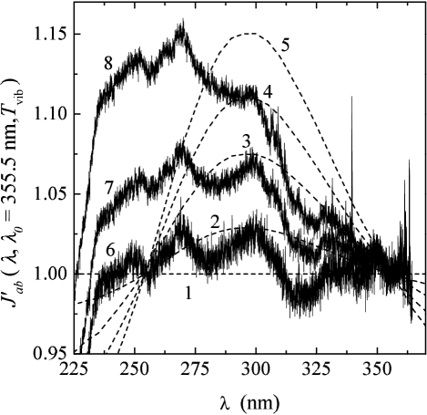
Figure 3: Normalized continuum intensity $J^{\prime}_{ab}(\lambda,\lambda_{0}\mbox{=355.5$\,$nm},T_{\text{vib}})$ calculated by Eq. (15) for various vibrational temperatures $T_{\text{vib}}$ = 0, 2000, 3000, 4000, 6000 K (curves 1, 2, 3, 4, and 5) and measured in capillary arc discharge at currents $i$ = 50, 200, and 300 mA (curves 6, 7, and 8).

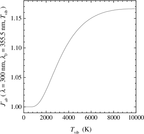
Figure 4: Normalized continuum intensity $J^{\prime}_{ab}(\lambda,\lambda_{0}\mbox{=355.5~{}nm},T_{\text{vib}})$ calculated for $\lambda=300$ nm as a function of the vibrational temperature $T_{\text{vib}}$.

may also be calculated for various values of the vibrational temperature and then be used as a nomogram for the determination of $T_{\text{vib}}$ from measured relative continuum intensity without solving the inverse problem by a minimization of Eq. (3). The results of such calculations for a limited number of $T_{\text{vib}}=0-6000$ K are shown in Fig. 3. One may see that the ratio (15) has some sensitivity to the vibrational temperature especially near 300 nm. For this particular wavelength we may organize a graph of $J^{\prime}_{ab}(\lambda=300\mbox{~{}nm},\lambda_{0}=355.5\mbox{~{}nm},T_{\text{vib}})$ versus $T_{\text{vib}}$ presented in Fig. 4 where the sensitivity is even more clear. This dependence may be used as a nomogram too, being especially useful for in situ control of plasmachemical processes.

III Experimental setup

As it was already mentioned in the introduction the experiments in pure hydrogen and H₂+Ar plasmas were carried out in two different gas discharges.

The first one is a hot cathode arc with 2 mm diameter constriction analogous to those used in [19, 20]. The discharge device was filled with 8 mbar of spectrally pure hydrogen. The range of the discharge current $I=10-500$ mA allowed us to achieve rather high current densities $j\approx 0.3-16$ A cm^-2.

The second plasma source was a H₂+Ar microwave discharge excited by a planar microwave applicator similar to that described in [24]. This plasma reactor has been specially designed for basic research on molecular microwave discharges mainly utilizing spectroscopic diagnostic methods [25]. The discharge configuration has the advantage of being well suited for end-on spectroscopic observations, because considerable homogeneity can be achieved to a certain extent, while side-on observations are also possible. Microwave plasma reactors of this planar type have been used for diamond deposition [26], surface corrosion protection by deposition of organo-silicon compounds [27] and surface cleaning [28]. The inner dimensions of the discharge vessel are 15$\times$21$\times$120 cm³ and the area of the quartz microwave windows was 8$\times$40 cm². The microwave power was fed in by a generator (SAIREM, GMP 12 KE/D, 2.45 GHz). We were able to measure the total input ($W=1.5$ kW) and reflected power, the latter was in our conditions always negligible ($<4$%). The input power flux in the plane of the applicator windows was roughly estimated to about 4 W cm^-2 assuming 20% heat loss to coolant and environment. The plasma length in end-on direction was $15\pm 3$ cm, mainly depending on the discharge pressure, and $8\pm 1$ cm in side-on observation, while for absorption spectroscopy the end-on direction was preferred. Gas flow controllers and a butterfly valve in the gas exhaust allow to have an independent control of gas inflow ($\varphi$ = 100 sccm) and pressure ($p=0.5-5$ mbar). The purity of gases was 99.996%. H₂ and Ar are used as components of the feed gas mixture, since they are not only of interest for basic research but of importance for various applications as well. Our main interests were focused on studies of: (1) influence of Ar on H₂ emission, and (2) dissociation of molecular hydrogen.

The central part of the plasma along the axis of the capillary discharge was focused by a quartz achromatic lens onto the entrance slit of a monochromator. In the microwave plasma the line of sight was 12 mm below the microwave windows of the applicator. For measurements of the continuum intensity we used a 0.5 m Czerny-Turner monochromator (Acton Research Corporation Spectra Pro–500) with gratings of 600 and 1200 grooves per mm in the first order. The line intensities of the Fulcher-$\alpha$ bands however were measured using a high resolution 1 m double monochromator of Czerny-Turner type with 1800 grooves per mm (Jobin Yvon RAMANOR U1000) in the first order. The output light was detected by a CCD matrix detector (TE-cooled, 512$\times$512 pixel, size of image zone: 9.7$\times$9.7 mm²) of the Optical Multichannel Analyzer PARC OMA IV connected with a computer. Special software made it possible to collect and analyze the recorded spectra.

The wavelength calibration was done by means of known Hg, Ar and H₂ spectral lines. The relative spectral sensitivity of the spectroscopic system in the range $\lambda=225-450$ nm has been obtained using a deuterium lamp (Heraeus Noble Light DO651MJ) calibrated by the Physikalisch–Technische Bundesanstalt (Braunschweig). The absolute value of the sensitivity for $\lambda=350$ nm was determined with a tungsten ribbon lamp. Its current-temperature calibration has been performed by the Russian State Institute of Standards (St.-Petersburg). We used two different currents corresponding to the absolute temperatures of tungsten $T$ = 2637 and 2763 K. This gave us usually a spread in the values of the sensitivity (at $\lambda=350$ nm) of less than 1%. The emissivity coefficient of the tungsten ribbon for these temperatures was taken from [47] and used for the calculation of the spectral distribution of emission intensity.

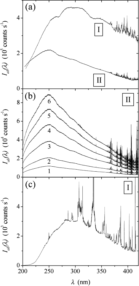
Figure 5: Experimental records (counts of CCD detector) of the continuum emission obtained in the dc capillary-arc discharges in (a) D₂, (b) H₂ with variation of the discharge current $i$ = 50, 100, 200, 300, 400, and 500 mA (curves 1, 2, 3, 4, 5, and 6) and (c) in the microwave discharge ($p=0.5$ mbar, H₂:Ar=1:1). Spectral distribution of the sensitivity is not taken into account. The measurements have been performed with gratings 600 (I) and 1200 (II) grooves per mm.

Some typical experimental records of the spectra of a standard deuterium lamp (a), pure hydrogen capillary-arc discharge (b) and H₂+Ar plasma of the microwave discharge (c) are presented in Fig. 5. The non-monotonic structure in the range $\lambda=250-350$ nm is connected with the spectral distribution of the sensitivity of our spectrometer. In the long-wavelength end of the first two records the band (actually multi-line) spectra of D₂ and H₂ molecules may be seen. One may see also that in spite of the gas flow mode our microwave plasma is not spectrally pure. It contains some impurities: oxygen (283 nm), OH-radical (bands at 283, $310-320$ nm), NH-radical (336 nm) and N₂ molecule (bands of the 2nd positive system $280-400$ nm mixed with H₂ bands). It should be noted that some lines are overexposed in the record shown in Fig. 5(c). The data of the continuum intensity, except those in Figs. 2, 3 and 5, were manually extracted from the measured intensity distribution.

As can be seen from previous description, the spectroscopic part of our experimental setup is certain combination of components commercially available nowadays. Therefore it may be easily reproduced. Experimental errors are mainly caused not by the detection system but by the random noise of plasma sources used. Special attention should be paid to selection of the continuum intensity from that of multi-line spectrum of H₂.

The results of our experiments will be presented together with corresponding analysis in the following sections. Perhaps most interesting of them are the first observations of: (1) small changes in the shape of the continuum in pure hydrogen plasma caused by vibrational excitation in the ground electronic state of H₂ molecule, (2) influence of Ar concentration on the shape of the continuum in H₂+Ar plasma of microwave discharge.

IV Results and Discussion

IV.1 Pure hydrogen dc capillary-arc discharge

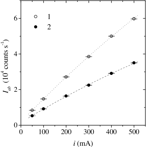
Figure 6: Signals of the continuum emission for $\lambda_{0}$ = 300 and 355.5 nm (points 1 and 2) against discharge current of H₂ capillary arc.

Relative intensities of the continuum and of the first Q-branch lines Q1 to Q5 of Fulcher-$\alpha$ bands ($v^{\prime}$=$v^{\prime\prime}$=0-5) were measured in the discharge current range mentioned above. The intensities were found to be proportional to discharge current if one takes into account a decrease of the density of molecules due to warming of the gas inside closed lamp by the hot cathode and discharge current. As an example the signals of CCD detector proportional to the continuum intensity are shown in Fig. 6 as a function of the discharge current. The linearity observed may be considered as an argument in favor of direct electron impact excitation of the levels under the study.

The shape of the continuum intensity distribution was observed to be independent on the discharge current for currents $i<100$ mA within experimental errors. A typical result used in further analysis is presented in Fig. 2. As one may see, measured continuum intensity is close to that calculated for $T_{\text{vib}}\to 0$. The low wavelength margin is limited by a sharp decrease of the sensitivity of our spectrometric system. For wavelengths longer than 360 nm the overlap of the continuum with band spectra of H₂ becomes more and more pronounced.

The first question to answer is how many populations of upper vibronic states can be obtained from the intensity distribution measured in the wavelength range of observation. To find the optimum number of adjusted parameters $N_{av^{\prime}}$ we made the $\chi^{2}$-minimization [Eq. (3)] with various $m=(v^{\prime}_{\text{max}}+1)$. The results of the calculations, made for the experimental data of Fig. 2, are presented in Table 7. $\chi^{2}$ shows a monotonic decrease and becomes lower than unity for $v^{\prime}_{\text{max}}\geq 3$. Another characteristic, presented in the table, is

$$\rho_{\text{max}}=\max{(\rho_{i})}\quad\mbox{with}\quad\rho_{i}=\sqrt{1-1/\Phi_{i}},$$ (16)

$$\mbox{where}\quad\Phi_{i}=Z_{ii}Z_{ii}^{-1}\quad\mbox{and}\quad Z_{lk}=\frac{\partial^{2}(\chi^{2})}{\partial a_{l}\partial a_{k}}.$$ (17)

The magnitudes $\rho_{i}$ are characteristics of the precision of the solution. Its zero value corresponds to the limit case of total independence of the parameters, while $\rho_{i}=1$ means that the parameter $a_{i}$ may be expressed as a linear combination of the other parameters and therefore the number of adjusted parameters should be decreased. It may be seen from Table 7 that in our case $\rho_{\text{max}}$ is growing with the increase of $m$; $\rho_{\text{max}}$ is close to unity for $v^{\prime}_{\text{max}}>$3. The maximum value of the relative standard deviation of the parameters $(\Delta N_{av^{\prime}}/N_{av^{\prime}})_{\text{max}}$ (in our case it is usually observed for $v^{\prime}$=$v^{\prime}_{\text{max}}$) is small and almost independent on $v^{\prime}_{\text{max}}$ for $v^{\prime}_{\text{max}}=0-3$, then it jumps to about 0.83 at $v^{\prime}=4$ and becomes much bigger for $v^{\prime}=5,6$. It means that the standard deviation of $N_{a4}$ derived from our spectrum is almost the same as its optimal value.

Thus in our case a determination of the populations of more than four vibronic levels is meaningless. The reason is very simple and may be seen from Table 8 where the relative populations $N_{av^{\prime}}/N_{a0}$ (obtained for $v^{\prime}_{\text{max}}=3$) are shown together with relative intensities of various $a^{3}\Sigma_{g}^{+},v^{\prime}\to b^{3}\Sigma_{u}^{+}$ transitions in the spectral range under the study ($\lambda=225-400$ nm)

$$\xi_{v^{\prime}}=\frac{\int\nolimits_{\lambda_{1}}^{\lambda_{2}}N_{av^{\prime}}\cdot A_{b}^{av^{\prime}}(\lambda)\,d\lambda}{\int\nolimits_{\lambda_{1}}^{\lambda_{2}}I_{ab}(\lambda)\,d\lambda}.$$ (18)

From the data of Table 8 it becomes clear that only 4% of the detected emission quanta originate from levels with $v^{\prime}>3$. The populations $N_{av^{\prime}}$ observed in the pure hydrogen capillary-arc discharge for currents $i=10-100$ mA are quite close to those calculated in the framework of our simple model with $T_{\text{vib}}\to 0$. It means that the populations of the $X^{1}\Sigma_{g}^{+},v$ vibronic levels with $v>0$ are so small that they do not affect relative populations of $a^{3}\Sigma_{g}^{+},v^{\prime}$ levels and therefore relative continuum intensity distribution.

For currents higher than $50-100$ mA we observed some systematic changes in the shape of the continuum intensity distributions. As an example our experimental data on the normalized intensities $J^{\prime}_{ab}(300,355.5,T_{\text{vib}})$ from Eq. (15) are presented for three values of the discharge current in Fig. 3 together with the curves calculated with our model for various values of $T_{\text{vib}}$. One may see that two main predictions of our model - the maxima near 300 nm and crossing with $J_{ab}^{\prime}=1$ near 250 nm - are in qualitatively good accordance with the experiment. The experimental curves are a bit shifted to shorter wavelengths. To treat the data quantitatively one should take into account that the differences between experimental and theoretical curves are comparable with errors of both the experiment and modeling:

1. The actual random noise of our measurements is about two times bigger than that shown in Fig. 3 due to smoothing during calibration procedure. It was made for better visibility of the trend.

2. The normalized intensity $J_{ab}^{\prime}$ is the ratio of the measured intensities, so its errors are twice more than that of measured intensities.

3. The systematic errors of the measurement may be even bigger because errors of the sensitivity calibration should be included, while the errors of the relative energy calibration of the deuterium lamp are about 4%.

4. Errors of the calculations are not so easy to estimate, but most likely they may be of the same order of magnitude. They are caused by the approximations made in the formulation of our very simple excitation-deactivation model [Eq. (4)] and by the uncertainties of the rate coefficients (see Section II.3).

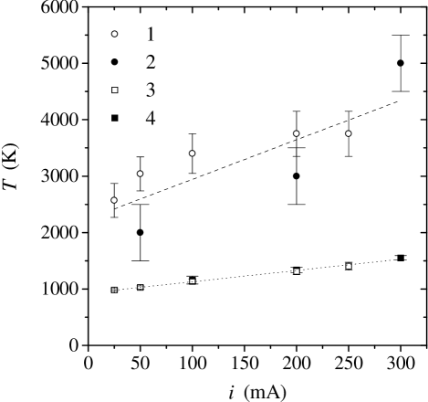
Figure 7: Vibrational (1,2) and rotational (3,4) temperatures in the ground $X^{1}\Sigma_{g}^{+}$ state of the H₂ in the capillary-arc pure hydrogen plasma for various discharge currents $i$ determined from the continuum intensity distribution (1) and from the emission of Fulcher-$\alpha$ bands (2-4). The data (1-3) – present work, (4) – Ref. [23].

Nevertheless, we used the values of maximum deviation of experimental curves from $J_{ab}^{\prime}=1$ level for estimation of $T_{\text{vib}}$. The results are shown in Fig. 7 together with values of $T_{\text{vib}}$ obtained from Fulcher-$\alpha$ band intensities by a system of Eqs. (9) for $v^{\prime}=0-3$. One may see that both spectroscopic methods of $T_{\text{vib}}$ determination developed in the present work are in good accordance.

The ground state rotational temperature was obtained from the intensity distributions in Fulcher-$\alpha$ Q branches by the method proposed in [48]. In our conditions the rotational and translational (gas) temperature are known to be in rather good accordance [22, 30, 34]. The results are also shown in Fig. 7 together with earlier data obtained in [23]. One may see that our measurements show remarkable difference between $T_{\text{vib}}$ and $T$ analogous to that observed in other conditions by CARS [49].

For currents higher than 300 mA the continuum intensity distribution became again insensitive to the current variation. This is most probably caused by large values of gas temperature and concentration of atomic hydrogen that is favorable for the acceleration of the VT-relaxation. On the other hand this behavior can also be explained by our model, since there is a certain upper limit above which the continuum intensity distribution is no longer sensitive to an increase of vibrational temperature (see Fig. 4).

IV.2 Microwave discharge in H₂+Ar mixture

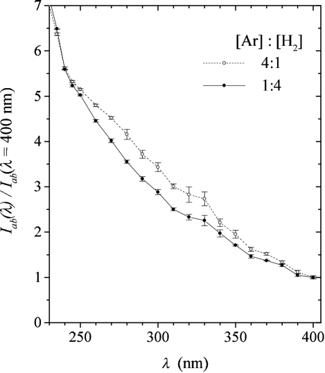
Figure 8: The relative continuum intensity (normalized for unity at $\lambda=400$ nm) measured in a H₂+Ar microwave plasma for two different ratios of the components at $p=0.5$ mbar.

The results of our measurements show that the spectral intensity distribution of the continuum in the H₂+Ar microwave discharge has a noticeably different shape compared to that in pure hydrogen. Moreover, the shape was found to depend on the ratio of the components in the mixture ([Ar]:[H₂]), which was varied from (19:1) to (1:4) under the same total pressure and power input. We observed a relative increase of the continuum emission in the wavelength region near 300 nm. As an illustration some typical results for (4:1) and (1:4) mixtures are shown in Fig. 8. One may see that the additional emission is located in the same wavelength interval as $a^{3}\Sigma_{g}^{+},v^{\prime}$=0$\to b^{3}\Sigma_{u}^{+}$ transition of H₂ (see Fig. 1) and ArH* (see below). Note that measurements in between exhibit a monotonic dependence of the increased emission in the wavelength range around 300 nm. An analysis of various possible explanations of the observed phenomenon lead us to the assumption that in our conditions an excitation transfer from excited Ar atoms to the hydrogen molecules might take place.

This experimental observation leads to two important consequences:

1. The shape of the continuum in H₂+Ar plasma is affected by two different excitation processes, therefore our model based on one of them (direct electron impact excitation) can not be used for the determination of $T_{\text{vib}}$.

2. To check the hypothesis of excitation transfer in our plasma we have to accompany our emission intensities with absorption measurements of populations of long-living states of Argon atoms (see Section IV.2.2).

IV.2.1 Ar*$\to$H₂ excitation transfer, prehistory

Excitation transfer in collisions of metastable (³P${}^{\circ}_{0,2}$) and resonant (³P${}^{\circ}_{1}$ and ¹P${}^{\circ}_{1}$) Ar atoms with hydrogen molecules is known since the pioneer work of Lyman [50] and was investigated so far in plasma and beam experiments mainly as: (1) quenching of excited Ar and (2) additional excitation of VUV Lyman and Werner bands ($B^{1}\Sigma_{u}^{+}$, $C^{1}\Pi_{u}$ $\to$ $X^{1}\Sigma_{g}^{+}$) of H₂. The first attempts to study the role of this effect in the emission of the hydrogen dissociation continuum in H₂+Ar plasmas appeared quite recently [22, 51, 52, 53].

The excitation of $a^{3}\Sigma_{g}^{+}$ state of H₂ due to the excitation transfer from excited Ar* atoms to the ground state H₂ molecule may go in two different ways:

$$\mbox{Ar${}^{*}$(4s${}^{1,3}$P${}^{\circ}_{J}$) + H${}_{2}$($X^{1}\Sigma_{g}^{+},v,N$) + $T_{0}$ \hskip 14.22636pt $\to$ \hskip 14.22636pt (ArH${}_{2}$)${}^{*}$}\hskip 14.22636pt\to$$ (19)

$$\hskip 5.69054pt\to\left\{\begin{array}[]{c}\mbox{H${}_{2}$*($a^{3}\Sigma_{g}^{+},v^{\prime},N^{\prime}$) + Ar(${}^{1}$S${}_{0}$) $\to$ 2 H($1^{2}$S${}_{1/2}$) + Ar(${}^{1}$S${}_{0}$)}+T_{1}+h\nu(\mbox{H${}_{2}$})\hskip 51.21495pt(\ref{eq:R2}a)\\[12.0pt] \mbox{ArH*($A^{2}\Sigma,v^{\prime},N^{\prime}$) + H($1^{2}$S${}_{1/2}$) $\to$ 2 H($1^{2}$S${}_{1/2}$) + Ar(${}^{1}$S${}_{0}$)}+T_{2}+h\nu(\mbox{ArH}).\hskip 31.29802pt(\ref{eq:R2}b)\end{array}\right.$$

Here (ArH₂)* denotes a temporary excited state of the system during the interaction, $T_{0}$ and $T_{1}$, $T_{2}$ are the initial and final kinetic energies of reacting particles in the mass center frame. The branching ratio between these two output channels of the reaction should depend on the initial excited state of the Ar atom and the vibro-rotational state of the molecule as well as on the collision energy $T_{0}$. As far as we know it is not established up to now in spite of a certain attempt in crossed beam experiments [4].

It may be shown, that if one wants to consider the excitation transfer possibility for ^1,3P${}^{\circ}_{J}$ argon atoms with various $J$ values from the energy point of view, the existence of vibro-rotational and translational energies of H₂ molecules in plasma should be taken into account [53]. Then in our conditions the observed effects are most likely due to the collisions of the resonant ³P${}^{\circ}_{1}$ and metastable ³P${}^{\circ}_{2}$ argon atoms with the $X^{1}\Sigma_{g}^{+},v$=0 hydrogen molecules.

IV.2.2 3s²3p⁵4s level populations of Ar

To clear up the situation we measured the population densities of the Ar 3s²3p⁵4s (³P${}^{\circ}_{0,1,2}$ and ¹P${}^{\circ}_{1}$) levels by an ordinary self-absorption method with one mirror behind the discharge vessel [54].

Neglecting Stark broadening of the spectral lines the population of the initial state of $k\leftarrow i$ absorption transition may be presented as

$$N_{i}=\sqrt{\frac{\pi}{4\ln{2}}}\ \frac{\Delta\nu_{D}}{f_{0}f_{ik}}\ \kappa_{0},$$ (20)

where

$$f_{0}=\frac{\pi e^{2}}{m_{e}c}=2.64\cdot 10^{-2}\ \mbox{cm}^{2}\ \mbox{s}^{-1},$$ (21)

$f_{ik}$ – the oscillator strength for the $k\leftarrow i$ transition in units of $f_{0}$, $\Delta\nu_{D}$ – the Doppler half-width depending on the gas temperature.

The absorption coefficient $\kappa_{0}$ was obtained by numerical solutions of the following non-linear equation [54]:

$$2\left[1-\frac{S(2\kappa_{0}l)}{S(\kappa_{0}l)}\right]=\frac{(1+r)-I_{m}/I_{0}}{r},$$ (22)

where $I_{m}$ and $I_{0}$ – the line intensities measured with and without the mirror, $l$ – length of plasma column along the axis of observation, $r$ – the reflection coefficient of the mirror and $S(x)$ – the Ladenburgh-Lévy function calculated by formulas from [55].

The effective reflection coefficient has been determined experimentally by the measurements of several Ar lines (603.1, 703.0, 714.7, 789.1, 860.6, 862.0, and 876.1 nm) which are free of self-absorption. It was found to be $r=0.52\pm 0.02$ and independent on $\lambda$. We used the values of the oscillator strengths from [56].

The intensities of two or three different spectral lines were used for the population density determination of every 3s²3p⁵4s level, namely:

1. – 763.511, 801.479, 811.531 nm

2. – 751.465, 738.398, 810.369 nm

3. – 794.815, 866.794 nm

4. – 826.452, 840.821 nm.

The conditions were the same as those used in our measurements of the continuum intensity.

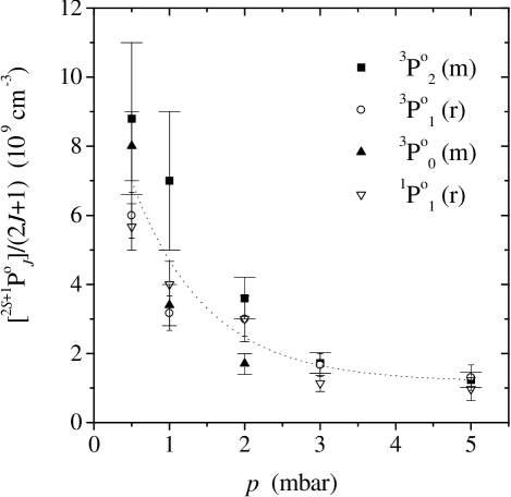
Figure 9: The scaled population densities of ^1,3P${}^{\circ}_{J}$ levels of Ar as a function of total pressure $p$ for constant gas mixture H₂+Ar (1:1) in the microwave discharge plasma. The total average population of all 3s²3p⁵4s levels may be obtained by multiplication of 12 to the dashed curve.

Typical results are shown in Fig. 9. The scaled populations are absolute values of the level population densities divided by their statistical weights $(2J+1)$. They have the meaning of the average populations of the multiplet structure sublevels. In equilibrium conditions they should be almost equal to each other because the levels have almost the same energy – 11.55, 11.62, 11.72, and 11.83 eV for ³P${}^{\circ}_{2}$, ³P${}^{\circ}_{1}$, ³P${}^{\circ}_{0}$, and ¹P${}^{\circ}_{1}$. One may see from Fig. 9 that in our conditions:

1. The populations of various sublevels of all resonant and metastable states coincide within the experimental errors. It is a direct manifestation of long effective lifetimes of the resonant levels (due to self-absorption of the resonant radiation) and a high enough rate of collisional transitions between the 3s²3p⁵4s levels. So the metastable and resonant levels of Ar are actually mixed in the plasma under the study.

2. The sublevel populations show the monotonic decrease with total pressure which may be connected with: a decrease of microwave power applied to plasma in the volume of observation, a decrease in the rate coefficient of electron impact excitation (due to certain changes of electron velocity distribution) and an increase of collisional quenching.

3. The total population of all 12 sublevels may reach $10^{11}$ cm^-3 at low pressures. The rate coefficients of the Ar*$\to$H₂ excitation transfer are approximately $10^{-10}$ cm³ s^-1 [16]. Thus the rate of the continuum excitation in the reaction is about 10¹⁶ cm^-3 s^-1. This is comparable with the observed total continuum emission (see Table 9) and should be taken into account together with direct electron impact excitation of the $a^{3}\Sigma_{g}^{+}$ state of H₂.

IV.2.3 Shape of the continuum in H₂+Ar plasma

Let us assume the spectral distribution of the continuum intensity as the sum of three independent terms corresponding to three different excitation mechanisms:

$$I_{ab}^{\text{calc}}(\lambda)=A[c_{1}I_{ab}(\lambda,0)+c_{2}I_{b}^{a0}(\lambda)+c_{3}I_{\text{ArH}}(\lambda)],$$ (23)

where $A$ – absolute scale normalization constant equal to total continuum intensity in the range of observation $\lambda=225-400$ nm, $I_{ab}(\lambda,0)$ – spectral distribution of the continuum radiation caused by the electron impact excitation of H₂ from lowest $X^{1}\Sigma_{g}^{+},v$=0 vibronic ground state [Eq. (14)], $I_{b}^{a0}(\lambda)$ – the same due to the reaction (19a) for $v^{\prime}=0$ only, $I_{\text{ArH}}(\lambda)$ – the spectral distribution corresponding to the reaction (19b) calculated in [4], $c_{i}$ – the coefficients representing relative contributions of the components ($\sum_{i}c_{i}=1$). The spectral distributions $I_{ab}(\lambda,0)$, $I_{b}^{a0}(\lambda)$ and $I_{\text{ArH}}(\lambda)$ where normalized for unit area in the range of wavelengths $\lambda=225-400$ nm.

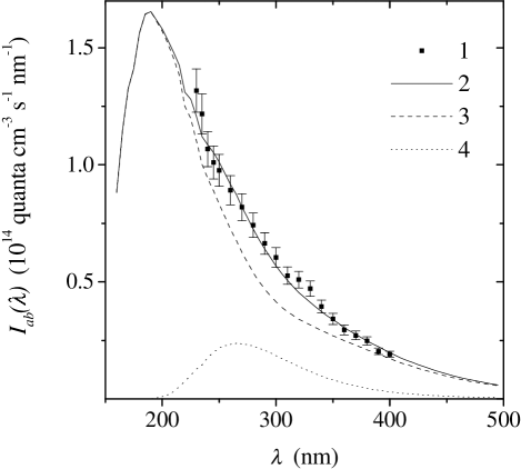
Figure 10: Spectral distribution of the continuum emission in the H₂+Ar (1:1) microwave plasma for the total pressure $p$ = 0.5 mbar. 1 – experimental data points, 2 – calculated by Eq. (23) with the optimal set of parameters $A,c_{1},c_{2},c_{3}$ shown in Table 9, 3 – the contribution of the electron impact excitation for $T_{\text{vib}}\to 0$ with $v^{\prime}_{\text{max}}$=3, 4 – contribution of the Ar*$\to$H₂ excitation transfer to $a^{3}\Sigma_{g}^{+},v^{\prime}$=0.

Then the spectral distributions of the continuum measured in the microwave plasma under various conditions were fitted by the function (23) according to Eq. (3). Typical results are presented in Table 9 for five selected mixtures of Ar+H₂ from (1:4) up to (19:1). The first set of $\chi^{2}$-minimizations marked as ($c_{1},c_{2},c_{3}\neq 0$) was made without any additional preconditions. One may see that the observed shape of the continuum may be described by three adjusted parameters of the expansion (23) with rather good precision ($\chi^{2}=1-2$). Moreover the fittings show the negligible contribution of the reaction (19b), which cannot be considered as significant because the values of $c_{3}$ are comparable with standard deviations of their determination. Figure 10 illustrates typical results of such fitting. The contribution of the reaction (19b) is too small to be visible in the figure.

The second set of fittings has been performed under the additional condition $c_{3}=0$. This version of the model provides almost the same precision in the description of the observed spectra taking into account only the first two mechanisms included into Eq. (23).

In contrast the third set of fittings has been carried out for $c_{2}=0$ thus neglecting a contribution of the reaction (19a). Again we got almost the same quality of fitting. These results are the direct consequence of the similarity of spectral distributions of the continuum emission caused by the reactions (19a) for $v^{\prime}=0$ and (19b).

It should be noted, that ab initio potential curves of ArH* where never checked experimentally and the spectral distribution of the ArH continuum has been calculated in [4] in the rough approximation of harmonic oscillator. The precision of such calculations cannot be high nowadays. Taking this into account we may assume that the insignificant contribution of the reaction (19b) obtained in the first set of fittings is an accidental numerical result. Most probably it is without any physical meaning because two other sets [based on directly opposite assumptions about the branching ratio between reactions (19a) and (19b)] gave us almost the same $\chi^{2}$ values.

Therefore, we have to conclude that the precision and the wavelength range of our measurements together with the lack of dependable ArH* transition probabilities do not allow us to distinguish contributions of the reactions (19a) and (19b). On the other hand, there is no doubt that in our conditions the role of the Ar*$\to$H₂ excitation transfer is well noticeable (10-30%) both in excitation and dissociation rates (see below).

IV.3 Estimation of the rate of electron impact dissociation

As it was already mentioned in the introduction, the absolute value of the intensity of the continuum is directly connected with the rate of the radiative dissociation via spontaneous emission to the repulsive $b^{3}\Sigma_{u}^{+}$ state. If self-absorption in the plasma volume may be neglected, then the rate of radiative dissociation due to $a^{3}\Sigma_{g}^{+}\to b^{3}\Sigma_{u}^{+}$ transitions is equal to the total continuum intensity (expressed in number of photons per cm³ in a second) integrated over the entire wavelength range

$$\left(\frac{d[\mbox{H${}_{2}$}]}{dt}\right)_{ab}=\int\nolimits_{0}^{\infty}I_{ab}(\lambda)d\lambda=\sum\limits_{v^{\prime}=0}^{v^{\prime}_{\text{max}}}\frac{N_{av^{\prime}}}{\tau_{av^{\prime}}}.$$ (24)

The wavelength range where we were able to measure the intensity was limited (see Fig. 2, 5, 8). So we detected only a part of the continuum emission. The rest should be obtained by some extrapolation. In pure hydrogen discharge plasma the vibrational temperature is usually rather low and the Eqs. (1) and (12) may be used for the extrapolation. The calculations show that in our case: (1) The dependence of the total intensity (area under the curve) on the $v^{\prime}_{\text{max}}$ is insignificant after $v^{\prime}_{\text{max}}$ became high enough. (2) The contribution of the undetected part of the spectrum is rather significant (about 60% in the example shown in Fig. 3).

The other, more general way of treating of spectroscopic data is a numerical solution of the reverse problem by $\chi^{2}$-minimization (3). The relative or absolute populations $N_{av^{\prime}}$ thus obtained may be used for the determination of the relative or absolute radiative dissociation rate. Radiative lifetimes are known, so an integration over wavelengths is not necessary and the procedure is reduced to only few summations in Eq. (24).

In low-pressure gas discharges the upper levels of the continuum transition are predominantly populated by $a^{3}\Sigma_{g}^{+}\leftarrow X^{1}\Sigma_{g}^{+}$ electron impact excitation [9, 10]. A dissociation of hydrogen molecules is also mainly caused by electron impact excitation of various intermediate excited electronic states, bound and repulsive ones. The relative contribution of various channels to the total electron impact dissociation cross section $\sigma_{\text{diss}}(\varepsilon)$ was analyzed in [57], later supplemented with an application of the close-coupling calculations of the cross-sections [58]. It was found that singlet-triplet transitions play the major role, $b^{3}\Sigma_{u}^{+}\leftarrow X^{1}\Sigma_{g}^{+}$ and $a^{3}\Sigma_{g}^{+}\leftarrow X^{1}\Sigma_{g}^{+}$ being most prominent. The experimental data for $\sigma_{\text{diss}}(\varepsilon)$ are available from [59].

All these cross-sections seem to have a rather similar shape as a function of the collision energy $\varepsilon$, except in the small region near the threshold, because an excitation of various electronic states obviously has different start-up energies. In [22] we proposed to use average values of ratios between the cross sections (determined far enough from threshold region) for the estimation of the rate of the radiationless $b^{3}\Sigma_{u}^{+}\leftarrow X^{1}\Sigma_{g}^{+}$ process $(d[\mbox{H${}_{2}$}]/dt)_{b\leftarrow X}$ and of the total dissociation rate $(d[\mbox{H${}_{2}$}]/dt)_{\text{diss}}$ by the multiplication of the measured total continuum intensity with certain coefficients (4 and 15 correspondingly). Actually, the coefficients depend on the shape of the electron energy distribution function and the total electron impact dissociation rate

$$\left(\frac{d[\mbox{H${}_{2}$}]}{dt}\right)_{\text{diss}}=\frac{\alpha_{\text{diss}}}{\alpha_{a\leftarrow X}}\left(\frac{d[\mbox{H${}_{2}$}]}{dt}\right)_{ab}.$$ (25)

Generally, the rate coefficients in (25) should be calculated with actual $F(\varepsilon)$ by Eq. (5) [9, 10]. If the distribution function is not available like in our present study, only rough estimations are possible. It is quite obvious that, when $\varepsilon$-dependences of the cross-sections have similar shapes, the ratio of the rate coefficients is less sensitive to the near-threshold region for $F(\varepsilon)$ with a high content of fast enough electrons. To check the tendency we calculated the ratios for a Maxwellian distribution with an electron temperature of $T_{e}=1-10$ eV and the cross sections from [58, 59]. The results are presented in Fig. 11. One may see that both ratios show sharp decrease for $T_{e}<5$ eV becoming almost independent from $T_{e}$ for $T_{e}>5$ eV. It is quite typical for a low-pressure hydrogen discharge plasma to have a strongly non-Maxwellian $F(\varepsilon)$ with a high density of fast electrons having energies sufficiently higher than the thresholds (see i.e. [60]). So we may use the asymptotes of Fig. 11 for the estimations. Numerical values of the coefficients are

$$\frac{\alpha_{b\leftarrow X}}{\alpha_{a\leftarrow X}}\sim 4.9\qquad\mbox{and}\qquad\frac{\alpha_{\text{diss}}}{\alpha_{a\leftarrow X}}\sim 16.$$ (26)

In the pure hydrogen capillary-arc discharge we were not able to carry out absolute measurements because the plasma is inhomogeneous along the axis of observation and the effective length of the emitting plasma column is uncertain [60].

However, in the H₂+Ar microwave plasma the length of emitting column ($8\pm 1$) cm is well defined and absolute continuum intensities were measured in a certain range of discharge conditions. But the Eqs. (24) and (26) are not valid any more, because Ar*$\to$H₂ excitation transfer plays an important role. The continuum intensity may be expressed as (23) and the total dissociation rate is a sum of the terms corresponding to the electron impact and the excitation transfer. It can be shown that in this case the total dissociation rate

$$\left(\frac{d[\mbox{H${}_{2}$}]}{dt}\right)_{\text{total}} = \left(\frac{d[\mbox{H${}_{2}$}]}{dt}\right)_{\text{diss}}+\left(\frac{d[\mbox{H${}_{2}$}]}{dt}\right)_{\text{Ar*}}$$ (27)

$$= A\left[\frac{\alpha_{\text{diss}}}{\alpha_{a\leftarrow X}}\,c_{1}\int\nolimits_{0}^{\infty}I_{ab}(\lambda,0)\,d\lambda+c_{2}\int\nolimits_{0}^{\infty}I_{b}^{a0}(\lambda)\,d\lambda+c_{3}\int\nolimits_{0}^{\infty}I_{\text{ArH}}(\lambda)\,d\lambda\right].$$ (28)

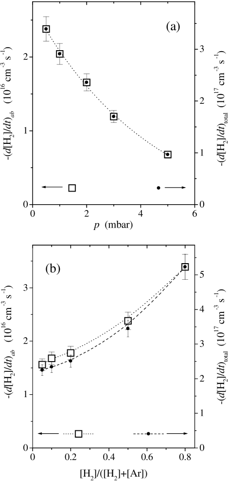
Figure 12: Radiative dissociation rate $(d[\mbox{H${}_{2}$}]/dt)_{ab}$ ($\Box$) and total electron impact dissociation rate $(d[\mbox{H${}_{2}$}]/dt)_{\text{total}}$ ($\bullet$) obtained in the H₂+Ar microwave discharge: (a) as a function of the total pressure $p$ for constant gas mixture (1:1) and (b) for various gas mixtures under constant total pressure $p$ = 0.5 mbar.

Spectral distributions of the intensities in the second and third terms are mainly located in the wavelength range of our observations (about 90%). Only the first one, connected with $a^{3}\Sigma_{g}^{+},v^{\prime}\leftarrow X^{1}\Sigma_{g}^{+},v$=0 excitation needs the extrapolation described above. Therefore, the total dissociation rate in our conditions may be calculated from the measured continuum intensity. The results are shown in Fig. 12(a,b) for various pressures and ratios of the components in the mixture. They may be interpreted only qualitatively.

Figure 12(a) shows that the dissociation rate in the volume of observation monotonically decreases with increasing pressure. The effect is analogous to that of the excited argon populations (see Fig. 9 and corresponding discussion). It is caused by the mechanisms already mentioned above, mainly by the decrease of microwave power coming to the volume of observation.

The observed changes in the dissociation rate caused by the variation of mixture components under constant pressure [Fig. 12(b)] are not trivial. In the absence of secondary effects one should expect linear dependence, whereas our measurements show a non-linear decrease of $(d[\mbox{H${}_{2}$}]/dt)_{\text{diss}}$ towards smaller values of [H₂]. Most probably the effect is connected with very simple reasons, which can be of importance for industrial systems. When the content of hydrogen in the input gas mixture is high enough, the concentration of hydrogen in plasma is proportional to that in the input gas mixture. If the hydrogen content in the feed gas is reduced, then the hydrogen density in plasma is mainly influenced by resorption of hydrogen and water from the rather large metal surfaces. If it would be necessary to achieve small concentrations of hydrogen in plasma, then heating and pumping of the reactor must be done for a very long time.

On the other hand the data presented in Fig. 12(b) show that in our conditions the Ar*$\to$H₂ excitation transfer plays noticeable role even in the total rate of hydrogen dissociation. This effect should be taken into account in kinetics modeling of atomic hydrogen concentration in plasmachemical systems where Ar is used for transportation of reagents as a buffer. Our observation shows that it is not just a buffer.

V Conclusion

In this paper for the first time the H₂ radiative dissociation continuum was used as a source of information about parameters of non-equilibrium plasma. Two new methods of spectroscopic diagnostics of hydrogen containing plasma have been developed: (1) determination of the vibrational temperature of the H₂ ground state from the relative intensity distribution and (2) derivation of the rate of electron impact dissociation from the absolute intensity of the continuum. The development of these methods has been based on a detailed analysis of the excitation-deactivation kinetics, rate constants of various collisional and radiative transitions as well as the way of data processing. The known method of vibrational temperature determination [9] using H₂ emission line intensities of Fulcher-$\alpha$ bands was significantly improved and simplified. The potential of the new methods for plasma diagnostics was demonstrated at pure H₂ capillary-arc and H₂+Ar microwave discharges.

In pure hydrogen discharge plasma it was observed for the first time that for high enough current densities $j\geq 3$ A cm^-2 the shape of the continuum intensity distribution is influenced by the vibrational temperature of the ground $X^{1}\Sigma_{g}^{+}$ electronic state. Two independent spectroscopic methods gave almost the same values of $T_{\text{vib}}\approx 2000-5000$ K. The difference between vibrational and gas temperatures is in accordance with previous observations [49].

In the H₂+Ar microwave plasma for the first time the shape of the H₂ dissociation continuum was found to depend on the mixture components, significantly influenced by Ar${}^{*}\to$H₂ excitation transfer processes. Absorption measurements of the population of the 3s²3p⁵4s levels of Ar together with certain computer simulation has been successfully used for verification of the proposed mechanism. Also for the first time the rates of radiative and total electron impact dissociation were obtained for various gas pressures and relative concentrations of the mixture components.

Our attempt to study the informational content of the intensity of the hydrogen dissociation continuum and to check its applicability for plasma diagnostics has been a priory limited in two different respects.

1) We intended to have an experimental technique as simple as possible and, in particular, to stay on the basis of emission spectroscopy only. Then the methods would be especially useful in various industrial applications including rather easy in situ control of plasma processing. The approach has in principle a backside because the knowledge of the actual electron energy distribution function and its spatial distribution may be of importance for a correct extraction of the information about plasma parameters. Langmuir probe measurements of electron energy distributions are not a problem nowadays, even in the cases of space-charge layers [60], RF [62, 63] and microwave discharges (see [64] and Refs. therein). We limited ourselves with intensity measurements in the more or less easy detectable near-UV region because the following second restriction of our attempt seems to be more significant.

2) Our analysis of the known characteristics of radiative and collisional processes involved into the mechanism of formation of observable continuum emission led us to the conclusion that in spite of numerous efforts the situation is still unsatisfactory. Therefore, only simple models can be used. The corona-like model of the excitation, neglecting the rotational structure of upper vibronic levels, and the Franck-Condon approximation for electron impact excitation are actually available and justified right now.

Nevertheless, even in such complicated conditions we were happy to find that more or less accurate measurements of relative and absolute spectral distributions of the continuum intensity may be used for certain estimations of the vibrational temperature, for the analysis of the excitation mechanisms and for getting information about the rate of hydrogen dissociation by electron impact.

The last one looks more prospective because in some cases it can be already used as it is. If, for example, one is interested in the relative dependence of the electron impact dissociation rate on the position in plasma or on the discharge conditions, the information may be easily obtained just by a measurement of the continuum emission intensity even without any calibrations. The method of the determination of the absolute rate of the electron impact dissociation may be considerably improved, if the electron energy distribution function would be determined experimentally or calculated somehow. Then there would be no need to use our graph in Fig. 11 but to calculate the values in an explicit way by Eq. (5).

This rather easy and independent method of determination of the absolute values of the rate of electron impact dissociation of hydrogen may be used in gas discharge physics and in plasma chemistry within two approaches.

1) It may be used for the determination of the hydrogen dissociation degree (which is often considered as a very important plasma parameter), if one is able to determine the effective mean lifetime of atoms in plasma with certain theoretical model of diffusion and association of atoms (see e.g. [65]).

2) If the value of the dissociation degree is determined by one of the existing methods (see [66, 67]) then the effective lifetime of atoms in plasma may be determined with the help of the rate of dissociation and the corresponding balance equation for atoms.

In both cases the method proposed in the present work is giving new opportunities.

Further improvements of the methods developed in present work need more detailed information about the elementary processes especially those about the cross sections of electronic-vibrational (better electronic-vibro-rotational) $a^{3}\Sigma_{g}^{+},v^{\prime},N^{\prime}\leftarrow X^{1}\Sigma_{g}^{+},v,N$ electron impact excitation and the rate coefficients of the quenching of $a^{3}\Sigma_{g}^{+},v^{\prime},N^{\prime}$ levels in collisions with electrons, atoms and molecules. We certainly understand those are not simple problems, but we may hope that the needs of plasma diagnostics and our present work may be considered as some kind of the challenge for our colleagues working in the field of electronic and atomic collision physics.

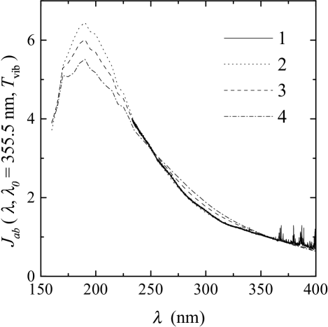
Figure 2: Relative distributions of the continuum intensity measured in the capillary-arc discharge with $I=100$ mA (curve 1) and those calculated for $T_{\text{vib}}$=0, 3000, 5000 K (curves 2, 3, and 4).

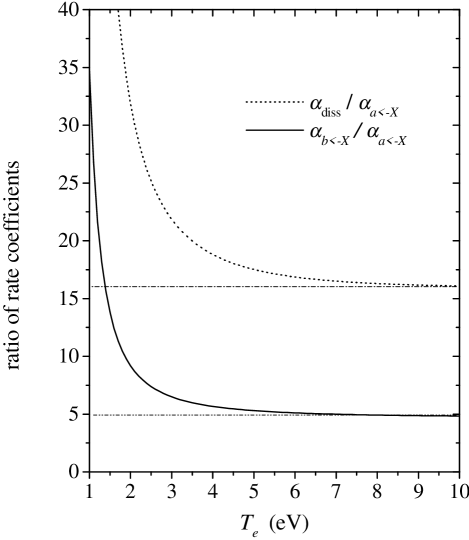
Figure 11: Ratios of the rate coefficients of electron impact excitation of $b^{3}\Sigma_{u}^{+}$ ($\alpha_{b\leftarrow X}$), $a^{3}\Sigma_{g}^{+}$ ($\alpha_{a\leftarrow X}$) states and of the total electron impact dissociation ($\alpha_{\text{diss}}$) calculated as a function of the electron temperature.

Table 1: Spectral distributions of transition probability for $a^{3}\Sigma_{g}^{+},v^{\prime}$=0-6$\to b^{3}\Sigma_{u}^{+}$ spontaneous emission of the H₂ molecule and relative continuum intensity calculated for $T_{\text{vib}}\to 0$ by Eq. (14).

$\lambda$	$A_{b}^{av^{\prime}}(\lambda)$ (1012 cm-1 s-1)     [6]							$J_{ab}(\lambda,355.5,0)$
[nm]	$v^{\prime}=0$	$1$	$2$	$3$	$4$	$5$	$v^{\prime}=6$	present work
160	$0$	$0$	$0$	$3.220$	$49.674$	$3.795$	$22.977$	3.717
170	$0$	$0$	$1.714$	$34.647$	$9.474$	$23.008$	$14.436$	5.339
180	$0$	$0.395$	$16.152$	$24.766$	$11.127$	$0.144$	$2.297$	6.034
190	$0$	$3.701$	$26.715$	$0.231$	$10.235$	$10.524$	$5.725$	6.454
200	$0.283$	$9.938$	$17.191$	$6.123$	$0.047$	$2.873$	$5.463$	6.147
210	$0.949$	$14.879$	$3.565$	$9.571$	$4.340$	$0.697$	$0.077$	5.590
220	$2.252$	$14.894$	$0.016$	$2.799$	$6.257$	$4.182$	$1.898$	4.829
230	$3.851$	$11.283$	$2.370$	$0.377$	$3.070$	$4.066$	$3.662$	4.300
240	$5.315$	$6.723$	$4.702$	$0.386$	$0.386$	$1.681$	$2.498$	3.666
250	$6.540$	$3.087$	$5.315$	$1.871$	$0.164$	$0.135$	$0.704$	3.218
260	$7.025$	$0.948$	$4.222$	$3.010$	$1.154$	$0.165$	$0.025$	2.788
270	$7.090$	$0.085$	$2.645$	$3.056$	$1.971$	$0.851$	$0.262$	2.407
280	$6.792$	$0.049$	$1.330$	$2.440$	$2.176$	$1.416$	$0.797$	2.089
290	$6.249$	$0.389$	$0.463$	$1.598$	$1.918$	$1.609$	$1.161$	1.822
300	$5.582$	$0.819$	$0.079$	$0.893$	$1.414$	$1.456$	$1.256$	1.616
310	$4.867$	$1.224$	$0$	$0.367$	$0.869$	$1.126$	$1.118$	1.451
320	$4.165$	$1.509$	$0.108$	$0.101$	$0.471$	$0.755$	$0.866$	1.325
330	$3.530$	$1.671$	$0.295$	$0.006$	$0.197$	$0.451$	$0.597$	1.222
340	$2.946$	$1.748$	$0.474$	$0.020$	$0.045$	$0.226$	$0.372$	1.130
350	$2.453$	$1.717$	$0.618$	$0.100$	$0.005$	$0.080$	$0.193$	1.042
360	$2.021$	$1.647$	$0.695$	$0.202$	$0.011$	$0.018$	$0.083$	0.955
370	$1.667$	$1.530$	$0.818$	$0.296$	$0.058$	$0.002$	$0.024$	0.885
380	$1.373$	$1.399$	$0.846$	$0.379$	$0.117$	$0.016$	$0.004$	0.809
390	$1.125$	$1.265$	$0.844$	$0.445$	$0.179$	$0.047$	$0.007$	0.736
400	$0.921$	$1.127$	$0.818$	$0.486$	$0.228$	$0.088$	$0.026$	0.665
410	$0.735$	$0.985$	$0.781$	$0.499$	$0.271$	$0.127$	$0.051$	0.592
420	$0.621$	$0.865$	$0.729$	$0.504$	$0.303$	$0.161$	$0.080$	0.534
430	$0.514$	$0.752$	$0.674$	$0.497$	$0.320$	$0.190$	$0.104$	0.477
440	$0.423$	$0.654$	$0.615$	$0.477$	$0.327$	$0.207$	$0.127$	0.424
450	$0.343$	$0.567$	$0.559$	$0.455$	$0.327$	$0.221$	$0.144$	0.376
460	$0.283$	$0.488$	$0.503$	$0.429$	$0.322$	$0.226$	$0.157$	0.333
470	$0.241$	$0.420$	$0.452$	$0.397$	$0.310$	$0.229$	$0.164$	0.295
480	$0.203$	$0.363$	$0.402$	$0.366$	$0.297$	$0.229$	$0.168$	0.261
490	$0.169$	$0.312$	$0.359$	$0.337$	$0.281$	$0.221$	$0.168$	0.231

Table 2: Radiative lifetimes of $d^{3}\Pi_{u}^{-},v,N$=1 levels and spontaneous emission transition probabilities of $d^{3}\Pi_{u}^{-},v,N$=1 $\to$ $a^{3}\Sigma_{g}^{+},v,N$=1 spectral lines of H₂.

	$\tau_{dv1}$ (ns)				$A^{dv1}_{av1}$ ($\mu$s-1)
$v$	[31, 34]		present work		present work
0	40.7${}\pm{}$	1.4	38.7${}\pm{}$	2.0	24.4${}\pm{}$	1.4
1	38.4${}\pm{}$	1.3	39.7${}\pm{}$	2.1	20.6${}\pm{}$	1.1
2	39.5${}\pm{}$	1.9	40.9${}\pm{}$	2.2	16.9${}\pm{}$	1.0
3	39.5${}\pm{}$	0.9	42.2${}\pm{}$	2.2	13.6${}\pm{}$	0.8
4	19.0${}\pm{}$	1.0	43.6${}\pm{}$	2.4	10.6${}\pm{}$	0.6
5	15.2${}\pm{}$	1.2	45.5${}\pm{}$	2.5	8.1${}\pm{}$	0.5
6	16.0${}\pm{}$	3.0	—		5.9${}\pm{}$	0.4

Table 3: Experimental and ab initio data on the radiative lifetimes of $a^{3}\Sigma_{g}^{+},v^{\prime}$ levels of H₂, p. w. - present work.

$\tau_{av^{\prime}}$ (ns)
$v^{\prime}$=0		1		2	$3$	$4$	$5$	$v^{\prime}=6$	Ref.
calculated
11.9		11.0		10.1	$9.7$	$---$	$---$	$---$	[1]
11.6		10.2		9.17	$8.40$	$7.81$	$7.30$	$6.90$	[5]
12.4		11.5		10.3	$9.29$	$8.64$	$8.07$	$7.63$	p.w.
experimental
35$\pm$8									[2]
11.0${}\pm{}$	0.42	10.6${}\pm{}$	0.6	—	$---$	$---$	$---$	$---$	[36]
26${}\pm{}$	2	—		—	$---$	$---$	$---$	$---$	[3]
11.9${}\pm{}$	1.2	10.8${}\pm{}$	1.1	10$\pm$2		$---$	$---$	$---$	[12]
10.45$\pm$0.25									[37]
9.94${}\pm{}$	0.39	9.1${}\pm{}$	1.0	—	$---$	$---$	$---$	$---$	[38]
9.62$\pm$0.20							$---$	$---$	[38]

Table 4: Relative cross sections for electron impact excitation (in the maximum) of the $d^{3}\Pi_{u}^{-},v^{\prime},N^{\prime}$=1 levels from $X^{1}\Sigma_{g}^{+},v$=0,$N$=1 level and corresponding ratios of Franck-Condon factors.

$v^{\prime}$	$\sigma^{dv^{\prime}1}_{X01}/\sigma^{d21}_{X01}$					FCF
	[39]	[40]	[32]	[9]	present work	[42]
0	0.57	0.68	0.52$\pm$0.07	0.66$\pm$0.07	0.70$\pm$0.07	0.55
1	0.86	1.09	0.91$\pm$0.13	0.88$\pm$0.09	0.96$\pm$0.09	0.95
2	1.00	1.00	1.00$\pm$0.14	1.00$\pm$0.10	1.00$\pm$0.10	1.00
3	0.78	0.86	0.96$\pm$0.14	0.77$\pm$0.08	0.84$\pm$0.08	0.86
4	—	—	—	0.35$\pm$0.04	0.87$\pm$0.09	0.66
5	—	—	—	0.19$\pm$0.02	0.60$\pm$0.06	0.47
6	—	—	—	0.11$\pm$0.01	0.32$\pm$0.03	0.33

Table 5: Franck-Condon factors for $a^{3}\Sigma_{g}^{+},v^{\prime}\leftarrow X^{1}\Sigma_{g}^{+},v$ transitions of H₂ [42].

	$Q_{Xv0}^{av^{\prime}0}$
$v^{\prime}$	$v=0$	1	2	3	4	5	$v=6$
0	0.20761	0.39958	0.28411	0.09341	0.01439	0.00089	0.00001
1	0.25478	0.06483	0.08307	0.32592	0.21741	0.05018	0.00378
2	0.20249	0.00503	0.16438	0.00281	0.20634	0.30686	0.10324
3	0.13470	0.06063	0.05177	0.08235	0.07231	0.07873	0.34105
4	0.08235	0.09580	0.00050	0.10148	0.00727	0.12529	0.01180
5	0.04840	0.09603	0.01522	0.04193	0.06678	0.00933	0.11680
6	0.02803	0.07908	0.04137	0.00439	0.07005	0.01583	0.04615

Table 6: Franck-Condon factors for $d^{3}\Pi_{u}^{-},v^{\prime}\leftarrow X^{1}\Sigma_{g}^{+},v$ transitions of H₂ [42].

	$Q_{Xv0}^{dv^{\prime}0}$
$v^{\prime}$	$v=0$	1	2	3	4	5	$v=6$
0	0.09995	0.29272	0.33797	0.19710	0.06160	0.00994	0.00070
1	0.17029	0.16255	0.00036	0.16128	0.29619	0.16752	0.03860
2	0.18029	0.02851	0.08310	0.10636	0.00914	0.23640	0.26345
3	0.15451	0.00075	0.10888	0.00041	0.12133	0.02528	0.11911
4	0.11833	0.02432	0.05755	0.03636	0.05553	0.04245	0.09099
5	0.08505	0.05077	0.01334	0.06851	0.00096	0.08332	0.00043
6	0.05899	0.06393	0.00002	0.05697	0.01538	0.03661	0.04690

Table 7: Results of $\chi^{2}$-minimisation of the experimental data shown on Fig. 2 with various number of adjusted parameters ($v^{\prime}_{\text{max}}$+1).

$v^{\prime}_{\text{max}}$	$\chi^{2}$	$\rho_{\text{max}}$	$\left(\frac{\Delta N_{av^{\prime}}}{N_{av^{\prime}}}\right)_{\text{max}}$
0	$57.1$	$10^{-8}$	0.093
1	$9.89$	$0.62$	0.108
2	$2.10$	$0.73$	0.124
3	$0.426$	$0.84$	0.127
4	$0.308$	$0.98$	0.833
5	$0.149$	$1.00$	6.670
6	$0.159$	$1.00$	2.820

Table 8: Experimental and calculated with $v^{\prime}_{\text{max}}=3$ relative population densities for $T_{\text{vib}}\to 0$ of the $a^{3}\Sigma_{g}^{+},v^{\prime}$ vibronic states and relative intensities $\xi_{v^{\prime}}$ [Eq. (18)] in the range $\lambda$=230-400 nm. Pure hydrogen capillary-arc discharge $i$=100 mA - see Fig. 2. Error(s) in brackets correspond to last digit(s).

$v^{\prime}$	$N_{av^{\prime}}/N_{a0}$		$\xi_{v^{\prime}}$
	expt.	calc.	expt.	calc.
0	1.00(3)	1.00	0.50(2)	0.50
1	1.20(4)	1.14	0.27(1)	0.25
2	0.79(7)	0.81	0.14(1)	0.14
3	0.86(11)	0.52	0.09(1)	0.06
4	—	0.28	—	0.03
5	—	0.15	—	0.01
6	—	0.08	—	0.01

Table 9: Relative contributions $c_{i}$ of various channels of the excitation of the continuum emission [Eq. (28)] in the microwave plasma with constant pressure $p$ = 0.5 mbar for various H₂+Ar mixtures and the rates of radiative dissociation $-(d[\mbox{H${}_{2}$}]/dt)_{ab}$ in 10¹⁶ cm^-3 s^-1. Error in brackets corresponds to last digit.

Model	$[\mbox{Ar}]$:	$[\mbox{H${}_{2}$}]$	$c_{1}$	$c_{2}$	$c_{3}$	$\chi^{2}$		$-(d[\mbox{H${}_{2}$}]/dt)_{ab}$
								(1)	(2)
	1:	4	0.90(4)	0.10(6)	0.00(3)	0.93		1.40	3.4
	1:	1	0.79(4)	0.21(6)	0.00(3)	1.04		1.05	2.4
$c_{1},c_{2},c_{3}\neq 0$	4:	1	0.74(5)	0.23(7)	0.03(3)	1.27		0.81	1.8
	9:	1	0.72(5)	0.25(7)	0.03(4)	1.66		0.78	1.7
	19:	1	0.77(6)	0.18(8)	0.05(4)	1.90		0.70	1.6
	1:	4	0.90(4)	0.10(4)	—	0.89		1.37	3.3
$c_{1},c_{2}\neq 0$	1:	1	0.79(4)	0.21(4)	—	0.98		1.05	2.4
and	4:	1	0.73(5)	0.27(5)	—	1.26		0.82	1.8
$c_{3}=0$	9:	1	0.71(5)	0.29(5)	—	1.64		0.78	1.7
	19:	1	0.75(6)	0.25(6)	—	1.96		0.70	1.6
	1:	4	0.97(3)	—	0.03(2)	1.09		1.36	3.4
$c_{1},c_{3}\neq 0$	1:	1	0.93(3)	—	0.07(3)	1.68		1.06	2.6
and	4:	1	0.90(4)	—	0.10(3)	2.10		0.82	2.0
$c_{2}=0$	9:	1	0.89(4)	—	0.11(3)	2.58		0.79	1.9
	19:	1	0.90(4)	—	0.10(3)	2.35		0.71	1.7