Introduction to the Diffusion Monte Carlo Method

Abstract

A self–contained and tutorial presentation of the diffusion Monte Carlo method for determining the ground state energy and wave function of quantum systems is provided. First, the theoretical basis of the method is derived and then a numerical algorithm is formulated. The algorithm is applied to determine the ground state of the harmonic oscillator, the Morse oscillator, the hydrogen atom, and the electronic ground state of the H${}^{+}_{2}$ ion and of the H₂ molecule. A computer program on which the sample calculations are based is available upon request.

I Introduction

The Schrödinger equation provides the accepted description for microscopic phenomena at non-relativistic energies. Many molecular and solid state systems are governed by this equation. Unfortunately, the Schrödinger equation can be solved analytically only in a few highly idealized cases; for most realistic systems one needs to resort to numerical descriptions. In this paper we want to introduce the reader to a relatively recent numerical method of solving the Schrödinger equation, the Diffusion Monte Carlo (DMC) method. This method is suitable to describe the ground state of many quantum systems.

The solution of the time-dependent Schrödinger equation can be written as a linear superposition of stationary states in which the time dependence is given by a phase factor $\exp\left(-iE_{n}t/\hbar\right)$, where $E_{n}$ is the $n$-th energy level of the quantum system in question. The energy scale can be chosen such that all energies are positive. In the DMC method one actually considers the solution of the Schrödinger equation assuming imaginary time $\tau$, i.e., after replacing the time $t$ by $-i\tau$. The solution is then given by a sum of transients of the form $\exp\left(-E_{n}\tau/\hbar\right)$, $n=0,1,\ldots$. The DMC method is based upon the observation that, as a quantum system evolves in imaginary time, the longest lasting transient corresponds to the ground state with energy $E_{0}<E_{n}$, $n=1,2,\ldots$.. Following the evolution of the wave function in imaginary time long enough one can determine both the ground state energy $E_{0}$ and the ground state wave function $\phi_{0}$ of a quantum system, regardless of the initial state in which the system had been prepared. The DMC method provides a practical way of evolving in imaginary time the wave function of a quantum system and obtaining, ultimately, the ground state energy and wave function.

The DMC method can be formulated in two different ways. The first one is based on the similarity between the imaginary time Schrödinger equation and a generalized diffusion equation. The kinetic (potential) energy term of the Schrödinger equation corresponds to the diffusion (source/sink or reaction) term in the generalized diffusion equation. The diffusion–reaction equation arising can be solved by employing stochastic calculus as it was first suggested by Fermi around 1945[1, 2]. Indeed, the imaginary time Schrödinger equation can be solved by simulating random walks of particles which are subject to birth/death processes imposed by the source/sink term. The probability distribution of the random walks is identical to the wave function. This is possible only for wave functions which are positive everywhere, a feature, which limits the range of applicability of the DMC method. Such a formulation of the DMC method was given for the first time by Anderson[3] who used this method to calculate the ground state energy of small molecules such as H${}_{3}^{+}$.

A second formulation of the DMC method arises from the Feynman path integral solution of the time–dependent Schrödinger equation. By means of path integrals the wave function can be expressed as a multi-dimensional integral which can be evaluated by employing the Monte Carlo method. Algorithms to solve the diffusion–reaction equation obeyed by the wave function and algorithms to evaluate the path integral representation of the wave function yield essentially one and the same formulation of the DMC method. Which one of the two formulations of the DMC method one adopts depends on one’s expertise: a formulation of the DMC method based on the diffusion–reaction equation requires basic knowledge of the theory of stochastic processes; a path integral formulation obviously requires familiarity with the corresponding formulation of quantum mechanics.

The purpose of this article is to provide a self-contained and tutorial presentation of the path-integral formulation of the DMC method. We also present a numerical algorithm and a computer program based on the DMC method and we apply this program to calculate the ground state energy and wave function for some sample quantum systems.

The article is organized as follows: The formulation of the DMC method is presented in Sec. II. In Sec. III a numerical algorithm for the DMC method is constructed. The results of the DMC simulation for some simple quantum mechanical systems are presented in Sec. IV. Finally, Sec. V provides suggestions for further numerical experiments and guides the reader to the literature on the DMC method.

II Theory

The theoretical formulation of the DMC method, presented below, follows three steps. These steps will be outlined first, to provide the reader with an overview.

First Step: Imaginary Time Schrödinger Equation. In this step, the solution of the time–dependent Schrödinger equation of a quantum system is expressed as a formal series expansion in terms of the eigenfunctions of the Hamiltonian. One then performs a transformation from real time $t$ to imaginary time $\tau$, replacing $t\rightarrow-i\tau$. The solution of the obtained imaginary time Schrödinger equation becomes a series of transients which decay exponentially as $\tau\rightarrow\infty$. The longest lasting transient corresponds to the ground state (i.e., the state with the lowest possible energy) of the system.

Second Step: Path Integral Formulation and Monte Carlo Integration. In this step, the imaginary time Schrödinger equation is investigated by means of the path integral method. By using path integrals the solution of this equation can be reduced to quadrature, provided that an initial state wave function is given. Standard Monte Carlo methods[4] permit one to evaluate numerically the path integral to any desired accuracy, assuming that the initial state wave function and, therefore, the ground state wave function as well, is positive definite. In this case the wave function itself can be interpreted as a probability density and the “classical” Monte Carlo method can be applied. According to the general principles of quantum mechanics, only the square of the absolute value of the wave function has the meaning of a probability density; the fact that the ground state wave function has to be a positive definite real quantity imposes severe limitations on the applicability of the Monte Carlo technique for solving the Schrödinger equation. An efficient implementation of the standard Monte Carlo algorithm for calculating the wave function as a large multi-dimensional integral is realized through an alternation of diffusive displacements and of so-called birth–death processes applied to a set of imaginary particles, termed “replicas”, distributed in the configuration space of the system. The spatial distribution of these replicas converges to a probability density which represents the ground state wave function. The diffusive displacements and birth–death processes can be simulated on a computer using random number generators.

Third Step: Continuous Estimate of the Ground State Energy and Sampling of the Ground State Wave Function. In this step, the ground state energy and the ground state wave function are actually determined. As mentioned above, the Monte Carlo method samples the wave function after each time step. The spatial coordinate distribution of the replicas involved in the combined diffusion and birth–death processes, after each (finite) time step, provides an approximation to the wave function of the system at that given time. The wave function converges in (imaginary) time towards the (time–independent) ground state wave function, if and only if the origin of the energy scale is equal to the ground state energy. Since the ground state energy is initially unknown, one starts with a reasonable guess and, after each time step in which a diffusive displacement and birth–death process is applied to all particles once, one improves the estimate of the ground state energy. Ultimately, this estimate converges towards the desired ground state energy and the distribution of particles converges to the ground state wave function.

In the following, we shall provide a detailed account of the above steps.

A Imaginary Time Schrödinger Equation

For simplicity, let us consider a single particle of mass $m$ which moves along the $x$–axis in a potential $V(x)$. Its wave function $\Psi(x,t)$ is governed by the time-dependent Schrödinger equation[5]

$$i\hbar\frac{\partial\Psi}{\partial t}\;=\;\hat{H}\Psi\;,$$ (1)

where the Hamiltonian has the form

$$\hat{H}\;=\;-\frac{\hbar^{2}}{2m}\frac{\partial^{2}}{\partial x^{2}}\;+\;V(x)\;.$$ (2)

Assuming that the potential for $x\,\rightarrow\,\pm\infty$ becomes infinite, i.e., the particle motion is confined to a finite spatial domain, the formal solution of (1) can be written as a series expansion in terms of the eigenfunctions of $\hat{H}$

$$\Psi(x,t)\;=\;\sum_{n=0}^{\infty}c_{n}\,\phi_{n}(x)\;e^{-\frac{i}{\hbar}E_{n}t}\;.$$ (3)

The eigenfunctions $\phi_{n}(x)$, which are square–integrable in the present case, and the eigenvalues $E_{n}$ are obtained from the time-independent Schrödinger equation

$$\hat{H}\phi_{n}(x)\;=\;E_{n}\phi_{n}(x)\;,$$ (4)

subject to the boundary conditions $\lim_{x\rightarrow\pm\infty}\phi_{n}(x)\,=\,0$. We label the energy eigenstates by $n\;=\;0,1,2,\ldots\;$ and order the energies

$$E_{0}<E_{1}\leq E_{2}\leq\ldots$$ (5)

The eigenfunctions $\phi_{n}(x)$ are assumed to be orthonormal and real, i.e.,

$$\int_{-\infty}^{\infty}dx\phi_{n}(x)\phi_{m}(x)\;=\;\delta_{nm}\;.$$ (6)

The expansion coefficients $c_{n}$ in (3) are then

$$c_{n}\;=\;\int_{-\infty}^{\infty}dx\phi_{n}(x)\Psi(x,0)\;,\qquad n\;=\;0,1,2,\ldots\;,$$ (7)

i.e., they describe the overlap of the initial state $\Psi(x,0)$, else assumed real, with the eigenfunctions $\phi_{n}(x)$ in (4).

Shift of Energy Scale. We perform now a trivial, but methodologically crucial shift of the energy scale introducing the replacements $V(x)\,\rightarrow V(x)\,-\,E_{R}$ and $E_{n}\,\rightarrow E_{n}\,-\,E_{R}$. This leads to the Schrödinger equation

$$i\hbar\frac{\partial\Psi}{\partial\tau}\;=\;-\,\frac{\hbar^{2}}{2m}\frac{\partial^{2}\Psi}{\partial x^{2}}\,+\,\left[V(x)-E_{R}\right]\Psi\;,$$ (8)

and to the expansion

$$\Psi(x,t)\;=\;\sum_{n=0}^{\infty}c_{n}\,\phi_{n}(x)\;e^{-i\frac{E_{n}-E_{R}}{\hbar}t}\;.$$ (9)

Wick Rotation of Time. Now let us perform a transformation from real time to imaginary time (also known as Wick rotation) by introducing the new variable $\tau\;=\;it$. The Schrödinger equation (8) becomes

$$\hbar\frac{\partial\Psi}{\partial\tau}\;=\;\frac{\hbar^{2}}{2m}\frac{\partial^{2}\Psi}{\partial x^{2}}-\left[V(x)-E_{R}\right]\Psi\;,$$ (10)

and the expansion (9) reads

$$\Psi(x,\tau)\;=\;\sum_{n=0}^{\infty}c_{n}\;\phi_{n}(x)\;e^{-\frac{E_{n}-E_{R}}{\hbar}\tau}\;.$$ (11)

Noting the energy ordering (5), one can infer from (11) the following asymptotic behavior for $\tau\rightarrow\infty$

• if $E_{R}>E_{0},\quad\lim_{\tau\rightarrow\infty}\Psi(x,\tau)=\infty$, the wave function diverges exponentially fast;

• if $E_{R}<E_{0},\quad\lim_{\tau\rightarrow\infty}\Psi(x,\tau)=0$, the wave function vanishes exponentially fast;

• if $E_{R}=E_{0},\quad\lim_{\tau\rightarrow\infty}\Psi(x,\tau)=c_{0}\phi_{0}(x)$, the wave function converges, up to a constant factor $c_{0}$ defined through (7), to the ground state wave function.

This behavior provides the basis of the DMC method. For $E_{R}=E_{0}$, the function $\Psi(x,\tau)$ converges to the ground state wave function $\phi_{0}(x)$ regardless of the choice of the initial wave function $\Psi(x,0)$, as long as there is a numerically significant overlap between $\Psi(x,0)$ and $\phi_{0}(x)$, i.e., as long as $c_{0}$ is not too small. The ground state wave function, for a single particle, has no nodes (in case of many fermion systems this might not be true) and one can always fulfill the requirement of non–vanishing $c_{0}$ by choosing a positive definite initial wave function centered in a region of space where $\phi_{0}(x)$ is sufficiently large.

We now seek a practical way to integrate equation (10) for an arbitrary reference energy $E_{R}$ and initial wave function $\Psi(x,0)$. We shall accomplish this by using the path integral formalism.

B Path Integral Formalism

The solution of the imaginary time Schrödinger equation (10) can be written

$$\Psi(x,\tau)\;=\;\int_{-\infty}^{\infty}\!\!\!dx_{0}\>K\!\left(x,\tau|x_{0},0\right)\Psi\left(x_{0},0\right)\;,$$ (12)

where the propagator $K\!\left(x,\tau|x_{0},0\right)$ is expressed in terms of the well-known path integral [6], modified by the replacement $t\,=\,-i\tau$

$$K\!\left(x,\tau|x_{0},0\right)=\lim_{N\rightarrow\infty}\int_{-\infty}^{\infty}\!\!\!dx_{1}\ldots\int_{-\infty}^{\infty}\!\!\!dx_{N-1}\left(\frac{m}{2\pi\hbar\Delta\tau}\right)^{\frac{N}{2}}\!\!\!\times$$ (13)

(14)

$$\exp\left\{-\frac{\Delta\tau}{\hbar}\sum_{j=1}^{N}\left[\frac{m}{2\Delta\tau^{2}}\left(x_{j}-x_{j-1}\right)^{2}+V\left(x_{j}\right)-E_{R}\right]\right\}\;.$$ (15)

Here $\Delta\tau=\tau/N$ is a small time step. One sets $x_{N}\;\equiv\;x$. The wave function $\Psi(x,\tau)$ can be written in the form

$\displaystyle\Psi(x,\tau)\;=\;\lim_{N\rightarrow\infty}\int_{-\infty}^{\infty}\left(\prod_{j=0}^{N-1}dx_{j}\right)\>\prod_{n=1}^{N}W\left(x_{n}\right)\times$

$$\times P\left(x_{n},x_{n-1}\right)\Psi\left(x_{0},0\right)\;,$$ (16)

where we have defined

$$P\left(x_{n},x_{n-1}\right)\;\equiv\;\left(\frac{m}{2\pi\hbar\Delta\tau}\right)^{\frac{1}{2}}\exp\left[-\frac{m\left(x_{n}-x_{n-1}\right)^{2}}{2\hbar\Delta\tau}\right]\;,$$ (17)

and

$$W\left(x_{n}\right)\;\equiv\;\exp\left[-\frac{\left[V\left(x_{n}\right)-E_{R}\right]\Delta\tau}{\hbar}\right]\;.$$ (18)

The function $P\left(x_{n},x_{n-1}\right)$ is related to the kinetic energy term in (2). This function can be thought of as a Gaussian probability density for the random variable $x_{n}$ with mean equal to $x_{n-1}$ and variance

$$\sigma\;=\;\sqrt{\hbar\Delta\tau/m}\;.$$ (19)

The so-called weight function $W\left(x_{n}\right)$ depends on both the potential energy in (2) and the reference energy $E_{R}$. The main difference between the functions $P$ and $W$ is that the former can be interpreted as a probability density since

$$\int_{-\infty}^{\infty}\!\!dyP(x,y)\;=\;1\;,$$ (20)

while the latter can not.

The path integral (16) can be evaluated analytically only for particular forms of the potential energy $V(x)$[7]. Fortunately, by choosing $N$ sufficiently large, one can evaluate (16) numerically to any desired accuracy. However, since a suitable $N$ is necessarily a large number, the standard algorithms of numerical integration cannot be employed directly[8], instead, one uses the so-called Monte Carlo method[4]. According to this method any (convergent) $N$–dimensional integral of the form

$$I\;=\;\int_{-\infty}^{\infty}\left(\prod_{j=0}^{N-1}dx_{j}\right)\>f\left(x_{0},\ldots,x_{N-1}\right){\cal P}\left(x_{0},\ldots,x_{N-1}\right)\;,$$ (21)

where ${\cal P}$ is a probability density, i.e.,

$\displaystyle{\cal P}\left(x_{0},\ldots,x_{N-1}\right)\;\geq\;0\;,\qquad\text{and}$

$$\int_{-\infty}^{\infty}\left(\prod_{j=0}^{N-1}dx_{j}\right)\>{\cal P}\left(x_{0},\ldots,x_{N-1}\right)\;=\;1\;,$$ (22)

can be approximated by the expression

$${\cal I}\;=\;\frac{1}{{\cal N}}\sum_{\stackrel{{\scriptstyle i=1}}{{x^{(i)}\in{\cal P}}}}^{\cal N}f\left(x_{0}^{(i)},\ldots,x_{N-1}^{(i)}\right)\;.$$ (23)

Here the notation $x^{(i)}\in{\cal P}$ means that the numbers $x_{j}^{(i)}$, $i=1,2,\ldots,{\cal N}$; $j=0,\ldots,N-1$, are selected randomly with the probability density ${\cal P}$. The larger ${\cal N}$, the better is the approximation $I\approx{\cal I}$. In fact, according to the central limit theorem[4], the values of ${\cal I}$ obtained as a result of different simulations are distributed normally, i.e., according to a Gaussian distribution, around the exact value $I$, the standard deviation being proportional to $1/\sqrt{\cal N}$.

In order to evaluate $\Psi(x,\tau)$ in (16), for given $x$, $\tau$ and $N$, one defines

$${\cal P}\left(x_{0},\ldots,x_{N-1}\right)\;=\;\prod_{n=1}^{N}P\left(x_{n},x_{n-1}\right)\;,$$ (24)

and

$$f\left(x_{0},\ldots,x_{N-1}\right)\;=\;\Psi\left(x_{0},0\right)\prod_{n=1}^{N}W\left(x_{n}\right)\;,$$ (25)

such that one can apply (21) and (23). For this purpose we note that due to

$$\int_{-\infty}^{\infty}\!\!dyP(x,y)P(y,z)\;=\;P(x,z)\;,$$ (26)

and (20) the probability distribution (24) does indeed obey the property (22). The expression (23) can now be invoked to evaluate $\Psi(x,\tau)$ by means the path integral (16). This requires the generation of sets of coordinate vectors $x^{(i)}\in{\cal P}$, $x^{(i)}=\left(x_{0}^{(i)},x_{1}^{(i)},\ldots,x_{N}^{(i)}\right)$ for $i=1,2,\ldots,{\cal N}$, where $x_{N}^{(i)}=x$.

In order to obtain vectors $x^{(i)}$ which sample the probability density ${\cal P}$ one proceeds as follows: In a first step one generates, for a fixed $x=x_{N}^{(i)}$, a Gaussian random number $x_{N-1}^{(i)}$ with mean value $x_{N}^{(i)}$ (i.e., a Gaussian random number distributed about $x_{N}^{(i)}$) and variance $\sigma$, according to the probability density $P\left(x_{N}^{(i)},x_{N-1}^{(i)}\right)$ given by (17). In a second step, a Gaussian random number $x_{N-2}^{(i)}$, with mean $x_{N-1}^{(i)}$ and variance $\sigma$, is generated according to $P\left(x_{N-1}^{(i)},x_{N-2}^{(i)}\right)$. The steps are continued to produce random numbers $x_{n}^{(i)}$ until one reaches $x_{0}^{(i)}$. Two consecutive random numbers $x_{n}^{(i)}$ and $x_{n-1}^{(i)}$ are related through the equation

$$x_{n}^{(i)}\;=\;x_{n-1}^{(i)}+\sigma\rho_{n}^{(i)}\;,$$ (27)

where $\sigma$ is given by (19) and $\rho_{n}^{(i)}$ is a Gaussian random number with zero mean and a variance equal to one. The $\rho_{n}^{(i)}$’s can be generated numerically by means of algorithms referred to as random number generators. One can check, using (27) and (17), that the mean and the variance of $x_{n}^{(i)}$ $\left(x_{n-1}^{(i)}\right)$ are equal to $x_{n-1}^{(i)}$ $\left(x_{n}^{(i)}\right)$ and $\sigma$, respectively. Therefore, the coordinate vectors $\left\{x_{N-1}^{(i)},\ldots,x_{0}^{(i)}\right\}$, obtained through equation (27) for $i=1,2,\ldots,{\cal N}$, are distributed according to the probability density (24). We note in passing that the sequence of positions $x_{n}$ given by (27) defines a stochastic process, namely the well known Brownian diffusion process.

Repeating ${\cal N}$ times the sampling of ${\cal P}$ the wave function $\Psi(x,\tau)$ can be determined according to (23) and (16). Unfortunately, the algorithm outlined is impractical since it provides only a route to calculate $\Psi(x,\tau)$ for a chosen time $\tau$, but no systematic method to obtain the ground state energy and wave function, which requires a description for $\tau\rightarrow\infty$.

Fortunately, the above so-called Monte Carlo algorithm can be improved and used to determine simultaneously both $E_{0}$ and $\phi_{0}$. The basic idea is to consider the wave function itself a probability density. This implies that the wave function should be a positive definite function, a constraint which limits the applicability of the suggested method. By sampling the initial wave function $\Psi(x,0)$ at ${\cal N}_{0}$ points one generates as many Gaussian random walks which evolve in time according to (24) or, equivalently, according to (27); instead of tracing the motion of each random walk separately, one rather follows the motion of a whole ensemble of random walks simultaneously. The advantage of this procedure is that one can sample the wave function of the system, through the actual position of the random walks and the products of the weights $W$ along the corresponding trajectories, after each time step $\Delta\tau$. This procedure, as we explain below, also provides the possibility to readjust the value of $E_{R}$ after each time step and to follow the time evolution of the system for as many time steps as are needed to converge to the ground state wave function and energy .

The procedure, the so-called DMC method, interprets the integrand in (16), i.e.,

$\displaystyle\underbrace{W\left(x_{N}\right)}_{{\rm process}~{}2N}\;\underbrace{P\left(x_{N},x_{N-1}\right)}_{{\rm process}~{}2N-1}\quad\cdots\quad\underbrace{W\left(x_{2}\right)}_{{\rm process}~{}4}\;\underbrace{P\left(x_{2},x_{1}\right)}_{{\rm process}~{}3}\times$

$$\times\underbrace{W\left(x_{1}\right)}_{{\rm process}~{}2}\;\underbrace{P\left(x_{1},x_{0}\right)}_{{\rm process}~{}1}\;\underbrace{\Psi\left(x_{0},0\right)}_{{\rm process}~{}0}\;,$$ (28)

as a product of probabilities and weights to be modeled by a series of sequential stochastic processes $0,1,2,\ldots 2N$. We will explain now how these processes are described numerically.

Initial State. The 0-th process describes “particles” (random walks) distributed according to the initial wave function $\Psi\left(x_{0},0\right)$, which is typically chosen as a Dirac $\delta$–function

$$\Psi\left(x_{0},0\right)\;=\;\delta(x-x_{0})\;,$$ (29)

where $x_{0}$ is located in an area where the ground state of the quantum system is expected to be large. The initial distribution (29) is obtained by simply placing all particles initially at position $x_{0}$.

Diffusive Displacement. As we explained earlier, the successive positions $x_{n-1},\,x_{n}$ in (28) can be generated through (27). The Monte Carlo algorithm produces then the positions $x_{1}\,=\,x_{0}\,+\,\sigma\rho_{1}$, $x_{2}\,=\,x_{1}\,+\,\sigma\rho_{2}$, etc by generating the series of random numbers $\rho_{n},\,n\,=\,1,2,\ldots$.

Birth–Death Process. Instead of accumulating the product of the weight factors $W$ for each particle, it is more efficient numerically to replicate (see below) the particles after each time step with a probability proportional to $W(x_{n})$. In this way, after each time step $\Delta\tau$, the (unnormalized) wave function is given by a histogram of the spatial distribution of the particles. The calculation of the wave function $\Psi(x,\tau)$ can be regarded as a simulated diffusion–reaction process of some imaginary particles.

In the replication process each particle is replaced by a number of

$$m_{n}\;=\;{\rm min}\left[\,{\rm int}[W(x_{n})\,+\,u\right],\,3]$$ (30)

particles, where ${\rm int}[x]$ denotes the integer part of $x$ and where $u$ represents a random number uniformly distributed in the interval $[0,1]$. In case $m_{n}\,=\,0$ the particle is deleted and one stops the diffusion process; this is referred to as a “death” of a particle. In case of $m_{n}\,=\,1$ the particle is unaffected and one continues with the next diffusion step. In case $m_{n}\,=\,2,3$ one continues with the next diffusion step, but begins also a new series (in case of $m_{n}\,=\,3$ two new series) of diffusive displacements starting at the present location $x_{n}$. This latter case is referred to as the “birth” of a particle (of two particles for $m_{n}=3$). From (30) one can see that at most two new particles can be generated whereas one would expect that for ${\rm int}[W(x_{n})\,+\,u]\,\geq\,4$ three or more new series would be started. This limitation on the birth rate of the particles is necessary in order to avoid numerical instabilities, especially at the beginning of the Monte Carlo simulation, when $E_{R}$ may differ significantly from $E_{0}$. The error resulting from the limitation $m_{n}\leq 3$ is expected to be small since for sufficiently small $\Delta\tau$ holds

$$W(x)\;\approx\;1\;-\;{V(x)\,-\,E_{R}\over\hbar}\,\Delta\tau$$ (31)

which, evidently, assumes values around unity.

C The Diffusion Monte Carlo Method

We want to summarize now the algorithmic steps actually taken in a straightforward application of the DMC method. To realize the suggested algorithm one starts with ${\cal N}_{0}$ “particles”, referred to as “replicas”, which are placed according to a distribution $\Psi\left(x_{0},0\right)$. As pointed out above, the actual numbers of replicas will vary as replicas “die” and new ones are “born”. The replicas are characterized through a position $x_{n}^{(j)}$ where the suffix $n$ counts the diffusive displacements and where $(j)$ counts the replicas. The number of replicas after $n$ diffusive displacements will be denoted by ${\cal N}_{n}$. In the initial step one samples ${\cal N}_{0}$ replicas assigning positions $x_{0}^{(i)}$, $\left(i=1,\ldots,{\cal N}_{0}\right)$ according to the distribution $\Psi\left(x_{0},0\right)$. As mentioned, we actually choose all replicas to begin at the same point $x_{0}$.

Rather than following the fate of each replica and of its descendants through many diffusive displacements, one follows all replicas simultaneously. Accordingly, one determines the positions $x_{1}^{(j)}$ following equation (27), i.e., one sets

$$x_{1}^{(j)}\;=\;x_{0}^{(j)}\;+\;\sqrt{\hbar\Delta\tau/m}\cdot\rho_{1}^{(j)}$$ (32)

for replicas $j\,=\,1,2,\ldots{\cal N}_{0}$ generating appropriate random numbers $\rho_{1}^{(j)}$. This can be regarded as a one–step diffusion process of the system of replicas. Once the new positions (32) have been determined, one evaluates the weight $W(x_{1}^{(i)})$ given by (18) and, according to (30), one determines the set of integers $m_{1}^{(j)}$ for $j\,=\,1,2,\ldots{\cal N}_{0}$. Replicas $j$ with $m_{1}^{(j)}\,=\,0$ are terminated, replicas $m_{1}^{(j)}\,=\,1,2,3$ are left unaffected, except, that in case $m_{1}^{(j)}\,=\,2,3$ one or two new replicas $j^{\prime}$ are added to the system and their position is set to $x_{1}^{(j^{\prime})}\,=\,x_{1}^{(j)}$. The number of replicas is counted and, thus, ${\cal N}_{1}$ is determined. During the combined diffusion and birth–death process the distribution of replicas changes in such a way that the corresponding coordinates $x_{1}^{(j)}$ will now be distributed according to a probability density which will be identified with $\Psi(x,\Delta\tau)$.

Adaptation of the Reference Energy $\textstyle E_{R}$. As a result of the birth–death process the total number ${\cal N}_{1}$ of replicas changes from its original ${\cal N}_{0}$ value. As discussed above, for $E_{R}$ values less then the ground state energy the distribution $\Psi(x,\tau)$ decays asymptotically to zero, i.e., the replicas eventually all die; for $E_{R}$ values larger than the ground state energy, the distribution will increase indefinitely, i.e., the number ${\cal N}_{n}$ will exceed all bounds. Only for $E_{R}\,=\,E_{0}$ can one expect a stable asymptotic distribution such that the number of replicas fluctuates around an average value ${\cal N}_{0}$. The spatial distribution and increases/decreases of the number of replicas allow one to adjust the value of $E_{R}$ as to keep the total number of replicas approximately constant. To this end, one proceeds from (31). Averaged over all replicas this equation reads

$$\langle W\rangle_{1}\;\approx\;1\;-\;{\langle V\rangle_{1}\,-\,E_{R}\over\hbar}\,\Delta\tau$$ (33)

where the average potential energy is

$$\langle V\rangle_{1}\;=\;{1\over{\cal N}_{1}}\sum_{j=1}^{{\cal N}_{1}}V(x_{1}^{(j)})$$ (34)

The reader should note that this average varies with the number of diffusion steps taken for all replicas; in the present case we consider the average after the first diffusive displacement. One would like the value of $\langle W\rangle$ to be eventually always unity such that the number of replicas remains constant. This leads to the proper choice of $E_{R}$

$$E_{R}^{(1)}\;=\;\langle V\rangle_{1}$$ (35)

However, if the distribution of replicas deviates too strongly from $\phi_{0}(x)$ the number of replicas can experience strong changes which need to be repaired by ‘overcompensating’ through a suitable choice of $E_{R}$. In fact, in case ${\cal N}_{1}/{\cal N}_{0}\,<\,1$ one would like to increase subsequently the number of replicas in order to restore the initial number of replicas and, hence, choose an $E_{R}$ value larger than (35); in case ${\cal N}_{1}/{\cal N}_{0}\,>\,1$ one would like to decrease subsequently the number of replicas and, hence, choose an $E_{R}$ value smaller than (35). A suitable choice is

$$E_{R}^{(2)}\;=\;\langle V\rangle_{1}+\frac{\hbar}{\Delta\tau}\left(1-\frac{{\cal N}_{1}}{{\cal N}_{0}}\right)\;.$$ (36)

In order to justify that (36) serves our purpose one notes that ${\rm exp}[-\Delta\tau(\langle V\rangle-E_{R})/\hbar]$, for sufficiently small $\Delta\tau$, is $1-\Delta\tau(\langle V\rangle-E_{R})/\hbar$. In the subsequent birth–death process this would lead to an ${\cal N}_{1}$ value (recall that during the diffusion process the number of replicas does not change) related to $E_{R}$ by

$$E_{R}\;=\;\langle V\rangle_{1}-\frac{\hbar}{\Delta\tau}\left(1-\frac{{\cal N}_{1}}{{\cal N}_{0}}\right)\;.$$ (37)

However, one would like the total number of replicas during the next birth–death process to return to the initial value ${\cal N}_{0}$ and $E_{R}$ to be given by an expression similar to (35). This can be achieved by adding to both sides of equation (37) the same quantity $\hbar\left(1-{\cal N}_{1}/{\cal N}_{0}\right)/\Delta\tau$. Hence, the redefined value for the reference energy is

$$E_{R}^{(2)}\;=\;E_{R}^{(1)}+\frac{\hbar}{\Delta\tau}\left(1-\frac{{\cal N}_{1}}{{\cal N}_{0}}\right)\;,$$ (38)

which, by taking (35) into account, is identical to (36).

Equation (36) should be regarded as an empirical result rather than an exact one. In fact, any expression of the form $E_{R}=\langle V\rangle+\alpha\left(1-{\cal N}/{\cal N}_{0}\right)$, with arbitrary positive $\alpha$, can be used equally well in place of (36)[9]. Usually, the actual value of the “feedback” parameter $\alpha$ is chosen empirically for each individual problem so as to reduce as much as possible the statistical fluctuations in ${\cal N}_{0}$ and, at the same time, to diminish unwanted correlations between the successive generation of replicas. Equation (36) suggests that a good starting value for $\alpha$ is $\hbar/\Delta\tau$, a value used in our DMC program.

2nd, 3rd, …Displacements. The diffusive displacements, birth–death processes and estimates for new $E_{R}$ values are repeated until, after a sufficiently large number of steps, the energy $E_{R}$ and the distribution of replicas becomes stationary. The ground state energy is then

$$E_{0}\;=\;\lim_{n->\infty}\langle V\rangle_{n}$$ (39)

since ${\cal N}_{n}/{\cal N}_{n-1}\,\rightarrow\,1$. The distribution of replicas provides the ground state function $\phi_{0}(x)$.

D Systems with Several Degrees of Freedom

The DMC method described above is valid for a quantum system with one degree of freedom $x$. However, the method can be easily extended to quantum systems with several degrees of freedom. Such systems arise, for example, in case of a particle moving in two or three spatial dimensions or in case of several interacting particles. For these two cases the DMC method can be readily generalized.

Particle in $\textstyle d$ Dimensions. The Hamiltonian of a particle of mass $m$ moving in a potential $V\left(x_{1},\ldots x_{d}\right)$ can be written

$$\hat{H}\;=\;-\frac{\hbar^{2}}{2m}\sum_{\alpha=1}^{d}\frac{\partial^{2}}{\partial x^{2}_{\alpha}}+V(x_{1},\ldots,x_{d})\;,$$ (40)

where $x_{\alpha}$, $\alpha=1,...,d$, denotes the Cartesian coordinates of the particle and $d\>(=2,3)$ represents the spatial dimension. For the Hamiltonian (40), the DMC algorithm can be devised in a similar way as for (2). The only difference to the one degree of freedom case is that during each time step $\Delta\tau$ one needs to execute $d$ random walks for each replica. Indeed, the kinetic energy term in (40) can be formally regarded as the sum of kinetic energies of $d$ “particles” having the same mass $m$ and moving along the $x_{\alpha}$, $\alpha=1,...,d$, directions. Consequently, the diffusive displacements are governed by the distribution

$$P\left(x_{n,1},x_{n-1,1};\dots\;x_{n,d},x_{n-1,d}\right)\;=\;$$ (41)

$$\prod_{\alpha=1}^{d}\left(\frac{m}{2\pi\hbar\Delta\tau}\right)^{\frac{1}{2}}\exp\left[-\frac{m\left(x_{n,\alpha}-x_{n-1,\alpha}\right)^{2}}{2\hbar\Delta\tau}\right]\;.$$ (42)

The product of probabilities can be described through independent random processes, i.e., one can reproduce the probability (41) through $d$ independent diffusive displacements applied for each replica to the $d$ spatial directions.

$\textstyle S$ Particles. In the case of $S$ interacting particles, which move in $d$ spatial dimensions, the most general form of the Hamiltonian is given by (assuming that no internal, e.g., spin, degrees of freedom are involved)

$$\hat{H}\;=\;\sum_{j=1}^{S}\left[\,-\,\frac{\hbar^{2}}{2m_{j}}\sum_{\alpha=1}^{d}\frac{\partial^{2}}{\partial x_{j\alpha}^{2}}\;+\;V\left(\{x_{j\alpha}\}\right)\,\right]\;,$$ (43)

where $V\left(\{x_{j\alpha}\}\right)$ accounts for both an interaction between particles and for an interaction due to an external field; $\{x_{j\alpha}\}$ denotes the dependence on the coordinates of all particles. By rescaling the coordinates in (43)

$$x_{j\alpha}\;=\;\sqrt{\frac{m}{m_{j}}}x^{\prime}_{j\alpha}\;,\qquad j=1,\ldots,S\;,\quad\alpha=1,\ldots,d$$ (44)

where $m$ is an arbitrary mass, one can make the Hamiltonian (43) look formally the same as the Hamiltonian (40) describing a single particle of mass $m$ which moves in $d^{\prime}=S\times d$ spatial dimensions. Hence, the generalization of the DMC algorithm for this case is again apparent.

Sign Problem. The case in which (43) actually describes a system of identical particles cannot be treated like that of a single particle moving in $d^{\prime}=S\times d$ spatial dimensions. For such systems a prescribed boson or fermion symmetry of the wave function with respect to an interchange of particles must be obeyed. For bosons (particles with integer spin) the total wave function (i.e., the product of the orbital and the spin wave functions) is symmetric with respect to any permutation of the particles while for fermions (particles with half–integer spin) the total wave function is antisymmetric with respect to such permutation. This constraint determines the symmetry of the orbital part of the ground state wave function for fermionic systems (but not for bosonic ones): in many cases of interest, the (orbital) ground state wave function of fermionic systems will have nodes, i.e., regions with different signs, which make the DMC method, as presented here, inapplicable. We shall not address this issue in further detail and shall consider only cases where the so-called “sign problem” of the ground state wave function does not arise.

To summarize, a DMC algorithm for a system with one degree of freedom can be adopted to a system of $S$ interacting particles moving in $d$ spatial dimensions with an effective dimension of $d^{\prime}=S\times d$. Exactly this feature of the DMC method makes it so attractive for the evaluation of the ground state of a quantum system. However, in the case of identical fermions, one needs to obey the actual symmetry of the ground state wave function and the method often is not applicable.

III Algorithm

Our goal is to provide an algorithm for the DMC method presented in the previous section and to apply this algorithm to obtain the ground state energy and wave function for sample quantum systems. Some of the examples chosen below, e.g., the harmonic oscillator, have an analytical solution and, therefore, allow one to test the diffusion Monte Carlo method. Other examples, e.g., the hydrogen molecule, can not be solved analytically and, hence, the DMC method provides a convenient way of solving the problem. The obtained results turn out to be in good agreement with results obtained by means of other numerical methods[10].

A Dimensionless Units

In order to implement the DMC method into a numerical algorithm, one needs to rewrite all the relevant equations in dimensionless units. One can go from conventional (e.g., SI) units to dimensionless units by explicitly writing each physical quantity as its magnitude times the corresponding unit. In mechanics the unit of any physical quantity can be expressed as a proper combination of three independent units, such as, $L$, $T$ and ${\cal E}$, which denote the unit of length, time and energy, respectively. By denoting the value of a given physical quantity with the same symbol as the quantity itself (e.g., $xL\,\rightarrow\,x$ in the case of coordinate $x$), the Schrödinger equation (10) can be recast

$$\frac{\partial\Psi}{\partial\tau}\;=\;\frac{\hbar T}{2mL^{2}}\frac{\partial^{2}\Psi}{\partial x^{2}}-\frac{T{\cal E}}{\hbar}\left[V(x)-E_{R}\right]\Psi\;.$$ (45)

It is convenient to choose $L$, $T$, and ${\cal E}$ such that

$$\frac{\hbar T}{2mL^{2}}\;=\;\frac{1}{2}\;,\qquad\mbox{and}\qquad\frac{T{\cal E}}{\hbar}\;=\;1$$ (46)

holds. Since there are three unknown units and only two relationships between them, one has the freedom to specify the actual value of either $L$, $T$, ${\cal E}$ while the value of the other two units follows from (46).

In dimensionless units obeying (46) the original imaginary–time Schrödinger equation reads

$$\frac{\partial\Psi}{\partial\tau}\;=\;\frac{1}{2}\frac{\partial^{2}\Psi}{\partial x^{2}}-\left[V(x)-E_{R}\right]\Psi\;.$$ (47)

It is not difficult to transcribe also the other relevant equations above in dimensionless units; for example, the functions (17, 18) become

$\displaystyle P\left(x_{n},x_{n-1}\right)\;=\;\sqrt{\frac{1}{2\pi\Delta\tau}}\exp\left[-\frac{\left(x_{n}-x_{n-1}\right)^{2}}{2\Delta\tau}\right]\;,$

and

$\displaystyle W\left(x_{n}\right)\;=\;\exp\left\{-\left[V\left(x_{n}\right)-E_{R}\right]\right\}\;,$

respectively. As a consequence, the diffusive displacements (27) are described by

$$x_{n}\;=\;x_{n-1}\,+\,\sqrt{\Delta\tau}\rho_{n}$$ (48)

B Computer Program

The flow diagram of the computer program[11] implementing the DMC method is shown in Fig. 1. Each block in the diagram performs specific tasks which are explained now.

All external data required for the calculation are collected through a menu driven, interactive interface in the Input block. First, one has to select the quantum system on which the calculation is performed. At the program level this means to define the right spatial dimensionality $d$ and the potential energy $V$ (see Sec. IV) which corresponds to the selected system. The quantum systems covered by our program are the ground state of the harmonic oscillator, of the Morse oscillator, of the hydrogen atom, of the H${}_{2}^{+}$ ion (electronic state) and of the hydrogen molecule (electronic state). The results of the simulation for all these cases are presented in Sec. IV below. The other input parameters are: the initial number of replicas $\left({\cal N}_{0}\right)$, the maximum number of replicas $\left({\cal N}_{max}\right)$, the seed value for the random number generators, the number of time steps to run the simulation $(\tau_{0})$, the value of the time step $(\Delta\tau)$, the limits of the coordinates for the spatial sampling of the replicas $\left(x_{min},\>x_{max}\right)$ and, finally, the number of spatial “boxes” $\left(n_{b}\right)$ for sorting the replicas during their sampling. Suggested values for these parameters are (in dimensionless units): ${\cal N}_{0}=500$, ${\cal N}_{max}=2000$, $\tau_{0}=1000$, $\Delta\tau=0.1$, $x_{min}=-20$, $x_{max}=20$ and $n_{b}=200$.

Fig. 1.: Flow diagram of the DMC algorithm.

In the next block, Initialize replicas, a two dimensional matrix, called psips, is defined with the following structure: The first (row) index identifies the replicas and takes integer values between one and ${\cal N}_{max}$. The second (column) index points to information regarding the replica identified by the first index, and is a positive integer less or equal to the number of degrees of freedom of the system (i.e., $d^{\prime}$, see Sec.II D) plus one. For a given replica, say $i$, psips[i][1] is used as an existence flag: it is zero (one) if the replica is dead (alive). The other elements psips[i][j], $(j=2,\ldots,d^{\prime}+1)$ are used to store the coordinates of the replica (i.e., $x_{j,\alpha}$ according to the notations of Sec.II D) during the simulation.

To initialize the matrix psips one sets equal to one the value of the existence flag psips[j][1] for $j=1,\ldots{\cal N}_{0}$ ( replicas $j\,\geq\,{\cal N}_{o}$ are not born yet and, accordingly, their existence flag is set to zero), and then one assigns the same coordinates for all these replicas (for the actual values of these coordinates, see Sec.IV). Such a choice for the initial distribution of the replicas corresponds to a $\delta$–function for $\Psi(x,0)$. For a suitable choice of $x_{0}$ one can be certain that there is always a significant overlap of $\Psi(x,0)$ and the ground state wave function $\phi_{0}(x)$. The initial value of the reference energy $E_{R}$ is simply given by the value of the potential energy at the initial position of the replicas [c.f. (35)].

After initializing the replicas the program enters into a loop which essentially consists of three routines: walk, branch and count. One loop corresponds to taking one time step $\Delta\tau$.

walk: This routine performs the diffusion process of the replicas by adding to the coordinates of the active (alive) replicas the value $\sqrt{\Delta\tau}\,\rho$, where $\rho$ is a random number drawn from a Gaussian distribution with mean zero and standard deviation one [c.f. (48)]. The program uses for this purpose the Gaussian random number generator gasdev[4] .

branch: The birth–death (branching) processes, which follow the diffusion steps of the replicas, are performed by the routine branch. For each alive replica the number $m_{n}$, given by (30), is calculated. For the generation of $u$ in (30), a uniformly distributed random number in the interval $[0,1]$, the program employs the function ran3[4]. If a value $m_{n}=0$ results, the replica is killed by setting the corresponding existence flag to zero. If a value $m_{n}=1$ results, the replica is left as it is. If a value $n=2$ results, the replica is duplicated (the first inactive replica in psips is set active with the same coordinates as the original replica). If a value $n\,=\,3$ results, two identical copies of the replica are generated in psips. The reader may note that never more than two copies are born; this limitation is necessary to prevent the uncontrolled growth of the number of replicas which psips, due to its finite size, might not be able to accommodate. Such growth might occur when all the replicas are located in (almost) the same place and when one can expect that large values $m_{n}$ can arise. Since (by choice) the replicas initially are located in one and the same point of the configuration space the first diffusion process does not spread the replicas far enough and, for certain initial positions, $m_{n}$ could then become large for all replicas. The algorithm also terminates if all the $m_{n}$’s assume values zero. To avoid this possibility one needs to choose the initial location of the replicas with care. In general, any point where the ground state wave function is large is a good choice.

count: The role of this routine is to return the ground state wave function of the system (i.e., the spatial distribution of the replicas) at the end of the simulation. To this end, the spatial interval $\left(x_{min},x_{max}\right)$ is divided equally into $n_{b}$ “boxes” (sub-intervals) for each degree of freedom and then, by employing standard numerical methods[8], one counts the distribution of replicas among these “boxes”. The counting process starts after $\tau_{0}$ (in units of $\Delta\tau$) time steps when the system has already reached its stationary state (identified through a converged $\langle V\rangle_{\tau}$) and is performed in a cumulative way for another $\tau_{0}$ time steps. This strategy can be justified as follows: once stationarity is reached, the wave function $\Psi(x,\tau)\propto\phi_{0}(x)$ will practically not change in time; hence, the replicas will essentially sample one and the same wave function at any subsequent time and the cumulative counting of the replicas in the “boxes” can be used; this procedure yields better statistics for $\phi_{0}(x)$ than sampling of replicas at only one instant in time; by cumulative counting, the effective number of replicas used to sample the wave function is enhanced by a factor of $\tau_{0}$ (number of time steps the counting is done).

Once the spatial distribution of replicas is known, one can normalize the distribution to obtain the ground state wave function using

$$\phi_{0}(x_{i})\approx\frac{N_{i}}{\sqrt{\sum_{i=1}^{n_{b}}N_{i}^{2}}}\;,\quad i=1,\ldots,n_{b}\;.$$ (49)

As should be apparent by now, until the completion of the algorithm the routines walk and branch are called $2\tau_{0}$ times while the count routine is called only $\tau_{0}$ times, namely, during the second half of the calculation. This is controlled by the block test shown in Fig. 1.

Finally, the Output block returns the results of the simulation. These results are: (i) the average value of the reference energy $\langle E_{R}\rangle\approx E_{0}$, which is calculated during the second part of the simulation (i.e., from $\tau_{0}$ to $2\tau_{0}$) when the system is already stabilized; (ii) the corresponding standard deviation $\delta E_{R}$; (iii) the (imaginary) time evolution of $\langle E_{R}\rangle$ for the first $\tau_{0}$ time steps (used basically to check how fast stationarity is reached by the system during the simulation); (iv) the normalized spatial distribution of the replicas, i.e., the ground state wave function. Note that the average reference energy after $n$ time steps is defined through

$$\langle E_{R}(\tau=n\Delta\tau)\rangle\;=\;\frac{1}{n}\sum_{i=1}^{n}E_{R}(i\Delta\tau)\;.$$ (50)

IV Examples

In this section we report on the results obtained, by means of the DMC program, for the ground state energy and wave function of some quantum mechanical systems. The program was executed on an HP-9000 (series 700) workstation. In each case we specify the units used and present numerical results of the simulation. For all simulations the values of the input parameters suggested in Sec. III B, have been employed.

A Harmonic Oscillator

For a one–dimensional harmonic oscillator, characterized by the proper angular frequency $\omega$, one has (in SI units)

$$V(x)\;=\;\frac{1}{2}m\omega^{2}x^{2}\;.$$ (51)

Choosing $T=1/\omega$, one obtains from (46) $L=\sqrt{\hbar/m\omega}$ and ${\cal E}=\hbar\omega$. In corresponding dimensionless units, the exact ground state energy is $E_{0}=1/2$ and the ground state wave function is[5]

$$\phi_{0}(x)\;=\;\pi^{-\frac{1}{4}}\exp\left(-\frac{x^{2}}{2}\right)\;.$$ (52)

The results of the Monte Carlo simulation for the harmonic oscillator are given in Fig. 2. At the beginning of the simulation all replicas are located at the origin. The main graph shows the rapid convergence of the reference energy $\langle E_{R}(\tau)\rangle$ towards the exact ground state energy $E_{0}$. The inset contains the plot of the ground state wave function: the results of the simulation are represented by triangles, while the continuous line corresponds to the analytical result (52). The agreement between the diffusion Monte Carlo result and the analytical expressions is very good.

Fig. 2.: Reference energy $E_{R}$ (in dimensionless units) as a function of the imaginary time $\tau$ (in units of time steps $\Delta\tau$) obtained by the DMC method for the harmonic oscillator. $E_{R}$ converges rapidly towards the exact ground state energy $E_{0}=0.5$. The inset shows the corresponding ground state wave function $\phi_{0}(x)$. The result of the simulation is represented by dots while the continuous line corresponds to the analytical solution (52)

B Morse Oscillator

The Morse potential is defined through

$$V(x)\;=\;D\left(e^{-2ax}-2e^{-ax}\right)\;.$$ (53)

In this case one has a natural length scale through $L=1/a$ which can be used as the unit of length. As a result, from (46), one has $T=m/\hbar a^{2}$ and ${\cal E}=\hbar^{2}a^{2}/m$. For simplicity we shall consider only the case when (in dimensionless units) $D=1/2$; the exact ground state energy is $E_{0}=-1/8$, and the corresponding wave function is[12]

$$\phi_{0}(x)\;=\;\sqrt{2}\exp\left(-e^{-x}-\frac{x}{2}\right)\;.$$ (54)

The results of the DMC description are presented in Fig. 3. Initially, all replicas were positioned in our simulation at the origin. The figure represents the time evolution of $\langle E_{R}\rangle$ towards the exact ground state energy $E_{0}=-0.125$. The figure demonstrates also that the the resulting ground state wave function is in excellent agreement with (54).

Fig. 3.: DMC description of the Morse oscillator. The time evolution of $E_{R}$ is shown. The inset presents the ground state wave function; the numerical result is represented through dots, the wave function in the analytical form (54) is represented by a continuous line.

C Hydrogen Atom

In case of the hydrogen atom it is customary to choose the unit of length equal to the Bohr radius $a=\hbar^{2}/me^{2}(\approx 0.53\AA)$. Thus, by setting $L=a$, one finds $T=\hbar^{3}/me^{4}$ and ${\cal E}=me^{4}/\hbar^{2}(\approx 27.21eV)$. The well–known ground state energy (in dimensionless units) is $E_{0}=-1/2$ and the corresponding radial wave function is[5]

$$\phi_{0}(r)\;=\;2e^{-r}\;.$$ (55)

We have carried out a DMC simulation for the hydrogen atom, generalizing the previous description to three spatial dimensions. At $\tau=0$ all the replicas were located at $(0,0,1)$, i.e., at a distance of one Bohr radius from the origin, along the positive $z$ axis. Figure 4 shows the convergence of $\langle E_{R}\rangle$ to the exact ground state energy. This convergence, however, is not as rapid as in the case of the harmonic oscillator and the Morse oscillator. This is not surprising since the hydrogen atom has three degrees of freedom which require more sampling. The running time of the simulation has also increased (see Table I). The inset shows both the radial wave function $\phi_{0}(r)$ (triangles) and the function $\chi(r)=r\phi_{0}(r)$ (squares). For comparison, the corresponding analytical solutions are also plotted with continuous lines. Again the agreement between the analytical results and those obtained by our algorithm are good. The error of the radial wave function in the vicinity of the origin is due to insufficient sampling of the number of replicas in this region of the configuration space. To improve the wave function for $r\sim 0$ one may decrease the size of the counting “boxes” in the vicinity of the origin, increase the number of replicas, or increase $\tau$.

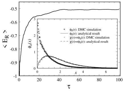
Fig. 4.: DMC description of the hydrogen atom. The time evolution of $E_{R}$ is shown. The inset presents both the radial wave function $\phi_{0}(r)$ and the function $\chi(r)=r\phi_{0}(r)$.

D H${}_{2}^{+}$ Ion

The H${}_{2}^{+}$ ion is held stabilized through a single electron moving in the electric field of two protons separated, at equilibrium, by a distance $R=1.06\AA$[10]. The ground state of this quantum system can not be determined analytically. The numerically determined ground state energy of H${}_{2}^{+}$ is $E_{0}=-16.252\pm 0.002$ eV[10]. The DMC method can be applied in this case as for the hydrogen atom. The Hamiltonian is

$$\hat{H}\;=\;-\,{\hbar^{2}\over 2m}\nabla^{2}\;-\;{e^{2}\over|\mathchoice{{\hbox{\boldmath$\displaystyle r$}}}{{\hbox{\boldmath$\textstyle r$}}}{{\hbox{\boldmath$\scriptstyle r$}}}{{\hbox{\boldmath$\scriptscriptstyle r$}}}\,+\,{1\over 2}\mathchoice{{\hbox{\boldmath$\displaystyle R$}}}{{\hbox{\boldmath$\textstyle R$}}}{{\hbox{\boldmath$\scriptstyle R$}}}{{\hbox{\boldmath$\scriptscriptstyle R$}}}|}\;-\;{e^{2}\over|\mathchoice{{\hbox{\boldmath$\displaystyle r$}}}{{\hbox{\boldmath$\textstyle r$}}}{{\hbox{\boldmath$\scriptstyle r$}}}{{\hbox{\boldmath$\scriptscriptstyle r$}}}\,-\,{1\over 2}\mathchoice{{\hbox{\boldmath$\displaystyle R$}}}{{\hbox{\boldmath$\textstyle R$}}}{{\hbox{\boldmath$\scriptstyle R$}}}{{\hbox{\boldmath$\scriptscriptstyle R$}}}|}$$ (56)

where $\textstyle R$ denotes the separation between the two protons. The results of the DMC description are presented in Fig. 5. The same dimensionless units as in the case of the hydrogen atom were employed and replicas were located initially at the origin, the nuclei being located at $(0,0,\pm R/2)$, for $R=2$. Figure 5 shows that the ground state energy obtained asymptotically is $-16.75$ eV (see Table I) which differs from the more exact numerical value[10] by $0.5$ eV, i.e., by about $3$%. The inset in Fig. 5 shows a plot of the spatial distribution of the replicas, demonstrating that the electronic ground state wave function is nearly spherically symmetric.

E H₂ Molecule

The H₂ molecule is formed by two protons, at equilibrium separated by $R=0.74\AA$[10], and by two electrons. In the Born approximation one considers the proton positions fixed and solves the corresponding stationary Schrödinger equation for the electrons. The wave function of the two electrons must be antisymmetric with respect to exchange of the electrons. In the ground state the electrons are in a singlet spin state

Fig. 5.: DMC description of the H${}_{2}^{+}$ ion. The time evolution of $E_{R}$ is shown. The inset presents the spatial distribution of the replicas, i.e., the electron cloud.

$$\chi(1,2)=\sqrt{1\over 2}\,\left[\chi_{{1\over 2},+{1\over 2}}(1)\chi_{{1\over 2},-{1\over 2}}(2)-\chi_{{1\over 2},-{1\over 2}}(1)\chi_{{1\over 2},+{1\over 2}}(2)\right]$$ (57)

which is antisymmetric. Here $\chi_{\frac{1}{2},\pm\frac{1}{2}}(1,2)$ denotes the wave function of electron $1,2$ in the spin $\frac{1}{2}$ state with magnetic quantum numbers $\pm\frac{1}{2}$. Accordingly, in the wave function of the electronic ground state

$$\Psi_{0}\;=\;\Phi(\mathchoice{{\hbox{\boldmath$\displaystyle r$}}}{{\hbox{\boldmath$\textstyle r$}}}{{\hbox{\boldmath$\scriptstyle r$}}}{{\hbox{\boldmath$\scriptscriptstyle r$}}}_{1},\mathchoice{{\hbox{\boldmath$\displaystyle r$}}}{{\hbox{\boldmath$\textstyle r$}}}{{\hbox{\boldmath$\scriptstyle r$}}}{{\hbox{\boldmath$\scriptscriptstyle r$}}}_{2})\,\chi(1,2)$$ (58)

the factor $\Phi(\mathchoice{{\hbox{\boldmath$\displaystyle r$}}}{{\hbox{\boldmath$\textstyle r$}}}{{\hbox{\boldmath$\scriptstyle r$}}}{{\hbox{\boldmath$\scriptscriptstyle r$}}}_{1},\mathchoice{{\hbox{\boldmath$\displaystyle r$}}}{{\hbox{\boldmath$\textstyle r$}}}{{\hbox{\boldmath$\scriptstyle r$}}}{{\hbox{\boldmath$\scriptscriptstyle r$}}}_{2})$, describing the spatial distribution of the electrons, must be symmetric. This factor can be determined through

$$\Phi(\mathchoice{{\hbox{\boldmath$\displaystyle r$}}}{{\hbox{\boldmath$\textstyle r$}}}{{\hbox{\boldmath$\scriptstyle r$}}}{{\hbox{\boldmath$\scriptscriptstyle r$}}}_{1},\mathchoice{{\hbox{\boldmath$\displaystyle r$}}}{{\hbox{\boldmath$\textstyle r$}}}{{\hbox{\boldmath$\scriptstyle r$}}}{{\hbox{\boldmath$\scriptscriptstyle r$}}}_{2})\;=\;\sqrt{1\over 2}\left(\,\phi(\mathchoice{{\hbox{\boldmath$\displaystyle r$}}}{{\hbox{\boldmath$\textstyle r$}}}{{\hbox{\boldmath$\scriptstyle r$}}}{{\hbox{\boldmath$\scriptscriptstyle r$}}}_{1},\mathchoice{{\hbox{\boldmath$\displaystyle r$}}}{{\hbox{\boldmath$\textstyle r$}}}{{\hbox{\boldmath$\scriptstyle r$}}}{{\hbox{\boldmath$\scriptscriptstyle r$}}}_{2})\;+\;\phi(\mathchoice{{\hbox{\boldmath$\displaystyle r$}}}{{\hbox{\boldmath$\textstyle r$}}}{{\hbox{\boldmath$\scriptstyle r$}}}{{\hbox{\boldmath$\scriptscriptstyle r$}}}_{2},\mathchoice{{\hbox{\boldmath$\displaystyle r$}}}{{\hbox{\boldmath$\textstyle r$}}}{{\hbox{\boldmath$\scriptstyle r$}}}{{\hbox{\boldmath$\scriptscriptstyle r$}}}_{1})\,\right)$$ (59)

where $\phi(\mathchoice{{\hbox{\boldmath$\displaystyle r$}}}{{\hbox{\boldmath$\textstyle r$}}}{{\hbox{\boldmath$\scriptstyle r$}}}{{\hbox{\boldmath$\scriptscriptstyle r$}}}_{1},\mathchoice{{\hbox{\boldmath$\displaystyle r$}}}{{\hbox{\boldmath$\textstyle r$}}}{{\hbox{\boldmath$\scriptstyle r$}}}{{\hbox{\boldmath$\scriptscriptstyle r$}}}_{2})$ is a solution of

$$\left[\,-{\hbar^{2}\over 2m}\left(\nabla_{1}^{2}\,+\,\nabla_{2}^{2}\right)\;-{e^{2}\over|\mathchoice{{\hbox{\boldmath$\displaystyle r$}}}{{\hbox{\boldmath$\textstyle r$}}}{{\hbox{\boldmath$\scriptstyle r$}}}{{\hbox{\boldmath$\scriptscriptstyle r$}}}_{1}-{1\over 2}\mathchoice{{\hbox{\boldmath$\displaystyle R$}}}{{\hbox{\boldmath$\textstyle R$}}}{{\hbox{\boldmath$\scriptstyle R$}}}{{\hbox{\boldmath$\scriptscriptstyle R$}}}|}\;-\;{e^{2}\over|\mathchoice{{\hbox{\boldmath$\displaystyle r$}}}{{\hbox{\boldmath$\textstyle r$}}}{{\hbox{\boldmath$\scriptstyle r$}}}{{\hbox{\boldmath$\scriptscriptstyle r$}}}_{1}+{1\over 2}\mathchoice{{\hbox{\boldmath$\displaystyle R$}}}{{\hbox{\boldmath$\textstyle R$}}}{{\hbox{\boldmath$\scriptstyle R$}}}{{\hbox{\boldmath$\scriptscriptstyle R$}}}|}\;\right.$$ (60)

$$\left.\qquad-\;{e^{2}\over|\mathchoice{{\hbox{\boldmath$\displaystyle r$}}}{{\hbox{\boldmath$\textstyle r$}}}{{\hbox{\boldmath$\scriptstyle r$}}}{{\hbox{\boldmath$\scriptscriptstyle r$}}}_{2}-{1\over 2}\mathchoice{{\hbox{\boldmath$\displaystyle R$}}}{{\hbox{\boldmath$\textstyle R$}}}{{\hbox{\boldmath$\scriptstyle R$}}}{{\hbox{\boldmath$\scriptscriptstyle R$}}}|}\;-\;{e^{2}\over|\mathchoice{{\hbox{\boldmath$\displaystyle r$}}}{{\hbox{\boldmath$\textstyle r$}}}{{\hbox{\boldmath$\scriptstyle r$}}}{{\hbox{\boldmath$\scriptscriptstyle r$}}}_{2}+{1\over 2}\mathchoice{{\hbox{\boldmath$\displaystyle R$}}}{{\hbox{\boldmath$\textstyle R$}}}{{\hbox{\boldmath$\scriptstyle R$}}}{{\hbox{\boldmath$\scriptscriptstyle R$}}}|}\;+\;{e^{2}\over|\mathchoice{{\hbox{\boldmath$\displaystyle r$}}}{{\hbox{\boldmath$\textstyle r$}}}{{\hbox{\boldmath$\scriptstyle r$}}}{{\hbox{\boldmath$\scriptscriptstyle r$}}}_{1}-\mathchoice{{\hbox{\boldmath$\displaystyle r$}}}{{\hbox{\boldmath$\textstyle r$}}}{{\hbox{\boldmath$\scriptstyle r$}}}{{\hbox{\boldmath$\scriptscriptstyle r$}}}_{2}|}\,\right]\,\phi(\mathchoice{{\hbox{\boldmath$\displaystyle r$}}}{{\hbox{\boldmath$\textstyle r$}}}{{\hbox{\boldmath$\scriptstyle r$}}}{{\hbox{\boldmath$\scriptscriptstyle r$}}}_{1},\mathchoice{{\hbox{\boldmath$\displaystyle r$}}}{{\hbox{\boldmath$\textstyle r$}}}{{\hbox{\boldmath$\scriptstyle r$}}}{{\hbox{\boldmath$\scriptscriptstyle r$}}}_{2})\;$$ (61)

$$\qquad\qquad\qquad\qquad\qquad\qquad\qquad=\;E_{0}\,\phi(\mathchoice{{\hbox{\boldmath$\displaystyle r$}}}{{\hbox{\boldmath$\textstyle r$}}}{{\hbox{\boldmath$\scriptstyle r$}}}{{\hbox{\boldmath$\scriptscriptstyle r$}}}_{1},\mathchoice{{\hbox{\boldmath$\displaystyle r$}}}{{\hbox{\boldmath$\textstyle r$}}}{{\hbox{\boldmath$\scriptstyle r$}}}{{\hbox{\boldmath$\scriptscriptstyle r$}}}_{2})$$ (62)

TABLE I.: Results obtained during two different simulations performed on four quantum systems listed in the first column. During Simulation I (II) the initial number of replicas was 500 (4000), the time step $\Delta\tau=0.1$ (0.05), the length of simulation $\tau=1000\Delta\tau$ ($2000\Delta\tau$), the random number generator seed 1 and the number of boxes used to calculate the spatial distribution of the replicas 200 (400). $\langle E_{R}\rangle$ and $\delta E_{R}$ are defined in the text. $\Delta t$ represents the actual running time of the simulation on a HP-9000 (series 700) workstation. For the hydrogen atom the energies are given both in dimensionless units and in eV (in parenthesis), respectively. For comparison, $E_{0}$ in the last column represents the exact value (analytical or obtained through an alternative numerical method) of the corresponding ground state energy.

	Simulation I			Simulation II
Quantum system	$\langle E_{R}\rangle$	$\delta E_{R}$	$\Delta t$	$\langle E_{R}\rangle$	$\delta E_{R}$	$\Delta t$	$E_{0}$
Harmonic oscillator	0.505	0.094	8 sec	0.500	0.048	4 min	0.5
Morse oscillator	-0.1236	0.0749	10 sec	-0.1245	0.0330	4 min	-0.125
Hydrogen atom	-0.495	0.080	18 sec	-0.505	0.040	5 min	0.5
	(-13.477 eV)	(2.186 eV)		(-13.752 eV)	(1.093 eV)		(13.6 eV)
H${}_{2}^{+}$ ion	-16.753 eV	2.869 eV	40 sec	-16.476 eV	1.389 eV	11 min	-16.25(2) eVa
H2 molecule	-30.973 eV	3.638 eV	55 sec	-31.968 eV	1.754 eV	16 min	-31.6(87) eVa

^a Numerical values calculated based upon the heat of dissociation given by Hertzberg[10].

The Schrödinger equation (62) cannot be solved analytically. The available numerical result for the ground state energy of H₂ is $E_{0}=-31.688\pm 0.013$ eV[10]. The results of the diffusion Monte Carlo simulation for H₂ are shown in Fig. 6. The same dimensionless units as in the case of the hydrogen atom were employed and the replicas at $\tau=0$ were located initially at $\{(0,0,1)(0,0,-1)\}$; the position of the protons were $(0,0,\pm R/2)$, with $R=1.398$. The simulation took about $55$ seconds to complete and the obtained ground state energy was $E_{0}=-30.973$ eV (see Table I). This result differs from the exact energy by $0.715$ eV, i.e., by $2.3$%. The inset of Fig. 6 shows the spatial distribution of the replicas which is nearly spherically symmetric. In Fig. 7 we present the results of a calculation in which an unphysically large $R$ value of $8.398$ was assumed. In this case the distribution of the electronic cloud around the protons is clearly anisotropic, the energy of the electrons is still negative.

Fig. 6.: DMC description of the electronic ground state of the H₂ molecule. The time evolution of $E_{R}$ is shown. The inset presents the spatial distribution of the replicas, i.e., the electron cloud.

Fig. 7.: $E_{R}$ vs. $\tau$ and the spatial distribution of the replicas (inset) at the end of the simulation for the H₂ molecule for an unphysically large separation between the two protons of 8.398 Bohr radius.

V Discussion

In this article, we have presented a detailed account of the path integral formulation of the DMC method devised for calculating simultaneously the ground state energy and wave function of an arbitrary quantum system. A simple numerical algorithm based on the DMC method has been formulated and a computer program, based on this algorithm, has been applied to determine numerically the ground state of a few quantum systems of pedagogical interest.

The DMC algorithm, as presented in this article, is quite unstable numerically. We want to demonstrate here the need for an improvement of the method. This need arises due to the strong fluctuations stemming from the birth-death processes employed in this method. These fluctuations affect the reference energy $E_{R}(\tau)$ which is expected to converge to the ground state energy. This convergence is observed only for the value of $\langle E_{R}\rangle$ defined through equation (50). The actual time dependence of $E_{R}$ is presented in Fig. 8 for the case of the harmonic oscillator. The fluctuations in $E_{R}$ are large, but symmetrically distributed around $\langle E_{R}\rangle$ which explains the good agreement between the result of the simulation with the exact result. Attempts to use our DMC program to calculate the electronic ground state energy of the H${}_{2}^{+}$ ion and H₂ molecule as a function of the separation between the two protons, which would allow one to determine the equilibrium separation from the minimum of this dependence, have failed due to large fluctuations in $E_{R}$.

The DMC algorithm can be significantly improved resorting to a method called “importance sampling”[1, 9]. The basic idea of this method is to change the probability distribution of the replicas in a controlled way. This can be achieved by reformulating (10) such that the resulting equation has a solution $\Psi(x,\tau)$ multiplied by an approximation of the ground state wave function, the latter being obtained, for example, from a variational method. Application of the DMC method to this new equation yields then replicas which spend more time in “important” regions of the configuration space where the wave function $\Psi(x,\tau)$ is expected to be large. For details regarding importance sampling the reader is referred to the literature cited[1, 2, 9].

Any implementation of the DMC method leads to systematic errors due to the use of a finite time step $\Delta\tau$. Apparently these errors can be reduced to zero by choosing $\Delta\tau\rightarrow 0$. Unfortunately, this is not the case. Even worse: making the time step shorter and shorter does not only increase the needed computer time, but also renders the successive generations of replicas more and more correlated such that their distribution actually departs more and more from the ground state wave function. For each quantum system investigated it is necessary to find the most convenient value of $\Delta\tau$ which is short enough to produce small systematic errors and at the same time is long enough to keep the successive distributions of replicas sufficiently uncorrelated.

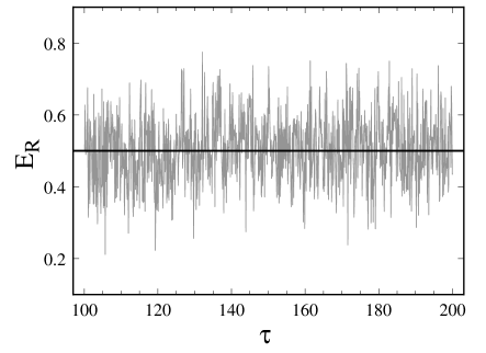
Fig. 8.: Fluctuations of $E_{R}$ about its average value $\langle E_{R}\rangle\approx 0.5$ well after the distribution of replicas reached its stationary form. The relatively large fluctuations are due to the birth–death processes which persist even if the replicas are distributed according to the exact ground state wave function $\phi_{0}(x)$ and the reference energy $E_{R}$ has been adapted to the exact ground state energy.

In order to apply the DMC method to calculate the ground state properties of a system with interacting fermions one has to treat, as mentioned above, the “sign problem” due to the antisymmetry property of the many-fermion wave function. Two principle methods, the fixed–node method[13, 1] and the release–node method[14, 1], have been proposed to deal with this problem.

Once some kind of importance sampling is implemented and the sign–problem, in the case of many–fermion systems, is resolved, the DMC method can be used to compute ground state properties for molecules or molecular clusters[9] and for quantum spin, boson and fermion systems[15]. The method is also applicable to the study of ground–state phase transitions due to quantum fluctuations, a topic of modern condensed matter physics[15].

Finally we would like to mention that the DMC method has been extended and successfully applied to the study of the excited states of molecules and clusters[9] and also to the study of finite temperature properties of different condensed matter systems. Also, the DMC method has been successfully applied in quantum field theories[16].

VI Acknowledgments

This work has been supported by a National Science Foundation REU fellowship to B.F., by funds of the University of Illinois at Urbana-Champaign, and by a grant from the National Science Foundation (BIR-9318159).

REFERENCES

- [1] D. Ceperley and B. Alder, “Quantum Monte Carlo”, Science 231, 555–560 (1986).
- [2] M. H. Kalos and P. A. Whitlock, Monte Carlo methods (J. Wiley & Sons, New York, 1986).
- [3] J. B. Anderson, “A random–walk simulation of the Schrödinger equation: H”, J. Chem. Phys. 63, 1499–1503 (1975).
- [4] W. H. Press, S. A. Teukolsky, W. T. Vetterling and B. P. Flannery, Numerical recipes in C : the art of scientific computing (Cambridge University Press, Cambridge, 1992), 2nd edn.
- [5] L. D. Landau and E. M. Lifshitz, Quantum Mechanics, vol. 3 of Course of Theoretical Physics (Pergamon Press, Oxford, 1977).
- [6] R. P. Feynman and A. R. Hibbs, Quantum mechanics and path integrals (McGraw-Hill, New York, 1965).
- [7] D. Khandekar, S. Lawande and K. B. Hagwat, Path Integral Methods and Their Applications (World Scientific, London, 1993).
- [8] S. E. Koonin, Computational Physics (Benjamin, Reading, MA, 1986).
- [9] M. A. Suhm and R. O. Watts, “Quantum Monte Carlo studies of vibrational states in molecules and clusters”, Phys. Rep. 204, 293–329 (1991).
- [10] G. Herzberg, Molecular Spectra and Molecular Structure (Van Nostrand, New York 1950).
- [11] The program was written is the C programming language. A copy of the source code is freely available from one of the authors (K.S.).
- [12] L. Infeld and T. E. Hull, “The factorization method”, Rev. Mod. Phys. 23, 21–68 (1951).
- [13] P. J. Reynolds, D. M. Ceperley, B. J. Adler and J. W. A. Lester, “Fixed–node quantum Monte Carlo for molecules”, J. Chem. Phys. 77, 5593–5603 (1982).
- [14] D. M. Ceperley and B. J. Adler, “Quantum Monte Carlo for molecules: Green’s function and nodal release”, J. Chem. Phys. 81, 5833–5844 (1984).
- [15] M. Suzuki, Quantum Monte Carlo methods in condensed matter physics (World Scientific, Singapore, 1993).
- [16] T. Barnes and G. J. Daniell, “Numerical Solution of Field Theories Using Random Walks”, Nucl. Phys. B257, 173–198 (1985).