Boundary Integral Method for Stationary States of Two-Dimensional Quantum Systems

Abstract

The boundary integral method for calculating the stationary states of a quantum particle in nano-devices and quantum billiards is presented in detail at an elementary level. According to the method, wave functions inside the domain of the device or billiard are expressed in terms of line integrals of the wave function and its normal derivative along the domain’s boundary; the respective energy eigenvalues are obtained as the roots of Fredholm determinants. Numerical implementations of the method are described and applied to determine the energy level statistics of billiards with circular and stadium shapes and demonstrate the quantum mechanical characteristics of chaotic motion. The treatment of other examples as well as the advantages and limitations of the boundary integral method are discussed.

I Introduction

Recent advances in nanotechnology, based on advanced crystal growth and lithographic techniques, have opened an avenue to fabricate very small and clean electronic devices, known as nano-devices[1]. The charge carriers (electrons) in such devices, through gate voltages, are confined to one or two spatial dimensions. At very low temperatures, the spatial extent of the systems along the direction of confinement is comparable to the Fermi wavelength of the electrons. Quantum dots and quantum wires are examples of quasi zero- and one-dimensional nano-devices in which confinement of the electrons occur along all three and along two spatial directions, respectively, while in the inversion layer of narrow-gap semiconductor heterostructures the electrons are confined along the direction perpendicular to the layer. Quantum dots are relevant in the study of the Coulomb blockade phenomena[2], while quantum wires are experimental realizations of so-called Luttinger liquids[3].

The motion of the electrons in a clean two-dimensional nano-device is ballistic, i.e., the electrons are scattered mainly by the device boundaries and not by impurities. The device boundaries, due to high precision lithography, may have arbitrary shapes and are very sharp, i.e., the electrical potential changes abruptly on atomic scales. As a result, the behavior of such two-dimensional nano-devices, which exhibit quantum confinement in one direction and free motion of the electrons in a finite two-dimensional domain of sub-micron size, is governed by single-electron (particle) physics, and can be described theoretically by solving the corresponding Schrödinger wave equation. Such nano-devices can be considered as quantum mechanical analogue of classical billiard systems[4] in which point like particles bounce inside a two-dimensional (2D) region ${\cal D}$ delimited by the contour $\Gamma$. An idealized quantum billiard confines a quantum particle inside a 2D infinite potential well; the shape of the infinite well being determined by $\Gamma$.

Quantum billiards represent models of nano-devices which play an important role in modern semiconductor industry[1]. The experimental study, via STM techniques, of quantum billiards provides a new testing-ground for the predictions of quantum mechanics[1]. The study of quantum billiards allows one to investigate also the quantum signatures of classical chaos. It is known that non-integrable classical systems are chaotic, i.e., the phase space trajectory of the system exhibits exponential sensitivity to the initial conditions. In the case of billiards, the chaotic behavior is caused by the irregularities of the boundary and not by the complexity of the interaction in the system (e.g., scattering of the particle from randomly distributed impurities). Since the concept of “phase space trajectory” loses its meaning in quantum mechanics, one can naturally ask oneself what is the quantum mechanical analogue of (classical) chaos, or more precisely, is there any detectable difference between the behavior of a quantum system with chaotic- and non-chaotic classical limit, respectively.

The answer to these questions should be sought in the characteristics of the fluctuations of the energy levels of the quantum billiard systems[5, 6]. Thus, in order to study the physical properties of quantum billiards one needs to find first the corresponding energy spectrum by solving the time independent Schrödinger equation

$$\hat{H}\psi_{n}(\mathchoice{{\hbox{\boldmath$\displaystyle r$}}}{{\hbox{\boldmath$\textstyle r$}}}{{\hbox{\boldmath$\scriptstyle r$}}}{{\hbox{\boldmath$\scriptscriptstyle r$}}})\;\equiv\;\left[-\frac{\hbar^{2}}{2m}\nabla^{2}+V(\mathchoice{{\hbox{\boldmath$\displaystyle r$}}}{{\hbox{\boldmath$\textstyle r$}}}{{\hbox{\boldmath$\scriptstyle r$}}}{{\hbox{\boldmath$\scriptscriptstyle r$}}})\right]\psi_{n}(\mathchoice{{\hbox{\boldmath$\displaystyle r$}}}{{\hbox{\boldmath$\textstyle r$}}}{{\hbox{\boldmath$\scriptstyle r$}}}{{\hbox{\boldmath$\scriptscriptstyle r$}}})\;=\;E_{n}\psi_{n}(\mathchoice{{\hbox{\boldmath$\displaystyle r$}}}{{\hbox{\boldmath$\textstyle r$}}}{{\hbox{\boldmath$\scriptstyle r$}}}{{\hbox{\boldmath$\scriptscriptstyle r$}}})\;,$$ (1)

where $\hat{H}$ is the Hamiltonian of the system, $V(\mathchoice{{\hbox{\boldmath$\displaystyle r$}}}{{\hbox{\boldmath$\textstyle r$}}}{{\hbox{\boldmath$\scriptstyle r$}}}{{\hbox{\boldmath$\scriptscriptstyle r$}}})$ is the potential energy, and $\psi_{n}$ is the eigenfunction corresponding to the energy eigenvalue $E_{n}$. In general, in (1) the potential $V(\mathchoice{{\hbox{\boldmath$\displaystyle r$}}}{{\hbox{\boldmath$\textstyle r$}}}{{\hbox{\boldmath$\scriptstyle r$}}}{{\hbox{\boldmath$\scriptscriptstyle r$}}})$ does not contain the term corresponding to the infinite potential well; the effect of the later is reflected by the “hard-wall” (i.e., Dirichlet) boundary conditions at the billiard boundary. The spectrum is discrete and the distribution of the energy levels $E_{n}$ is determined by the form of the potential and by the boundary conditions.

Eq.(1) can be solved analytically only for very few special cases, when the system is integrable, i.e., when there exists, besides the energy, a second conserved physical quantity. Such examples, like a quantum particle in a rectangular or circular infinite potential well, are discussed in most of the quantum mechanics textbooks[7] and in some recent publications[8], as well. However, for a generic quantum billiard the energy spectrum can be determined only numerically, and the description of such numerical methods lacks in all widely used quantum mechanics textbooks.

The purpose of the present article is to fill this gap by providing the reader with a self-contained and practical introduction to a powerful numerical method, known as the Boundary Integral Method (BIM), for calculating the energy levels of a 2D quantum system, e.g., a quantum billiard. While the BIM, sometimes also referred to as the Boundary Element Method (BEM), has been extensively used for many years for solving different engineering problems[9, 10, 11], its application for calculating energy spectra of quantum billiards has emerged only recently[12, 13, 14, 15, 16].

Before we embark on our presentation of the BIM for calculating energy spectra of 2D quantum systems, let us first mention a few other frequently used numerical methods in the same context.

Essentially all numerical methods devised to solve the single particle Schrödinger equation (1) can be classified in two groups. The methods belonging to the first group assume that one readily knows a complete set of orthonormal functions $\left\{\phi_{m}(\mathchoice{{\hbox{\boldmath$\displaystyle r$}}}{{\hbox{\boldmath$\textstyle r$}}}{{\hbox{\boldmath$\scriptstyle r$}}}{{\hbox{\boldmath$\scriptscriptstyle r$}}})\right\}$ which obey the desired boundary conditions along the billiard boundary. By expanding the unknown energy eigenfunctions

$$\psi_{n}(\mathchoice{{\hbox{\boldmath$\displaystyle r$}}}{{\hbox{\boldmath$\textstyle r$}}}{{\hbox{\boldmath$\scriptstyle r$}}}{{\hbox{\boldmath$\scriptscriptstyle r$}}})\;=\;\sum_{m}c_{nm}\phi_{m}(\mathchoice{{\hbox{\boldmath$\displaystyle r$}}}{{\hbox{\boldmath$\textstyle r$}}}{{\hbox{\boldmath$\scriptstyle r$}}}{{\hbox{\boldmath$\scriptscriptstyle r$}}})\;,$$ (2)

the Schrödinger equation is converted into the familiar system of homogeneous linear equations for the coefficients $c_{nm}$

$$\sum_{m}\left(H_{nm}-E_{n}\delta_{nm}\right)c_{nm}\;=\;0\;,$$ (3)

Here $\delta_{nm}$ is the Kronecker-delta (equal to $1$ for $n=m$ and zero otherwise), and the matrix elements of the Hamiltonian are

$$H_{nm}\;=\;\int\!\!d\mathchoice{{\hbox{\boldmath$\displaystyle r$}}}{{\hbox{\boldmath$\textstyle r$}}}{{\hbox{\boldmath$\scriptstyle r$}}}{{\hbox{\boldmath$\scriptscriptstyle r$}}}\;\phi_{n}^{*}(\mathchoice{{\hbox{\boldmath$\displaystyle r$}}}{{\hbox{\boldmath$\textstyle r$}}}{{\hbox{\boldmath$\scriptstyle r$}}}{{\hbox{\boldmath$\scriptscriptstyle r$}}})\hat{H}\;\phi_{m}(\mathchoice{{\hbox{\boldmath$\displaystyle r$}}}{{\hbox{\boldmath$\textstyle r$}}}{{\hbox{\boldmath$\scriptstyle r$}}}{{\hbox{\boldmath$\scriptscriptstyle r$}}})\;.$$ (4)

Equation (3) admits non-trivial solutions (energy eigenstates or stationary states) only for those values of $E_{n}$ (the energy eigenvalues) which satisfy the condition

$$\text{det}\left|H_{nm}-E_{n}\delta_{nm}\right|\;=\;0\;.$$ (5)

This condition can be employed to determine the $E_{n}$’s.

When the billiard boundary is irregular, in general, it is impossible to find analytical expressions for the functions $\phi_{m}(\mathchoice{{\hbox{\boldmath$\displaystyle r$}}}{{\hbox{\boldmath$\textstyle r$}}}{{\hbox{\boldmath$\scriptstyle r$}}}{{\hbox{\boldmath$\scriptscriptstyle r$}}})$ and, therefore, the method as described fails. However, in this case one can overcome the previously mentioned difficulty by either performing a coordinate transformation which renders the boundary highly regular, or by extending the system, fitting the billiard inside a rectangle or circle along which the Dirichlet boundary conditions apply. Now a complete set of orthonormal functions can be easily found, but the price one pays in both cases is that the corresponding Hamiltonian becomes more complicated: in the former case the simple form of the kinetic energy is altered[18] while in the latter case the potential energy is modified[19], i.e., $V(\mathchoice{{\hbox{\boldmath$\displaystyle r$}}}{{\hbox{\boldmath$\textstyle r$}}}{{\hbox{\boldmath$\scriptstyle r$}}}{{\hbox{\boldmath$\scriptscriptstyle r$}}})=0$ inside ${\cal D}$ and $V(\mathchoice{{\hbox{\boldmath$\displaystyle r$}}}{{\hbox{\boldmath$\textstyle r$}}}{{\hbox{\boldmath$\scriptstyle r$}}}{{\hbox{\boldmath$\scriptscriptstyle r$}}})=\infty$ (in practice a suitably chosen large value) outside ${\cal D}$.

The second class of numerical methods intended to calculate billiard spectra regard Eq.(1) as a partial differential equation for which the general solution is formally given by (2) for some conveniently chosen basis functions $\phi_{m}(\mathchoice{{\hbox{\boldmath$\displaystyle r$}}}{{\hbox{\boldmath$\textstyle r$}}}{{\hbox{\boldmath$\scriptstyle r$}}}{{\hbox{\boldmath$\scriptscriptstyle r$}}})$. The energy eigenfunctions and eigenvalues are determined by requiring the general solution (2) to obey the Dirichlet boundary conditions along $\partial{\cal D}$. Of course, the boundary conditions can be met only for particular values of the energy, i.e., the energy eigenvalues. Heller[20] used this method choosing as the basis functions plane waves, while a more general and systematic implementation of this method in plane polar coordinates is described by Schmit[21].

The BIM is an efficient alternative to the above mentioned two classes of methods for solving numerically the Schrödinger equation. We shall consider its application only for two-dimensional systems. The BIM will allow us to study the quantum analogue of classical chaotic systems and reveal that chaotic behavior is reflected in the spacing of the energy eigenvalues $E_{n}$. For this purpose, the BIM is formulated in Sec. II and is applied, in Sec. III, to the spectra of circular, stadium and generalized stadium billiards. In Sec. IV we discuss further examples to which the BIM can be applied. In Sec. V we present concluding remarks.

II The Boundary Integral Method

Consider a quantum particle of mass $m$ moving in a finite, simply connected region ${\cal D}$, experiencing the potential $V(\mathchoice{{\hbox{\boldmath$\displaystyle r$}}}{{\hbox{\boldmath$\textstyle r$}}}{{\hbox{\boldmath$\scriptstyle r$}}}{{\hbox{\boldmath$\scriptscriptstyle r$}}})$ and being governed by the Hamiltonian

$$\hat{H}\;=\;-\frac{\hbar^{2}}{2m}\nabla^{2}+V(\mathchoice{{\hbox{\boldmath$\displaystyle r$}}}{{\hbox{\boldmath$\textstyle r$}}}{{\hbox{\boldmath$\scriptstyle r$}}}{{\hbox{\boldmath$\scriptscriptstyle r$}}})\;.$$ (6)

The energy spectrum of the particle can be determined from the time-independent Schrödinger equation (1) together with the boundary conditions for the wave functions $\psi_{n}(\mathchoice{{\hbox{\boldmath$\displaystyle r$}}}{{\hbox{\boldmath$\textstyle r$}}}{{\hbox{\boldmath$\scriptstyle r$}}}{{\hbox{\boldmath$\scriptscriptstyle r$}}})$ specified on a closed curve $\Gamma=\partial{\cal D}$ which delimits the region ${\cal D}$.

The Schrödinger equation (1) is an implicit equation for $E_{n}$ and $\psi_{n}(\mathchoice{{\hbox{\boldmath$\displaystyle r$}}}{{\hbox{\boldmath$\textstyle r$}}}{{\hbox{\boldmath$\scriptstyle r$}}}{{\hbox{\boldmath$\scriptscriptstyle r$}}})$. This differential equation can be replaced by an implicit integral equation which can also serve to determine $E_{n}$ and $\psi_{n}(\mathchoice{{\hbox{\boldmath$\displaystyle r$}}}{{\hbox{\boldmath$\textstyle r$}}}{{\hbox{\boldmath$\scriptstyle r$}}}{{\hbox{\boldmath$\scriptscriptstyle r$}}})$. For this purpose, one introduces the Green’s function, $G(\mathchoice{{\hbox{\boldmath$\displaystyle r$}}}{{\hbox{\boldmath$\textstyle r$}}}{{\hbox{\boldmath$\scriptstyle r$}}}{{\hbox{\boldmath$\scriptscriptstyle r$}}},\mathchoice{{\hbox{\boldmath$\displaystyle r^{\prime}$}}}{{\hbox{\boldmath$\textstyle r^{\prime}$}}}{{\hbox{\boldmath$\scriptstyle r^{\prime}$}}}{{\hbox{\boldmath$\scriptscriptstyle r^{\prime}$}}};E)$ of the operator $E-\hat{H}$, defined as the solution of

$$[E-\hat{H}(\mathchoice{{\hbox{\boldmath$\displaystyle r$}}}{{\hbox{\boldmath$\textstyle r$}}}{{\hbox{\boldmath$\scriptstyle r$}}}{{\hbox{\boldmath$\scriptscriptstyle r$}}})]\,G(\mathchoice{{\hbox{\boldmath$\displaystyle r$}}}{{\hbox{\boldmath$\textstyle r$}}}{{\hbox{\boldmath$\scriptstyle r$}}}{{\hbox{\boldmath$\scriptscriptstyle r$}}},\mathchoice{{\hbox{\boldmath$\displaystyle r^{\prime}$}}}{{\hbox{\boldmath$\textstyle r^{\prime}$}}}{{\hbox{\boldmath$\scriptstyle r^{\prime}$}}}{{\hbox{\boldmath$\scriptscriptstyle r^{\prime}$}}};E)\;=\;\delta(\mathchoice{{\hbox{\boldmath$\displaystyle r$}}}{{\hbox{\boldmath$\textstyle r$}}}{{\hbox{\boldmath$\scriptstyle r$}}}{{\hbox{\boldmath$\scriptscriptstyle r$}}}-\mathchoice{{\hbox{\boldmath$\displaystyle r^{\prime}$}}}{{\hbox{\boldmath$\textstyle r^{\prime}$}}}{{\hbox{\boldmath$\scriptstyle r^{\prime}$}}}{{\hbox{\boldmath$\scriptscriptstyle r^{\prime}$}}})\;,$$ (7)

where $\delta(\mathchoice{{\hbox{\boldmath$\displaystyle r$}}}{{\hbox{\boldmath$\textstyle r$}}}{{\hbox{\boldmath$\scriptstyle r$}}}{{\hbox{\boldmath$\scriptscriptstyle r$}}}-\mathchoice{{\hbox{\boldmath$\displaystyle r^{\prime}$}}}{{\hbox{\boldmath$\textstyle r^{\prime}$}}}{{\hbox{\boldmath$\scriptstyle r^{\prime}$}}}{{\hbox{\boldmath$\scriptscriptstyle r^{\prime}$}}})$ is the two-dimensional $\delta$-function, $E$ is a complex variable , and $\textstyle r$, $\textstyle r^{\prime}$ are arbitrary points in ${\cal D}$. Multiplying Eq.(1) by $G(\mathchoice{{\hbox{\boldmath$\displaystyle r$}}}{{\hbox{\boldmath$\textstyle r$}}}{{\hbox{\boldmath$\scriptstyle r$}}}{{\hbox{\boldmath$\scriptscriptstyle r$}}},\mathchoice{{\hbox{\boldmath$\displaystyle r^{\prime}$}}}{{\hbox{\boldmath$\textstyle r^{\prime}$}}}{{\hbox{\boldmath$\scriptstyle r^{\prime}$}}}{{\hbox{\boldmath$\scriptscriptstyle r^{\prime}$}}};E)$, Eq.(7) by $\psi_{n}(\mathchoice{{\hbox{\boldmath$\displaystyle r$}}}{{\hbox{\boldmath$\textstyle r$}}}{{\hbox{\boldmath$\scriptstyle r$}}}{{\hbox{\boldmath$\scriptscriptstyle r$}}})$, and adding the resulting equations yield

$$\psi_{n}(\mathchoice{{\hbox{\boldmath$\displaystyle r$}}}{{\hbox{\boldmath$\textstyle r$}}}{{\hbox{\boldmath$\scriptstyle r$}}}{{\hbox{\boldmath$\scriptscriptstyle r$}}})\delta(\mathchoice{{\hbox{\boldmath$\displaystyle r$}}}{{\hbox{\boldmath$\textstyle r$}}}{{\hbox{\boldmath$\scriptstyle r$}}}{{\hbox{\boldmath$\scriptscriptstyle r$}}}-\mathchoice{{\hbox{\boldmath$\displaystyle r^{\prime}$}}}{{\hbox{\boldmath$\textstyle r^{\prime}$}}}{{\hbox{\boldmath$\scriptstyle r^{\prime}$}}}{{\hbox{\boldmath$\scriptscriptstyle r^{\prime}$}}})+\left(E_{n}-E\right)\psi_{n}(\mathchoice{{\hbox{\boldmath$\displaystyle r$}}}{{\hbox{\boldmath$\textstyle r$}}}{{\hbox{\boldmath$\scriptstyle r$}}}{{\hbox{\boldmath$\scriptscriptstyle r$}}})G(\mathchoice{{\hbox{\boldmath$\displaystyle r$}}}{{\hbox{\boldmath$\textstyle r$}}}{{\hbox{\boldmath$\scriptstyle r$}}}{{\hbox{\boldmath$\scriptscriptstyle r$}}},\mathchoice{{\hbox{\boldmath$\displaystyle r^{\prime}$}}}{{\hbox{\boldmath$\textstyle r^{\prime}$}}}{{\hbox{\boldmath$\scriptstyle r^{\prime}$}}}{{\hbox{\boldmath$\scriptscriptstyle r^{\prime}$}}};E)\;=\;G(\mathchoice{{\hbox{\boldmath$\displaystyle r$}}}{{\hbox{\boldmath$\textstyle r$}}}{{\hbox{\boldmath$\scriptstyle r$}}}{{\hbox{\boldmath$\scriptscriptstyle r$}}},\mathchoice{{\hbox{\boldmath$\displaystyle r^{\prime}$}}}{{\hbox{\boldmath$\textstyle r^{\prime}$}}}{{\hbox{\boldmath$\scriptstyle r^{\prime}$}}}{{\hbox{\boldmath$\scriptscriptstyle r^{\prime}$}}};E)\hat{H}\psi_{n}(\mathchoice{{\hbox{\boldmath$\displaystyle r$}}}{{\hbox{\boldmath$\textstyle r$}}}{{\hbox{\boldmath$\scriptstyle r$}}}{{\hbox{\boldmath$\scriptscriptstyle r$}}})-\psi_{n}(\mathchoice{{\hbox{\boldmath$\displaystyle r$}}}{{\hbox{\boldmath$\textstyle r$}}}{{\hbox{\boldmath$\scriptstyle r$}}}{{\hbox{\boldmath$\scriptscriptstyle r$}}})\hat{H}G(\mathchoice{{\hbox{\boldmath$\displaystyle r$}}}{{\hbox{\boldmath$\textstyle r$}}}{{\hbox{\boldmath$\scriptstyle r$}}}{{\hbox{\boldmath$\scriptscriptstyle r$}}},\mathchoice{{\hbox{\boldmath$\displaystyle r^{\prime}$}}}{{\hbox{\boldmath$\textstyle r^{\prime}$}}}{{\hbox{\boldmath$\scriptstyle r^{\prime}$}}}{{\hbox{\boldmath$\scriptscriptstyle r^{\prime}$}}};E)\;.$$ (8)

We consider now Eq.(8) for $E=E_{n}$. In this case the second term on the LHS vanishes, provided that $G$ is finite (i.e., has no poles) at $E_{n}$. A necessary (but not sufficient) condition is that $G$ does not obey the same boundary conditions as $\psi_{n}$. Inserting the Hamiltonian (6) in the RHS of Eq.(8) eliminates the terms containing the potential energy $V(\mathchoice{{\hbox{\boldmath$\displaystyle r$}}}{{\hbox{\boldmath$\textstyle r$}}}{{\hbox{\boldmath$\scriptstyle r$}}}{{\hbox{\boldmath$\scriptscriptstyle r$}}})$ and Eq.(8) becomes

$$\psi_{n}(\mathchoice{{\hbox{\boldmath$\displaystyle r$}}}{{\hbox{\boldmath$\textstyle r$}}}{{\hbox{\boldmath$\scriptstyle r$}}}{{\hbox{\boldmath$\scriptscriptstyle r$}}})\delta(\mathchoice{{\hbox{\boldmath$\displaystyle r$}}}{{\hbox{\boldmath$\textstyle r$}}}{{\hbox{\boldmath$\scriptstyle r$}}}{{\hbox{\boldmath$\scriptscriptstyle r$}}}-\mathchoice{{\hbox{\boldmath$\displaystyle r^{\prime}$}}}{{\hbox{\boldmath$\textstyle r^{\prime}$}}}{{\hbox{\boldmath$\scriptstyle r^{\prime}$}}}{{\hbox{\boldmath$\scriptscriptstyle r^{\prime}$}}})\;=\;\frac{\hbar^{2}}{2m}\left[\psi_{n}(\mathchoice{{\hbox{\boldmath$\displaystyle r$}}}{{\hbox{\boldmath$\textstyle r$}}}{{\hbox{\boldmath$\scriptstyle r$}}}{{\hbox{\boldmath$\scriptscriptstyle r$}}})\nabla^{2}G\left(\mathchoice{{\hbox{\boldmath$\displaystyle r$}}}{{\hbox{\boldmath$\textstyle r$}}}{{\hbox{\boldmath$\scriptstyle r$}}}{{\hbox{\boldmath$\scriptscriptstyle r$}}},\mathchoice{{\hbox{\boldmath$\displaystyle r^{\prime}$}}}{{\hbox{\boldmath$\textstyle r^{\prime}$}}}{{\hbox{\boldmath$\scriptstyle r^{\prime}$}}}{{\hbox{\boldmath$\scriptscriptstyle r^{\prime}$}}};E_{n}\right)-G\left(\mathchoice{{\hbox{\boldmath$\displaystyle r$}}}{{\hbox{\boldmath$\textstyle r$}}}{{\hbox{\boldmath$\scriptstyle r$}}}{{\hbox{\boldmath$\scriptscriptstyle r$}}},\mathchoice{{\hbox{\boldmath$\displaystyle r^{\prime}$}}}{{\hbox{\boldmath$\textstyle r^{\prime}$}}}{{\hbox{\boldmath$\scriptstyle r^{\prime}$}}}{{\hbox{\boldmath$\scriptscriptstyle r^{\prime}$}}};E_{n}\right)\nabla^{2}\psi_{n}(\mathchoice{{\hbox{\boldmath$\displaystyle r$}}}{{\hbox{\boldmath$\textstyle r$}}}{{\hbox{\boldmath$\scriptstyle r$}}}{{\hbox{\boldmath$\scriptscriptstyle r$}}})\right]\;.$$ (9)

Recalling the identity $u\nabla^{2}v=\nabla(u\nabla v)-\nabla u\nabla v$, valid for any differentiable functions $u(\mathchoice{{\hbox{\boldmath$\displaystyle r$}}}{{\hbox{\boldmath$\textstyle r$}}}{{\hbox{\boldmath$\scriptstyle r$}}}{{\hbox{\boldmath$\scriptscriptstyle r$}}})$ and $v(\mathchoice{{\hbox{\boldmath$\displaystyle r$}}}{{\hbox{\boldmath$\textstyle r$}}}{{\hbox{\boldmath$\scriptstyle r$}}}{{\hbox{\boldmath$\scriptscriptstyle r$}}})$, the RHS of the above equation can be written as a divergence

$$\psi_{n}(\mathchoice{{\hbox{\boldmath$\displaystyle r$}}}{{\hbox{\boldmath$\textstyle r$}}}{{\hbox{\boldmath$\scriptstyle r$}}}{{\hbox{\boldmath$\scriptscriptstyle r$}}})\delta(\mathchoice{{\hbox{\boldmath$\displaystyle r$}}}{{\hbox{\boldmath$\textstyle r$}}}{{\hbox{\boldmath$\scriptstyle r$}}}{{\hbox{\boldmath$\scriptscriptstyle r$}}}-\mathchoice{{\hbox{\boldmath$\displaystyle r^{\prime}$}}}{{\hbox{\boldmath$\textstyle r^{\prime}$}}}{{\hbox{\boldmath$\scriptstyle r^{\prime}$}}}{{\hbox{\boldmath$\scriptscriptstyle r^{\prime}$}}})\;=\;\frac{\hbar^{2}}{2m}\nabla\cdot\left[\psi_{n}(\mathchoice{{\hbox{\boldmath$\displaystyle r$}}}{{\hbox{\boldmath$\textstyle r$}}}{{\hbox{\boldmath$\scriptstyle r$}}}{{\hbox{\boldmath$\scriptscriptstyle r$}}})\nabla G\left(\mathchoice{{\hbox{\boldmath$\displaystyle r$}}}{{\hbox{\boldmath$\textstyle r$}}}{{\hbox{\boldmath$\scriptstyle r$}}}{{\hbox{\boldmath$\scriptscriptstyle r$}}},\mathchoice{{\hbox{\boldmath$\displaystyle r^{\prime}$}}}{{\hbox{\boldmath$\textstyle r^{\prime}$}}}{{\hbox{\boldmath$\scriptstyle r^{\prime}$}}}{{\hbox{\boldmath$\scriptscriptstyle r^{\prime}$}}};E_{n}\right)-G\left(\mathchoice{{\hbox{\boldmath$\displaystyle r$}}}{{\hbox{\boldmath$\textstyle r$}}}{{\hbox{\boldmath$\scriptstyle r$}}}{{\hbox{\boldmath$\scriptscriptstyle r$}}},\mathchoice{{\hbox{\boldmath$\displaystyle r^{\prime}$}}}{{\hbox{\boldmath$\textstyle r^{\prime}$}}}{{\hbox{\boldmath$\scriptstyle r^{\prime}$}}}{{\hbox{\boldmath$\scriptscriptstyle r^{\prime}$}}};E_{n}\right)\nabla\psi_{n}(\mathchoice{{\hbox{\boldmath$\displaystyle r$}}}{{\hbox{\boldmath$\textstyle r$}}}{{\hbox{\boldmath$\scriptstyle r$}}}{{\hbox{\boldmath$\scriptscriptstyle r$}}})\right]\;.$$ (10)

Integration with respect to $\textstyle r$ over the domain ${\cal D}$ yields, on the LHS, $\psi_{n}(\mathchoice{{\hbox{\boldmath$\displaystyle r^{\prime}$}}}{{\hbox{\boldmath$\textstyle r^{\prime}$}}}{{\hbox{\boldmath$\scriptstyle r^{\prime}$}}}{{\hbox{\boldmath$\scriptscriptstyle r^{\prime}$}}})$ since $\mathchoice{{\hbox{\boldmath$\displaystyle r^{\prime}$}}}{{\hbox{\boldmath$\textstyle r^{\prime}$}}}{{\hbox{\boldmath$\scriptstyle r^{\prime}$}}}{{\hbox{\boldmath$\scriptscriptstyle r^{\prime}$}}}\in{\cal D}$; applying Green’s formula[22], the integral on the RHS can be expressed as a line integral along $\Gamma=\partial{\cal D}$ and Eq.(10) becomes

$$\psi_{n}(\mathchoice{{\hbox{\boldmath$\displaystyle r^{\prime}$}}}{{\hbox{\boldmath$\textstyle r^{\prime}$}}}{{\hbox{\boldmath$\scriptstyle r^{\prime}$}}}{{\hbox{\boldmath$\scriptscriptstyle r^{\prime}$}}})\;=\;\frac{\hbar^{2}}{2m}\oint_{\Gamma}\!ds(\mathchoice{{\hbox{\boldmath$\displaystyle r$}}}{{\hbox{\boldmath$\textstyle r$}}}{{\hbox{\boldmath$\scriptstyle r$}}}{{\hbox{\boldmath$\scriptscriptstyle r$}}})\left[\psi_{n}(\mathchoice{{\hbox{\boldmath$\displaystyle r$}}}{{\hbox{\boldmath$\textstyle r$}}}{{\hbox{\boldmath$\scriptstyle r$}}}{{\hbox{\boldmath$\scriptscriptstyle r$}}})\partial_{\nu}G\left(\mathchoice{{\hbox{\boldmath$\displaystyle r$}}}{{\hbox{\boldmath$\textstyle r$}}}{{\hbox{\boldmath$\scriptstyle r$}}}{{\hbox{\boldmath$\scriptscriptstyle r$}}},\mathchoice{{\hbox{\boldmath$\displaystyle r^{\prime}$}}}{{\hbox{\boldmath$\textstyle r^{\prime}$}}}{{\hbox{\boldmath$\scriptstyle r^{\prime}$}}}{{\hbox{\boldmath$\scriptscriptstyle r^{\prime}$}}};E_{n}\right)-G\left(\mathchoice{{\hbox{\boldmath$\displaystyle r$}}}{{\hbox{\boldmath$\textstyle r$}}}{{\hbox{\boldmath$\scriptstyle r$}}}{{\hbox{\boldmath$\scriptscriptstyle r$}}},\mathchoice{{\hbox{\boldmath$\displaystyle r^{\prime}$}}}{{\hbox{\boldmath$\textstyle r^{\prime}$}}}{{\hbox{\boldmath$\scriptstyle r^{\prime}$}}}{{\hbox{\boldmath$\scriptscriptstyle r^{\prime}$}}};E_{n}\right)\partial_{\nu}\psi_{n}\left(\mathchoice{{\hbox{\boldmath$\displaystyle r$}}}{{\hbox{\boldmath$\textstyle r$}}}{{\hbox{\boldmath$\scriptstyle r$}}}{{\hbox{\boldmath$\scriptscriptstyle r$}}}\right)\right]\;.$$ (11)

Here $ds(\mathchoice{{\hbox{\boldmath$\displaystyle r$}}}{{\hbox{\boldmath$\textstyle r$}}}{{\hbox{\boldmath$\scriptstyle r$}}}{{\hbox{\boldmath$\scriptscriptstyle r$}}})$ is the infinitesimal arc length along $\Gamma$ at $\mathchoice{{\hbox{\boldmath$\displaystyle r$}}}{{\hbox{\boldmath$\textstyle r$}}}{{\hbox{\boldmath$\scriptstyle r$}}}{{\hbox{\boldmath$\scriptscriptstyle r$}}}\in\Gamma$, and the normal derivative $\partial_{\nu}$ is defined through

$$\partial_{\nu}\;\equiv\;\mathchoice{{\hbox{\boldmath$\displaystyle\nu$}}}{{\hbox{\boldmath$\textstyle\nu$}}}{{\hbox{\boldmath$\scriptstyle\nu$}}}{{\hbox{\boldmath$\scriptscriptstyle\nu$}}}(\mathchoice{{\hbox{\boldmath$\displaystyle r$}}}{{\hbox{\boldmath$\textstyle r$}}}{{\hbox{\boldmath$\scriptstyle r$}}}{{\hbox{\boldmath$\scriptscriptstyle r$}}})\cdot\nabla_{\mathchoice{{\hbox{\boldmath$\displaystyle r$}}}{{\hbox{\boldmath$\textstyle r$}}}{{\hbox{\boldmath$\scriptstyle r$}}}{{\hbox{\boldmath$\scriptscriptstyle r$}}}}\;,$$ (12)

with $\mathchoice{{\hbox{\boldmath$\displaystyle\nu$}}}{{\hbox{\boldmath$\textstyle\nu$}}}{{\hbox{\boldmath$\scriptstyle\nu$}}}{{\hbox{\boldmath$\scriptscriptstyle\nu$}}}(\mathchoice{{\hbox{\boldmath$\displaystyle r$}}}{{\hbox{\boldmath$\textstyle r$}}}{{\hbox{\boldmath$\scriptstyle r$}}}{{\hbox{\boldmath$\scriptscriptstyle r$}}})$ representing the exterior normal unit vector to $\Gamma$ at $\mathchoice{{\hbox{\boldmath$\displaystyle r$}}}{{\hbox{\boldmath$\textstyle r$}}}{{\hbox{\boldmath$\scriptstyle r$}}}{{\hbox{\boldmath$\scriptscriptstyle r$}}}\in\Gamma$. This is the desired integral equation which, for nano-devices and quantum billiards, provides a simpler avenue to $E_{n}$ and $\psi_{n}(\mathchoice{{\hbox{\boldmath$\displaystyle r$}}}{{\hbox{\boldmath$\textstyle r$}}}{{\hbox{\boldmath$\scriptstyle r$}}}{{\hbox{\boldmath$\scriptscriptstyle r$}}})$ than the Schrödinger equation (1). Note that Eq. (11) does not exhibit an explicit dependence on the potential function $V(\mathchoice{{\hbox{\boldmath$\displaystyle r$}}}{{\hbox{\boldmath$\textstyle r$}}}{{\hbox{\boldmath$\scriptstyle r$}}}{{\hbox{\boldmath$\scriptscriptstyle r$}}})$; the effect of the latter is incorporated entirely in the Green’s function $G(\mathchoice{{\hbox{\boldmath$\displaystyle r$}}}{{\hbox{\boldmath$\textstyle r$}}}{{\hbox{\boldmath$\scriptstyle r$}}}{{\hbox{\boldmath$\scriptscriptstyle r$}}},\mathchoice{{\hbox{\boldmath$\displaystyle r^{\prime}$}}}{{\hbox{\boldmath$\textstyle r^{\prime}$}}}{{\hbox{\boldmath$\scriptstyle r^{\prime}$}}}{{\hbox{\boldmath$\scriptscriptstyle r^{\prime}$}}};E)$.

The eigenvalues $E_{n}$ can be obtained by noting that existence of solutions $\psi_{n}(\mathchoice{{\hbox{\boldmath$\displaystyle r$}}}{{\hbox{\boldmath$\textstyle r$}}}{{\hbox{\boldmath$\scriptstyle r$}}}{{\hbox{\boldmath$\scriptscriptstyle r$}}})$ implies conditions of the type (5). We will adopt a similar strategy for Eq. (11) and consider for this purpose the limit $\mathchoice{{\hbox{\boldmath$\displaystyle r^{\prime}$}}}{{\hbox{\boldmath$\textstyle r^{\prime}$}}}{{\hbox{\boldmath$\scriptstyle r^{\prime}$}}}{{\hbox{\boldmath$\scriptscriptstyle r^{\prime}$}}}\,\in\,\Gamma$. In this limit Eq.(11) becomes an implicit equation for $\psi_{n}(\mathchoice{{\hbox{\boldmath$\displaystyle r$}}}{{\hbox{\boldmath$\textstyle r$}}}{{\hbox{\boldmath$\scriptstyle r$}}}{{\hbox{\boldmath$\scriptscriptstyle r$}}})$ confined solely to the boundary $\Gamma$ such that a condition like (5) can be postulated and exploited to determine $E_{n}$.

The limit $\mathchoice{{\hbox{\boldmath$\displaystyle r^{\prime}$}}}{{\hbox{\boldmath$\textstyle r^{\prime}$}}}{{\hbox{\boldmath$\scriptstyle r^{\prime}$}}}{{\hbox{\boldmath$\scriptscriptstyle r^{\prime}$}}}\,\in\,\Gamma$ in (5) is not trivial since both the Green’s function and its normal derivative are singular at $\mathchoice{{\hbox{\boldmath$\displaystyle r$}}}{{\hbox{\boldmath$\textstyle r$}}}{{\hbox{\boldmath$\scriptstyle r$}}}{{\hbox{\boldmath$\scriptscriptstyle r$}}}=\mathchoice{{\hbox{\boldmath$\displaystyle r^{\prime}$}}}{{\hbox{\boldmath$\textstyle r^{\prime}$}}}{{\hbox{\boldmath$\scriptstyle r^{\prime}$}}}{{\hbox{\boldmath$\scriptscriptstyle r^{\prime}$}}}$. However, these singularities are integrable in the sense of Cauchy’s principal value. To demonstrate this we carry out the integration in (5) along a slightly altered contour $\Gamma_{\varepsilon}$ which avoids the singularity and then let the altered contour approach $\Gamma$ continuously. For this purpose we define $\Gamma_{\varepsilon}=\tilde{\Gamma}_{\varepsilon}\cup C_{\varepsilon}$, where $\tilde{\Gamma}_{\varepsilon}$ coincides with $\Gamma$, except for a portion of arc-length $2\varepsilon$ centered about $\textstyle r^{\prime}$; $C_{\varepsilon}$ is a circular arc with center at $\textstyle r^{\prime}$ and radius $\varepsilon$ as shown in Fig. 1, where $\textstyle r^{\prime}$ lies inside the region delimited by $\Gamma_{\varepsilon}$. We consider then the integral in (5) for $lim_{\varepsilon\rightarrow 0^{+}}\Gamma_{\varepsilon}=\Gamma$.

For $\Gamma_{\varepsilon}$ the integral has two contributions corresponding to $\tilde{\Gamma}_{\varepsilon}$ and $C_{\varepsilon}$.

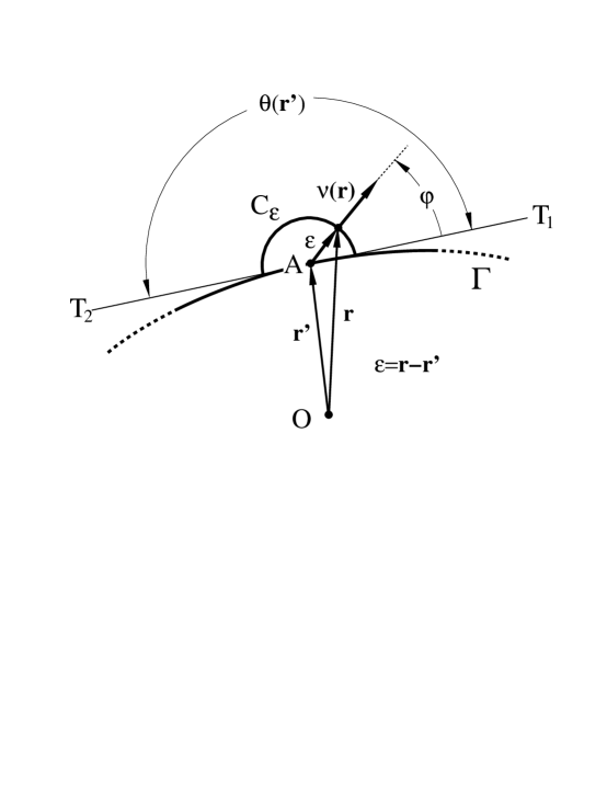
Fig. 1.: Geometry of the boundary $\Gamma_{\varepsilon}$ in the vicinity of the point A (position vector r’) where the Green’s function is singular.

The integration along $\tilde{\Gamma}_{\varepsilon}$ in the $\varepsilon\rightarrow 0^{+}$ limit is, by definition, Cauchy’s principal value integral along the original contour $\Gamma$. We denote the integral as

$$\lim_{\varepsilon\rightarrow 0}\int_{\Gamma_{\varepsilon}}\!ds(\mathchoice{{\hbox{\boldmath$\displaystyle r$}}}{{\hbox{\boldmath$\textstyle r$}}}{{\hbox{\boldmath$\scriptstyle r$}}}{{\hbox{\boldmath$\scriptscriptstyle r$}}})\ldots\equiv{\cal P}\oint_{\Gamma}\!ds(\mathchoice{{\hbox{\boldmath$\displaystyle r$}}}{{\hbox{\boldmath$\textstyle r$}}}{{\hbox{\boldmath$\scriptstyle r$}}}{{\hbox{\boldmath$\scriptscriptstyle r$}}})\ldots\;.$$ (13)

The contribution due to the integral along $C_{\varepsilon}$ depends on the type of singularity of the Green’s function at $\mathchoice{{\hbox{\boldmath$\displaystyle r$}}}{{\hbox{\boldmath$\textstyle r$}}}{{\hbox{\boldmath$\scriptstyle r$}}}{{\hbox{\boldmath$\scriptscriptstyle r$}}}=\mathchoice{{\hbox{\boldmath$\displaystyle r^{\prime}$}}}{{\hbox{\boldmath$\textstyle r^{\prime}$}}}{{\hbox{\boldmath$\scriptstyle r^{\prime}$}}}{{\hbox{\boldmath$\scriptscriptstyle r^{\prime}$}}}$. The integral can be calculated as shown in Appendix B. One obtains

$$lim_{\varepsilon\rightarrow 0}\frac{\hbar^{2}}{2m}\int_{C_{\varepsilon}}\!ds(\mathchoice{{\hbox{\boldmath$\displaystyle r$}}}{{\hbox{\boldmath$\textstyle r$}}}{{\hbox{\boldmath$\scriptstyle r$}}}{{\hbox{\boldmath$\scriptscriptstyle r$}}})\left[\psi_{n}(\mathchoice{{\hbox{\boldmath$\displaystyle r$}}}{{\hbox{\boldmath$\textstyle r$}}}{{\hbox{\boldmath$\scriptstyle r$}}}{{\hbox{\boldmath$\scriptscriptstyle r$}}})\partial_{\nu}G\left(\mathchoice{{\hbox{\boldmath$\displaystyle r$}}}{{\hbox{\boldmath$\textstyle r$}}}{{\hbox{\boldmath$\scriptstyle r$}}}{{\hbox{\boldmath$\scriptscriptstyle r$}}},\mathchoice{{\hbox{\boldmath$\displaystyle r^{\prime}$}}}{{\hbox{\boldmath$\textstyle r^{\prime}$}}}{{\hbox{\boldmath$\scriptstyle r^{\prime}$}}}{{\hbox{\boldmath$\scriptscriptstyle r^{\prime}$}}};E_{n}\right)-G\left(\mathchoice{{\hbox{\boldmath$\displaystyle r$}}}{{\hbox{\boldmath$\textstyle r$}}}{{\hbox{\boldmath$\scriptstyle r$}}}{{\hbox{\boldmath$\scriptscriptstyle r$}}},\mathchoice{{\hbox{\boldmath$\displaystyle r^{\prime}$}}}{{\hbox{\boldmath$\textstyle r^{\prime}$}}}{{\hbox{\boldmath$\scriptstyle r^{\prime}$}}}{{\hbox{\boldmath$\scriptscriptstyle r^{\prime}$}}};E_{n}\right)\partial_{\nu}\psi_{n}(\mathchoice{{\hbox{\boldmath$\displaystyle r$}}}{{\hbox{\boldmath$\textstyle r$}}}{{\hbox{\boldmath$\scriptstyle r$}}}{{\hbox{\boldmath$\scriptscriptstyle r$}}})\right]\;=\;\frac{1}{2}\psi_{n}(\mathchoice{{\hbox{\boldmath$\displaystyle r^{\prime}$}}}{{\hbox{\boldmath$\textstyle r^{\prime}$}}}{{\hbox{\boldmath$\scriptstyle r^{\prime}$}}}{{\hbox{\boldmath$\scriptscriptstyle r^{\prime}$}}})\;.$$ (14)

In the derivation of this formula we have implicitly assumed that there is a unique tangent to $\Gamma$ at $\textstyle r^{\prime}$, i.e., that the angle $\theta(\mathchoice{{\hbox{\boldmath$\displaystyle r$}}}{{\hbox{\boldmath$\textstyle r$}}}{{\hbox{\boldmath$\scriptstyle r$}}}{{\hbox{\boldmath$\scriptscriptstyle r$}}}^{\prime})$ in Fig. 1 is equal to $\pi$. Otherwise, according to Eq.(B5) in Appendix B, the RHS of (14) must be replaced by $\left(\theta(\mathchoice{{\hbox{\boldmath$\displaystyle r^{\prime}$}}}{{\hbox{\boldmath$\textstyle r^{\prime}$}}}{{\hbox{\boldmath$\scriptstyle r^{\prime}$}}}{{\hbox{\boldmath$\scriptscriptstyle r^{\prime}$}}})/2\pi\right)\psi_{n}(\mathchoice{{\hbox{\boldmath$\displaystyle r^{\prime}$}}}{{\hbox{\boldmath$\textstyle r^{\prime}$}}}{{\hbox{\boldmath$\scriptstyle r^{\prime}$}}}{{\hbox{\boldmath$\scriptscriptstyle r^{\prime}$}}})$, where $\theta(\mathchoice{{\hbox{\boldmath$\displaystyle r^{\prime}$}}}{{\hbox{\boldmath$\textstyle r^{\prime}$}}}{{\hbox{\boldmath$\scriptstyle r^{\prime}$}}}{{\hbox{\boldmath$\scriptscriptstyle r^{\prime}$}}})$ is the exterior angle between the two tangents to $\Gamma$ at $\textstyle r^{\prime}$.

Altogether, one obtains for $\psi_{n}(\mathchoice{{\hbox{\boldmath$\displaystyle r^{\prime}$}}}{{\hbox{\boldmath$\textstyle r^{\prime}$}}}{{\hbox{\boldmath$\scriptstyle r^{\prime}$}}}{{\hbox{\boldmath$\scriptscriptstyle r^{\prime}$}}})$ , $\mathchoice{{\hbox{\boldmath$\displaystyle r^{\prime}$}}}{{\hbox{\boldmath$\textstyle r^{\prime}$}}}{{\hbox{\boldmath$\scriptstyle r^{\prime}$}}}{{\hbox{\boldmath$\scriptscriptstyle r^{\prime}$}}}\,\in\,\Gamma$ the integral equation

$$\psi_{n}(\mathchoice{{\hbox{\boldmath$\displaystyle r^{\prime}$}}}{{\hbox{\boldmath$\textstyle r^{\prime}$}}}{{\hbox{\boldmath$\scriptstyle r^{\prime}$}}}{{\hbox{\boldmath$\scriptscriptstyle r^{\prime}$}}})\;=\;\frac{\hbar^{2}}{m}{\cal P}\oint_{\Gamma}\!ds(\mathchoice{{\hbox{\boldmath$\displaystyle r$}}}{{\hbox{\boldmath$\textstyle r$}}}{{\hbox{\boldmath$\scriptstyle r$}}}{{\hbox{\boldmath$\scriptscriptstyle r$}}})\left[\psi_{n}(\mathchoice{{\hbox{\boldmath$\displaystyle r$}}}{{\hbox{\boldmath$\textstyle r$}}}{{\hbox{\boldmath$\scriptstyle r$}}}{{\hbox{\boldmath$\scriptscriptstyle r$}}})\partial_{\nu}G\left(\mathchoice{{\hbox{\boldmath$\displaystyle r$}}}{{\hbox{\boldmath$\textstyle r$}}}{{\hbox{\boldmath$\scriptstyle r$}}}{{\hbox{\boldmath$\scriptscriptstyle r$}}},\mathchoice{{\hbox{\boldmath$\displaystyle r^{\prime}$}}}{{\hbox{\boldmath$\textstyle r^{\prime}$}}}{{\hbox{\boldmath$\scriptstyle r^{\prime}$}}}{{\hbox{\boldmath$\scriptscriptstyle r^{\prime}$}}};E_{n}\right)-G\left(\mathchoice{{\hbox{\boldmath$\displaystyle r$}}}{{\hbox{\boldmath$\textstyle r$}}}{{\hbox{\boldmath$\scriptstyle r$}}}{{\hbox{\boldmath$\scriptscriptstyle r$}}},\mathchoice{{\hbox{\boldmath$\displaystyle r^{\prime}$}}}{{\hbox{\boldmath$\textstyle r^{\prime}$}}}{{\hbox{\boldmath$\scriptstyle r^{\prime}$}}}{{\hbox{\boldmath$\scriptscriptstyle r^{\prime}$}}};E_{n}\right)\partial_{\nu}\psi_{n}(\mathchoice{{\hbox{\boldmath$\displaystyle r$}}}{{\hbox{\boldmath$\textstyle r$}}}{{\hbox{\boldmath$\scriptstyle r$}}}{{\hbox{\boldmath$\scriptscriptstyle r$}}})\right]$$ (15)

where one still needs to specify the boundary condition on $\Gamma$ which involves $\psi_{n}$ and/or its normal derivative $\partial_{\nu}\psi_{n}$. The boundary condition is expressed as a linear functional relation

$${\cal F}\left[\psi_{n}(\mathchoice{{\hbox{\boldmath$\displaystyle r$}}}{{\hbox{\boldmath$\textstyle r$}}}{{\hbox{\boldmath$\scriptstyle r$}}}{{\hbox{\boldmath$\scriptscriptstyle r$}}}),\partial_{\nu}\psi_{n}(\mathchoice{{\hbox{\boldmath$\displaystyle r$}}}{{\hbox{\boldmath$\textstyle r$}}}{{\hbox{\boldmath$\scriptstyle r$}}}{{\hbox{\boldmath$\scriptscriptstyle r$}}})\right]\;=\;0\;,\qquad\mathchoice{{\hbox{\boldmath$\displaystyle r$}}}{{\hbox{\boldmath$\textstyle r$}}}{{\hbox{\boldmath$\scriptstyle r$}}}{{\hbox{\boldmath$\scriptscriptstyle r$}}}\in\Gamma\;.$$ (16)

The actual form of the functional ${\cal F}$ depends on the physical problem at hand, but not on the contour $\Gamma$. The energy eigenvalues $E_{n}$ are determined by requiring that Eqs.(15) and (16) admit nontrivial solutions for $\psi_{n}$. This condition leads us to an equation involving functional (Fredholm) determinants of the type (5) which need to be solved by numerical means. Once $E_{n}$ and the corresponding $\psi_{n}$ and $\partial_{\nu}\psi_{n}$ on $\Gamma$ are determined, the eigenfunction inside the domain ${\cal D}$ can be calculated using Eq.(11).

Below we will demonstrate the application of the method outlined which is referred to as the Boundary Integral Method (BIM). The method is practical whenever (i) a Green’s function $G$ is available analytically and (ii) the boundary condition (16) is fairly simple; the method applies to $\Gamma$ of arbitrary shape.

III Billiard Spectra via BIM

Inside a billiard a particle moves freely, i.e., $V\,\equiv\,0$ in (6). The Green’s function defined through (7) is well known in this case and is given by

$$G\left(\mathchoice{{\hbox{\boldmath$\displaystyle r$}}}{{\hbox{\boldmath$\textstyle r$}}}{{\hbox{\boldmath$\scriptstyle r$}}}{{\hbox{\boldmath$\scriptscriptstyle r$}}},\mathchoice{{\hbox{\boldmath$\displaystyle r^{\prime}$}}}{{\hbox{\boldmath$\textstyle r^{\prime}$}}}{{\hbox{\boldmath$\scriptstyle r^{\prime}$}}}{{\hbox{\boldmath$\scriptscriptstyle r^{\prime}$}}};E\right)\;=\;-\frac{im}{2\hbar^{2}}H_{0}^{(1)}\left(k\left|\mathchoice{{\hbox{\boldmath$\displaystyle r$}}}{{\hbox{\boldmath$\textstyle r$}}}{{\hbox{\boldmath$\scriptstyle r$}}}{{\hbox{\boldmath$\scriptscriptstyle r$}}}-\mathchoice{{\hbox{\boldmath$\displaystyle r^{\prime}$}}}{{\hbox{\boldmath$\textstyle r^{\prime}$}}}{{\hbox{\boldmath$\scriptstyle r^{\prime}$}}}{{\hbox{\boldmath$\scriptscriptstyle r^{\prime}$}}}\right|\right)\;,$$ (17)

as shown in Appendix A. Here $k=\sqrt{2mE}/\hbar$ is the so-called wave vector; the index $n$ is dropped since we focus in the following on a single eigenstate. We will also use the notation $G\left(\mathchoice{{\hbox{\boldmath$\displaystyle r$}}}{{\hbox{\boldmath$\textstyle r$}}}{{\hbox{\boldmath$\scriptstyle r$}}}{{\hbox{\boldmath$\scriptscriptstyle r$}}},\mathchoice{{\hbox{\boldmath$\displaystyle r^{\prime}$}}}{{\hbox{\boldmath$\textstyle r^{\prime}$}}}{{\hbox{\boldmath$\scriptstyle r^{\prime}$}}}{{\hbox{\boldmath$\scriptscriptstyle r^{\prime}$}}};k\right)$ for the Green’s function. Since the particle is confined to the billiard, its wave function $\psi\equiv\psi_{n}$ must vanish along $\Gamma$ and the boundary condition (16) takes the form

$$\psi(\mathchoice{{\hbox{\boldmath$\displaystyle r$}}}{{\hbox{\boldmath$\textstyle r$}}}{{\hbox{\boldmath$\scriptstyle r$}}}{{\hbox{\boldmath$\scriptscriptstyle r$}}})\;=\;0\;,\quad\partial_{\nu}\psi(\mathchoice{{\hbox{\boldmath$\displaystyle r$}}}{{\hbox{\boldmath$\textstyle r$}}}{{\hbox{\boldmath$\scriptstyle r$}}}{{\hbox{\boldmath$\scriptscriptstyle r$}}})\;=\;\text{arbitrary}\;,\qquad\forall\>\mathchoice{{\hbox{\boldmath$\displaystyle r$}}}{{\hbox{\boldmath$\textstyle r$}}}{{\hbox{\boldmath$\scriptstyle r$}}}{{\hbox{\boldmath$\scriptscriptstyle r$}}}\in\Gamma\;.$$ (18)

Inserting (18) in the the integral equation (15) leads to

$${\cal P}\oint_{\Gamma}\!ds(\mathchoice{{\hbox{\boldmath$\displaystyle r$}}}{{\hbox{\boldmath$\textstyle r$}}}{{\hbox{\boldmath$\scriptstyle r$}}}{{\hbox{\boldmath$\scriptscriptstyle r$}}})G\left(\mathchoice{{\hbox{\boldmath$\displaystyle r$}}}{{\hbox{\boldmath$\textstyle r$}}}{{\hbox{\boldmath$\scriptstyle r$}}}{{\hbox{\boldmath$\scriptscriptstyle r$}}},\mathchoice{{\hbox{\boldmath$\displaystyle r^{\prime}$}}}{{\hbox{\boldmath$\textstyle r^{\prime}$}}}{{\hbox{\boldmath$\scriptstyle r^{\prime}$}}}{{\hbox{\boldmath$\scriptscriptstyle r^{\prime}$}}};E\right)\partial_{\nu}\psi(\mathchoice{{\hbox{\boldmath$\displaystyle r$}}}{{\hbox{\boldmath$\textstyle r$}}}{{\hbox{\boldmath$\scriptstyle r$}}}{{\hbox{\boldmath$\scriptscriptstyle r$}}})\;=\;0\;.$$ (19)

This integral equation admits non-trivial solutions only if the corresponding Fredholm (functional) determinant vanishes, i.e., for

$$\text{det}\left[G\left(\mathchoice{{\hbox{\boldmath$\displaystyle r$}}}{{\hbox{\boldmath$\textstyle r$}}}{{\hbox{\boldmath$\scriptstyle r$}}}{{\hbox{\boldmath$\scriptscriptstyle r$}}},\mathchoice{{\hbox{\boldmath$\displaystyle r^{\prime}$}}}{{\hbox{\boldmath$\textstyle r^{\prime}$}}}{{\hbox{\boldmath$\scriptstyle r^{\prime}$}}}{{\hbox{\boldmath$\scriptscriptstyle r^{\prime}$}}};E\right)\right]\;=\;0\;,$$ (20)

a condition which allows one to determine the energies $E_{n}$.

Even though the analytical expression of the Green’s function $G$ is known, the Fredholm determinant (20) is difficult to evaluate for arbitrary billiard boundaries $\Gamma$. Below we describe more practical schemes for solving the integral equation (19).

A Methods for Solving the BIE

There are basically three different methods for solving the BIE (15) for the billiard problem. Before presenting these methods, let us first parameterize the billiard boundary $\Gamma$ through the arc length $s\in[0,{\cal L}]$, where ${\cal L}$ is the length of the billiard boundary $\Gamma$. Thus, the position of each point $\mathchoice{{\hbox{\boldmath$\displaystyle r$}}}{{\hbox{\boldmath$\textstyle r$}}}{{\hbox{\boldmath$\scriptstyle r$}}}{{\hbox{\boldmath$\scriptscriptstyle r$}}}\in\Gamma$ is uniquely determined by $s$ through the function $\mathchoice{{\hbox{\boldmath$\displaystyle r$}}}{{\hbox{\boldmath$\textstyle r$}}}{{\hbox{\boldmath$\scriptstyle r$}}}{{\hbox{\boldmath$\scriptscriptstyle r$}}}=\mathchoice{{\hbox{\boldmath$\displaystyle r$}}}{{\hbox{\boldmath$\textstyle r$}}}{{\hbox{\boldmath$\scriptstyle r$}}}{{\hbox{\boldmath$\scriptscriptstyle r$}}}(s)$. It is convenient to introduce the notation

$$u(s)\equiv u_{n}(\mathchoice{{\hbox{\boldmath$\displaystyle r$}}}{{\hbox{\boldmath$\textstyle r$}}}{{\hbox{\boldmath$\scriptstyle r$}}}{{\hbox{\boldmath$\scriptscriptstyle r$}}}(s))\equiv\partial_{\nu}\psi_{n}(\mathchoice{{\hbox{\boldmath$\displaystyle r$}}}{{\hbox{\boldmath$\textstyle r$}}}{{\hbox{\boldmath$\scriptstyle r$}}}{{\hbox{\boldmath$\scriptscriptstyle r$}}})\;.$$ (21)

The BIE (19) can be recast then as

$$\int_{0}^{\cal L}\!ds\;G\left(s,s^{\prime};k\right)u(s)\;=\;0,$$ (22)

where, for brevity, we have dropped the index $n$ which labels the eigenstates.

Method I.    The most obvious (but not necessarily the most convenient) method of solution relies on the observation that both the wave function and its normal derivative (i.e., $u(s)$) are single-valued functions and, therefore, $u(s)$ must be a periodic function of $s$ with period ${\cal L}$. Hence, (22) can be expressed as a Fourier series

$$u(s)\;=\;\sum_{j=-\infty}^{\infty}u_{j}\exp(iK_{j}s)\;,$$ (24)

where

$$K_{j}\;\equiv\;\frac{2\pi}{{\cal L}}j\;,\qquad j=0,\pm 1,\pm 2,\ldots$$ (25)

and where $u_{j}$ is the Fourier transform of $u(s)$

$$u_{j}\;=\;\frac{1}{{\cal L}}\int_{0}^{\cal L}\!ds\,u(s)\exp(-iK_{j}s)\;.$$ (26)

By taking the Fourier transform of Eq.(22) with respect to $s^{\prime}$ and using (24) one obtains the system of linear equations

$$\sum_{j=-\infty}^{\infty}A_{ij}(k)\,u_{j}\;=\;0\;,$$ (27)

where

$$A_{ij}(k)\;=\;\frac{1}{{\cal L}}\int_{0}^{\cal L}\!ds\int_{0}^{\cal L}\!ds^{\prime}G\left(s,s^{\prime};k\right)\exp\left[-i(K_{i}s^{\prime}-K_{j}s)\right]\;.$$ (28)

Here the information about the billiard boundary $\Gamma$ is contained in the $s$- and $s^{\prime}$-dependence of the Green’s function through $\mathchoice{{\hbox{\boldmath$\displaystyle r$}}}{{\hbox{\boldmath$\textstyle r$}}}{{\hbox{\boldmath$\scriptstyle r$}}}{{\hbox{\boldmath$\scriptscriptstyle r$}}}=\mathchoice{{\hbox{\boldmath$\displaystyle r$}}}{{\hbox{\boldmath$\textstyle r$}}}{{\hbox{\boldmath$\scriptstyle r$}}}{{\hbox{\boldmath$\scriptscriptstyle r$}}}(s)$ and $\mathchoice{{\hbox{\boldmath$\displaystyle r^{\prime}$}}}{{\hbox{\boldmath$\textstyle r^{\prime}$}}}{{\hbox{\boldmath$\scriptstyle r^{\prime}$}}}{{\hbox{\boldmath$\scriptscriptstyle r^{\prime}$}}}=\mathchoice{{\hbox{\boldmath$\displaystyle r$}}}{{\hbox{\boldmath$\textstyle r$}}}{{\hbox{\boldmath$\scriptstyle r$}}}{{\hbox{\boldmath$\scriptscriptstyle r$}}}(s^{\prime})$. The energy eigenvalues, expressed through $k$, are the solutions of the equation

$$\text{det}\left[A_{ij}(k)\right]\;=\;0$$ (29)

which must hold in order to render (27) solvable.

For an arbitrary $\Gamma$ one cannot solve Eq.(29) exactly. However, approximate energy eigenvalues can be obtained by truncating the infinite system of linear equations (27) at some suitably chosen wave vector $K_{c}$. The truncation implies that the Fourier components of $u(s)$ which correspond to $|K_{j}|>K_{c}$ are set equal to zero in (24). In this case the relevant part of the matrix $A_{ij}$ becomes finite and the corresponding determinant can be calculated numerically. The drawback of the truncation is that the resulting energy eigenvalues expressed through $k$ are accurate only as long as $k\lesssim K_{c}$. If one seeks to describe energy levels with larger $k$-values one needs to increase $K_{c}$ which, however, leads to an increased computational effort, the latter increasing rapidly with the dimension of the matrix $A_{ij}$.

The calculation of the matrix elements $A_{ij}$ as double integrals (with an integrand which is singular at $s=s^{\prime}$) is computationally cumbersome and, as a result, the present method is impractical, except for the case of a circular billiard. In this case $A_{ij}(k)$ is a diagonal matrix and its elements can be expressed in terms of products of Bessel and Hankel functions as shown in Appendix C. Equation (29) reads then

$$\text{det}\left[A_{ij}(k)\right]\;\propto\;\prod_{j=-\infty}^{\infty}J_{j}(k)H_{j}^{(1)}(k)\;=\;0\;.$$ (30)

The Hankel functions $H_{j}^{(1)}(k)$ have no real roots and, hence, the energy eigenvalues for a circular billiard with unit radius are given by the zeros of the integer order Bessel functions

$$J_{j}\left(k_{n}\right)\;=\;0\;,\qquad E_{n}\;=\;\hbar^{2}k_{n}^{2}/2m\;,\qquad j=0,\pm 1,\pm 2,\ldots$$ (31)

a well known result, which can also be obtained by solving the Schrödinger equation (1) by means of separation of variables[8]. The present derivation of this result demonstrates the equivalence of the BIE (22) and the stationary Schrödinger equation. Note that because $J_{-j}(k)=(-1)^{j}J_{j}(k)$ [formula 9.1.5 in Ref.[23]] all the roots corresponding to $j\neq 0$ are doubly degenerate.

Method II.    Rather than approximating the BIE in Fourier space one can approximate it in coordinate space, i.e., one can solve (19) and not (27). For this purpose one proceeds in two steps. First, one approximates the boundary $\Gamma$ by a polygon with $N$ vertices situated on $\Gamma$, as shown in Fig. 2. Denoting the segment between vertices $i$ and $i+1$ by $\Gamma_{i}$ one can write $\Gamma\approx\cup_{i=1}^{N}\Gamma_{i}$, and the BIE can be approximated by a sum of integrals along the $N$ sides of the polygon. In a second step, one replaces along each segment $\Gamma_{i}$ the function $u(s)\equiv\partial_{\nu}\psi_{n}(\mathchoice{{\hbox{\boldmath$\displaystyle r$}}}{{\hbox{\boldmath$\textstyle r$}}}{{\hbox{\boldmath$\scriptstyle r$}}}{{\hbox{\boldmath$\scriptscriptstyle r$}}})$ by a constant $u_{i}$. The BIE is then replaced by

$$\sum_{i=1}^{N}u_{i}\int_{\Gamma_{i}}\!ds(\mathchoice{{\hbox{\boldmath$\displaystyle r$}}}{{\hbox{\boldmath$\textstyle r$}}}{{\hbox{\boldmath$\scriptstyle r$}}}{{\hbox{\boldmath$\scriptscriptstyle r$}}})\,G\left(\mathchoice{{\hbox{\boldmath$\displaystyle r$}}}{{\hbox{\boldmath$\textstyle r$}}}{{\hbox{\boldmath$\scriptstyle r$}}}{{\hbox{\boldmath$\scriptscriptstyle r$}}},\mathchoice{{\hbox{\boldmath$\displaystyle r^{\prime}$}}}{{\hbox{\boldmath$\textstyle r^{\prime}$}}}{{\hbox{\boldmath$\scriptstyle r^{\prime}$}}}{{\hbox{\boldmath$\scriptscriptstyle r^{\prime}$}}};k\right)\;=\;0\;.$$ (32)

Equation (32) still contains the continuous variable $\textstyle r^{\prime}$ which should be eliminated. For this purpose, let us denote the position vector of the vertex $i$ (see Fig.2) by $\mathchoice{{\hbox{\boldmath$\displaystyle s$}}}{{\hbox{\boldmath$\textstyle s$}}}{{\hbox{\boldmath$\scriptstyle s$}}}{{\hbox{\boldmath$\scriptscriptstyle s$}}}_{i}$ and the position vector of the middle point of $\Gamma_{i}$ by $\mathchoice{{\hbox{\boldmath$\displaystyle r$}}}{{\hbox{\boldmath$\textstyle r$}}}{{\hbox{\boldmath$\scriptstyle r$}}}{{\hbox{\boldmath$\scriptscriptstyle r$}}}_{i}=\left(\mathchoice{{\hbox{\boldmath$\displaystyle s$}}}{{\hbox{\boldmath$\textstyle s$}}}{{\hbox{\boldmath$\scriptstyle s$}}}{{\hbox{\boldmath$\scriptscriptstyle s$}}}_{i}+\mathchoice{{\hbox{\boldmath$\displaystyle s$}}}{{\hbox{\boldmath$\textstyle s$}}}{{\hbox{\boldmath$\scriptstyle s$}}}{{\hbox{\boldmath$\scriptscriptstyle s$}}}_{i+1}\right)/2$. Then, setting in (32) $\mathchoice{{\hbox{\boldmath$\displaystyle r^{\prime}$}}}{{\hbox{\boldmath$\textstyle r^{\prime}$}}}{{\hbox{\boldmath$\scriptstyle r^{\prime}$}}}{{\hbox{\boldmath$\scriptscriptstyle r^{\prime}$}}}=\mathchoice{{\hbox{\boldmath$\displaystyle r$}}}{{\hbox{\boldmath$\textstyle r$}}}{{\hbox{\boldmath$\scriptstyle r$}}}{{\hbox{\boldmath$\scriptscriptstyle r$}}}_{j}$, $j=1,2,\ldots,N$, one arrives at the so-called Boundary Element Equation (BEE)[9, 10]

$$\sum_{i=1}^{N}u_{i}\;\Delta{s}_{i}\!\int_{-\frac{1}{2}}^{\frac{1}{2}}\!d\xi\,G\left(\mathchoice{{\hbox{\boldmath$\displaystyle r$}}}{{\hbox{\boldmath$\textstyle r$}}}{{\hbox{\boldmath$\scriptstyle r$}}}{{\hbox{\boldmath$\scriptscriptstyle r$}}}_{i}+\xi\Delta\mathchoice{{\hbox{\boldmath$\displaystyle s$}}}{{\hbox{\boldmath$\textstyle s$}}}{{\hbox{\boldmath$\scriptstyle s$}}}{{\hbox{\boldmath$\scriptscriptstyle s$}}}_{i},\mathchoice{{\hbox{\boldmath$\displaystyle r$}}}{{\hbox{\boldmath$\textstyle r$}}}{{\hbox{\boldmath$\scriptstyle r$}}}{{\hbox{\boldmath$\scriptscriptstyle r$}}}_{j};k\right)\;=\;0\;,$$ (33)

where $\Delta\mathchoice{{\hbox{\boldmath$\displaystyle s$}}}{{\hbox{\boldmath$\textstyle s$}}}{{\hbox{\boldmath$\scriptstyle s$}}}{{\hbox{\boldmath$\scriptscriptstyle s$}}}_{i}\equiv\mathchoice{{\hbox{\boldmath$\displaystyle s$}}}{{\hbox{\boldmath$\textstyle s$}}}{{\hbox{\boldmath$\scriptstyle s$}}}{{\hbox{\boldmath$\scriptscriptstyle s$}}}_{i+1}-\mathchoice{{\hbox{\boldmath$\displaystyle s$}}}{{\hbox{\boldmath$\textstyle s$}}}{{\hbox{\boldmath$\scriptstyle s$}}}{{\hbox{\boldmath$\scriptscriptstyle s$}}}_{i}$. The above equation represents a homogeneous system of $N$ linear equations and can be written

$$\sum_{j=1}^{N}B_{ij}(k)\;u_{j}\;=\;0\;.$$ (34)

The elements of the matrix $B_{ij}(k)$, up to an irrelevant constant factor, are given by [cf. Eq.(17)]

$$B_{ij}(k)\;\equiv\;\Delta{s}_{j}\int_{-\frac{1}{2}}^{\frac{1}{2}}\!d\xi\,H_{0}^{(1)}\left(k\left|\mathchoice{{\hbox{\boldmath$\displaystyle r$}}}{{\hbox{\boldmath$\textstyle r$}}}{{\hbox{\boldmath$\scriptstyle r$}}}{{\hbox{\boldmath$\scriptscriptstyle r$}}}_{j}-\mathchoice{{\hbox{\boldmath$\displaystyle r$}}}{{\hbox{\boldmath$\textstyle r$}}}{{\hbox{\boldmath$\scriptstyle r$}}}{{\hbox{\boldmath$\scriptscriptstyle r$}}}_{i}+\xi\Delta\mathchoice{{\hbox{\boldmath$\displaystyle s$}}}{{\hbox{\boldmath$\textstyle s$}}}{{\hbox{\boldmath$\scriptstyle s$}}}{{\hbox{\boldmath$\scriptscriptstyle s$}}}_{j}\right|\right)\;.$$ (35)

In analogy to our previous approach, the (approximate) energy eigenvalues can be obtained (in terms of $k$) from

$$\text{det}[B_{ij}(k)]\;=\;0\;,$$ (36)

i.e., as the real roots of this equation.

Fig. 2.: The billiard boundary $\Gamma$ is approximated by a polygon with N vertices.

The matrix elements $B_{ij}$ in (35) are expressed as single integrals in contrast to the matrix elements $A_{ij}$ defined in (28) which are expressed in terms of double integrals. As a result, Method II is computationally less demanding than Method I, but has nevertheless two unfortunate features. First, the evaluation of the diagonal matrix elements $B_{ii}$ requires special integration technique due to the (integrable) singularity of the Green’s function at $\xi=0$. Second, in contrast to Method I where the truncation of the exact, infinite matrix $A_{ij}$ (defined in the Fourier space) provides us with a natural cutoff wave vector $K_{c}$, in case of Method II the relationship between a similar $K_{c}$ and the degree of discretization of the boundary (in real space) is less obvious.

It should be emphasized that truncation in Fourier space is not quite equivalent to truncation (discretization of the boundary) in real space[15]. As an empirical rule, if one wishes to calculate energy eigenvalues corresponding to $k\lesssim K_{c}$ accurately, one must take at least a few (about ten) discretization points for each section of the boundary of length equal to the corresponding de Broglie wave length $\lambda=2\pi/K_{c}$. Thus, the number of discretization points $N$ scales with the length ${\cal L}$ of the billiard boundary and the wave vector $K_{c}$ as follows

$$N\;\sim\;10\frac{{\cal L}}{\lambda}\;=\;\frac{10}{2\pi}\left(K_{c}{\cal L}\right)\;\sim\;K_{c}{\cal L}.$$ (37)

Accordingly, accurate calculations of energy eigenvalues corresponding to sufficiently large $k$ values require a large number of discretization points $N$ along the boundary $\Gamma$, a condition which leads to large matrices $B_{ij}$ and, since these matrices are dense, to undesirable computational efforts.

Method III.    The most widely used method for the evaluation of billiard spectra is based on a non-singular version of the BIE (19). A simple, but not entirely rigorous[17], derivation of this method applies the normal derivative operator $\partial_{\nu^{\prime}}=\mathchoice{{\hbox{\boldmath$\displaystyle\nu$}}}{{\hbox{\boldmath$\textstyle\nu$}}}{{\hbox{\boldmath$\scriptstyle\nu$}}}{{\hbox{\boldmath$\scriptscriptstyle\nu$}}}(\mathchoice{{\hbox{\boldmath$\displaystyle r^{\prime}$}}}{{\hbox{\boldmath$\textstyle r^{\prime}$}}}{{\hbox{\boldmath$\scriptstyle r^{\prime}$}}}{{\hbox{\boldmath$\scriptscriptstyle r^{\prime}$}}})\cdot\nabla_{r^{\prime}}$ to both sides of Eq.(15) which, according to definition (21) and with boundary condition (18) leads to

$$u\left(\mathchoice{{\hbox{\boldmath$\displaystyle r^{\prime}$}}}{{\hbox{\boldmath$\textstyle r^{\prime}$}}}{{\hbox{\boldmath$\scriptstyle r^{\prime}$}}}{{\hbox{\boldmath$\scriptscriptstyle r^{\prime}$}}}\right)\;=\;-\frac{\hbar^{2}}{m}\oint_{\Gamma}ds(\mathchoice{{\hbox{\boldmath$\displaystyle r$}}}{{\hbox{\boldmath$\textstyle r$}}}{{\hbox{\boldmath$\scriptstyle r$}}}{{\hbox{\boldmath$\scriptscriptstyle r$}}})\,\partial_{\nu^{\prime}}G\left(\mathchoice{{\hbox{\boldmath$\displaystyle r$}}}{{\hbox{\boldmath$\textstyle r$}}}{{\hbox{\boldmath$\scriptstyle r$}}}{{\hbox{\boldmath$\scriptscriptstyle r$}}},\mathchoice{{\hbox{\boldmath$\displaystyle r^{\prime}$}}}{{\hbox{\boldmath$\textstyle r^{\prime}$}}}{{\hbox{\boldmath$\scriptstyle r^{\prime}$}}}{{\hbox{\boldmath$\scriptscriptstyle r^{\prime}$}}};E\right)u(\mathchoice{{\hbox{\boldmath$\displaystyle r$}}}{{\hbox{\boldmath$\textstyle r$}}}{{\hbox{\boldmath$\scriptstyle r$}}}{{\hbox{\boldmath$\scriptscriptstyle r$}}})\;.$$ (38)

The integral kernel on the RHS, indeed, is non-singular at $\mathchoice{{\hbox{\boldmath$\displaystyle r$}}}{{\hbox{\boldmath$\textstyle r$}}}{{\hbox{\boldmath$\scriptstyle r$}}}{{\hbox{\boldmath$\scriptscriptstyle r$}}}=\mathchoice{{\hbox{\boldmath$\displaystyle r^{\prime}$}}}{{\hbox{\boldmath$\textstyle r^{\prime}$}}}{{\hbox{\boldmath$\scriptstyle r^{\prime}$}}}{{\hbox{\boldmath$\scriptscriptstyle r^{\prime}$}}}$. BIE (38) is a homogeneous integral equation with unknown $u(\mathchoice{{\hbox{\boldmath$\displaystyle r$}}}{{\hbox{\boldmath$\textstyle r$}}}{{\hbox{\boldmath$\scriptstyle r$}}}{{\hbox{\boldmath$\scriptscriptstyle r$}}})$; the energy eigenvalues $E$ are given by the zeros of the corresponding Fredholm determinant [cf. Eq.(20)], i.e., as the solutions of

$$\text{det}\left[\delta\left(\mathchoice{{\hbox{\boldmath$\displaystyle r$}}}{{\hbox{\boldmath$\textstyle r$}}}{{\hbox{\boldmath$\scriptstyle r$}}}{{\hbox{\boldmath$\scriptscriptstyle r$}}}-\mathchoice{{\hbox{\boldmath$\displaystyle r^{\prime}$}}}{{\hbox{\boldmath$\textstyle r^{\prime}$}}}{{\hbox{\boldmath$\scriptstyle r^{\prime}$}}}{{\hbox{\boldmath$\scriptscriptstyle r^{\prime}$}}}\right)+\frac{\hbar^{2}}{m}\partial_{\nu^{\prime}}G\left(\mathchoice{{\hbox{\boldmath$\displaystyle r$}}}{{\hbox{\boldmath$\textstyle r$}}}{{\hbox{\boldmath$\scriptstyle r$}}}{{\hbox{\boldmath$\scriptscriptstyle r$}}},\mathchoice{{\hbox{\boldmath$\displaystyle r^{\prime}$}}}{{\hbox{\boldmath$\textstyle r^{\prime}$}}}{{\hbox{\boldmath$\scriptstyle r^{\prime}$}}}{{\hbox{\boldmath$\scriptscriptstyle r^{\prime}$}}};E\right)\right]\;=\;0\;.$$ (39)

Taking into account the explicit form (17) of the free particle Green’s function, Eq. (38) can be written [cf. Eq.(B3)]

$$u\left(\mathchoice{{\hbox{\boldmath$\displaystyle r^{\prime}$}}}{{\hbox{\boldmath$\textstyle r^{\prime}$}}}{{\hbox{\boldmath$\scriptstyle r^{\prime}$}}}{{\hbox{\boldmath$\scriptscriptstyle r^{\prime}$}}}\right)\;=\;-\frac{ik}{2}\oint_{\Gamma}ds(\mathchoice{{\hbox{\boldmath$\displaystyle r$}}}{{\hbox{\boldmath$\textstyle r$}}}{{\hbox{\boldmath$\scriptstyle r$}}}{{\hbox{\boldmath$\scriptscriptstyle r$}}})\cos\phi\left(\mathchoice{{\hbox{\boldmath$\displaystyle r^{\prime}$}}}{{\hbox{\boldmath$\textstyle r^{\prime}$}}}{{\hbox{\boldmath$\scriptstyle r^{\prime}$}}}{{\hbox{\boldmath$\scriptscriptstyle r^{\prime}$}}},\mathchoice{{\hbox{\boldmath$\displaystyle r$}}}{{\hbox{\boldmath$\textstyle r$}}}{{\hbox{\boldmath$\scriptstyle r$}}}{{\hbox{\boldmath$\scriptscriptstyle r$}}}\right)H_{1}^{(1)}\!\left(k|\mathchoice{{\hbox{\boldmath$\displaystyle r^{\prime}$}}}{{\hbox{\boldmath$\textstyle r^{\prime}$}}}{{\hbox{\boldmath$\scriptstyle r^{\prime}$}}}{{\hbox{\boldmath$\scriptscriptstyle r^{\prime}$}}}-\mathchoice{{\hbox{\boldmath$\displaystyle r$}}}{{\hbox{\boldmath$\textstyle r$}}}{{\hbox{\boldmath$\scriptstyle r$}}}{{\hbox{\boldmath$\scriptscriptstyle r$}}}|\right)u(\mathchoice{{\hbox{\boldmath$\displaystyle r$}}}{{\hbox{\boldmath$\textstyle r$}}}{{\hbox{\boldmath$\scriptstyle r$}}}{{\hbox{\boldmath$\scriptscriptstyle r$}}})\;,$$ (40)

where

$$\cos\phi\left(\mathchoice{{\hbox{\boldmath$\displaystyle r^{\prime}$}}}{{\hbox{\boldmath$\textstyle r^{\prime}$}}}{{\hbox{\boldmath$\scriptstyle r^{\prime}$}}}{{\hbox{\boldmath$\scriptscriptstyle r^{\prime}$}}},\mathchoice{{\hbox{\boldmath$\displaystyle r$}}}{{\hbox{\boldmath$\textstyle r$}}}{{\hbox{\boldmath$\scriptstyle r$}}}{{\hbox{\boldmath$\scriptscriptstyle r$}}}\right)\;\equiv\;\mathchoice{{\hbox{\boldmath$\displaystyle\nu$}}}{{\hbox{\boldmath$\textstyle\nu$}}}{{\hbox{\boldmath$\scriptstyle\nu$}}}{{\hbox{\boldmath$\scriptscriptstyle\nu$}}}(\mathchoice{{\hbox{\boldmath$\displaystyle r^{\prime}$}}}{{\hbox{\boldmath$\textstyle r^{\prime}$}}}{{\hbox{\boldmath$\scriptstyle r^{\prime}$}}}{{\hbox{\boldmath$\scriptscriptstyle r^{\prime}$}}})\cdot\frac{\mathchoice{{\hbox{\boldmath$\displaystyle r^{\prime}$}}}{{\hbox{\boldmath$\textstyle r^{\prime}$}}}{{\hbox{\boldmath$\scriptstyle r^{\prime}$}}}{{\hbox{\boldmath$\scriptscriptstyle r^{\prime}$}}}-\mathchoice{{\hbox{\boldmath$\displaystyle r$}}}{{\hbox{\boldmath$\textstyle r$}}}{{\hbox{\boldmath$\scriptstyle r$}}}{{\hbox{\boldmath$\scriptscriptstyle r$}}}}{|\mathchoice{{\hbox{\boldmath$\displaystyle r^{\prime}$}}}{{\hbox{\boldmath$\textstyle r^{\prime}$}}}{{\hbox{\boldmath$\scriptstyle r^{\prime}$}}}{{\hbox{\boldmath$\scriptscriptstyle r^{\prime}$}}}-\mathchoice{{\hbox{\boldmath$\displaystyle r$}}}{{\hbox{\boldmath$\textstyle r$}}}{{\hbox{\boldmath$\scriptstyle r$}}}{{\hbox{\boldmath$\scriptscriptstyle r$}}}|}$$ (41)

is the cosine of the angle between the exterior normal vector to $\Gamma$ at $\textstyle r^{\prime}$ and the unit vector corresponding to $\mathchoice{{\hbox{\boldmath$\displaystyle r^{\prime}$}}}{{\hbox{\boldmath$\textstyle r^{\prime}$}}}{{\hbox{\boldmath$\scriptstyle r^{\prime}$}}}{{\hbox{\boldmath$\scriptscriptstyle r^{\prime}$}}}-\mathchoice{{\hbox{\boldmath$\displaystyle r$}}}{{\hbox{\boldmath$\textstyle r$}}}{{\hbox{\boldmath$\scriptstyle r$}}}{{\hbox{\boldmath$\scriptscriptstyle r$}}}$. Note that for $\mathchoice{{\hbox{\boldmath$\displaystyle r$}}}{{\hbox{\boldmath$\textstyle r$}}}{{\hbox{\boldmath$\scriptstyle r$}}}{{\hbox{\boldmath$\scriptscriptstyle r$}}}=\mathchoice{{\hbox{\boldmath$\displaystyle r^{\prime}$}}}{{\hbox{\boldmath$\textstyle r^{\prime}$}}}{{\hbox{\boldmath$\scriptstyle r^{\prime}$}}}{{\hbox{\boldmath$\scriptscriptstyle r^{\prime}$}}}$ the above scalar product vanishes and, actually, cancels the singularity due to the Hankel function in the integrand of the BIE (40).

For a billiard with arbitrary boundary, the above functional determinant cannot be calculated analytically and one needs to resort to a numerical solution. For this purpose, one employs the same strategy as in case of Method II. After discretizing the boundary $\Gamma$, one can replace the BIE (40) by the BEE [cf. Eq.(33)]

$$u_{j}\;=\;-\frac{ik}{2}\sum_{i=1}^{N}u_{i}\Delta s_{i}\int_{-\frac{1}{2}}^{\frac{1}{2}}d\xi\,\cos\phi\left(\mathchoice{{\hbox{\boldmath$\displaystyle r$}}}{{\hbox{\boldmath$\textstyle r$}}}{{\hbox{\boldmath$\scriptstyle r$}}}{{\hbox{\boldmath$\scriptscriptstyle r$}}}_{j},\mathchoice{{\hbox{\boldmath$\displaystyle r$}}}{{\hbox{\boldmath$\textstyle r$}}}{{\hbox{\boldmath$\scriptstyle r$}}}{{\hbox{\boldmath$\scriptscriptstyle r$}}}_{i}+\xi\Delta s_{i}\right)H_{1}^{(1)}\!\left(k\left|\mathchoice{{\hbox{\boldmath$\displaystyle r$}}}{{\hbox{\boldmath$\textstyle r$}}}{{\hbox{\boldmath$\scriptstyle r$}}}{{\hbox{\boldmath$\scriptscriptstyle r$}}}_{j}-\mathchoice{{\hbox{\boldmath$\displaystyle r$}}}{{\hbox{\boldmath$\textstyle r$}}}{{\hbox{\boldmath$\scriptstyle r$}}}{{\hbox{\boldmath$\scriptscriptstyle r$}}}_{i}-\xi\Delta\mathchoice{{\hbox{\boldmath$\displaystyle s$}}}{{\hbox{\boldmath$\textstyle s$}}}{{\hbox{\boldmath$\scriptstyle s$}}}{{\hbox{\boldmath$\scriptscriptstyle s$}}}_{i}\right|\right)\;,$$ (42)

where the notations are the same as in the case of Method II. Since the integrands on the RHS of the above equation are well behaved for all $i,j=1,2,\ldots,N$, one can approximate the corresponding integrals by the trapezoidal rule. As a result one obtains the system of linear equations

$$\sum_{j=1}^{N}C_{ij}(k)\,u_{j}\;=\;0,$$ (43)

where

$$C_{ij}(k)\;\equiv\;\delta_{ij}+\frac{ik}{2}\Delta s_{j}\cos\phi_{ij}H_{1}^{(1)}\!\left(kr_{ij}\right)\;,$$ (44)

$$\cos\phi_{ij}\;=\;\mathchoice{{\hbox{\boldmath$\displaystyle\nu$}}}{{\hbox{\boldmath$\textstyle\nu$}}}{{\hbox{\boldmath$\scriptstyle\nu$}}}{{\hbox{\boldmath$\scriptscriptstyle\nu$}}}_{i}\cdot\frac{\mathchoice{{\hbox{\boldmath$\displaystyle r$}}}{{\hbox{\boldmath$\textstyle r$}}}{{\hbox{\boldmath$\scriptstyle r$}}}{{\hbox{\boldmath$\scriptscriptstyle r$}}}_{ij}}{r_{ij}}\;,\qquad\mathchoice{{\hbox{\boldmath$\displaystyle r$}}}{{\hbox{\boldmath$\textstyle r$}}}{{\hbox{\boldmath$\scriptstyle r$}}}{{\hbox{\boldmath$\scriptscriptstyle r$}}}_{ij}\;=\;\mathchoice{{\hbox{\boldmath$\displaystyle r$}}}{{\hbox{\boldmath$\textstyle r$}}}{{\hbox{\boldmath$\scriptstyle r$}}}{{\hbox{\boldmath$\scriptscriptstyle r$}}}_{i}-\mathchoice{{\hbox{\boldmath$\displaystyle r$}}}{{\hbox{\boldmath$\textstyle r$}}}{{\hbox{\boldmath$\scriptstyle r$}}}{{\hbox{\boldmath$\scriptscriptstyle r$}}}_{j}\;.$$ (45)

The (approximate) energy eigenvalues can be determined as the roots of the determinant of $C_{ij}$

$$\text{det}\left[C_{ij}(k)\right]\;=\;0\;.$$ (46)

B Numerical Algorithm for Solving the BEE

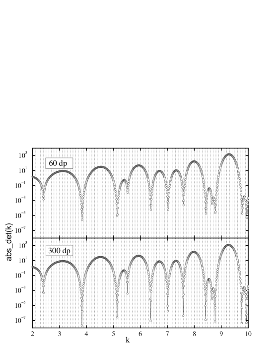
Fig. 3.: Plot of abs_det(k) (open circles) for the circle billiard, corresponding to 60 and 300 discretization points (dp) of the boundary, by using Method III. The positions of the minima approximate the sought eigenvalues $k_{n}$. While the values of the minima depend strongly on the degree of discretization of the boundary, the actual positions of the minima do not.

Based on the computational methods introduced we have written a FORTRAN 77 program which implements the necessary algorithmic steps using the SLATEC Common Mathematical Library[24]. For all three methods one can employ a common algorithmic framework containing (i) a function det($k$) which, for an input wave vector $k$, returns the complex value of the determinant of the corresponding system matrix, i.e., $A_{ij}$, $B_{ij}$ or $C_{ij}$; (ii) a routine solve which calculates approximately the roots of the equation det$(k)=0$. Once the function det$(k)$ and the corresponding root finder solve are available one can scan the interval of $k$ values of interest (between zero and the cut-off wave vector $K_{c}$) to determine the zeros $k_{n}$ of det$(k)$ and, hence, the energy eigenvalues $E_{n}$. The algorithm may fail in practice when the separation between two consecutive eigenvalues is smaller than the scanning step $\Delta k$, i.e., when eigenvalues are nearly degenerate. The only way to avoid this error is to use the smallest affordable $\Delta k$.

TABLE I.: The first 18 distinct eigenvalues $k_{n}$ corresponding to the circle billiard of unit radius obtained by using Methods I, II and III. The eigenvalues corresponding to Method I represent the zeros of the integer Bessel functions $J_{j}(k)$ and should be regarded as exact solutions. In case of Method II (III) the boundary was discretized by employing 60 (300) equally spaced points along the circle. The relative error for each approximate solution is less than 0.1%.

Method I	Method II	Method III		Method I	Method II	Method III
2.40482	2.4077	2.4053		8.77148	8.7800	8.7720
3.83170	3.8360	3.8320		9.76102	9.7720	9.7615
5.13562	5.1415	5.1360		9.93611	9.9440	9.9375
5.52007	5.5265	5.5206		10.17347	10.1855	10.1745
6.38016	6.3871	6.3806		11.06471	11.0760	11.0655
7.01558	7.0233	7.0160		11.08637	11.0945	11.0865
7.58834	7.5960	7.5888		11.61984	11.6335	11.6200
8.41724	8.4265	8.4175		11.79153	11.8055	11.7920
8.65372	8.6640	8.6545		12.22509	12.2320	12.2265

The actual form of det$(k)$ depends on the method chosen. In case of Method I, each matrix element $A_{ij}$ is given by a two-dimensional integral [see Eq.(28)] with singular and oscillatory integrand such that the evaluation of det$(k)$ would be computationally extremely demanding and would require special integration routines. Hence, we did not pursue an implementation of det$(k)$ for Method I. In the case of Methods II and III the function det$(k)$ consists of the following three parts

• The subroutine discretize which takes as input the data necessary to define the actual form of the billiard boundary and the number of discretization points $N$ of the billiard boundary; discretize returns as output the vectors $\mathchoice{{\hbox{\boldmath$\displaystyle r$}}}{{\hbox{\boldmath$\textstyle r$}}}{{\hbox{\boldmath$\scriptstyle r$}}}{{\hbox{\boldmath$\scriptscriptstyle r$}}}_{i}$, $\mathchoice{{\hbox{\boldmath$\displaystyle s$}}}{{\hbox{\boldmath$\textstyle s$}}}{{\hbox{\boldmath$\scriptstyle s$}}}{{\hbox{\boldmath$\scriptscriptstyle s$}}}_{i}$ ($i=1,\ldots,N$) [see Fig. 2] and other useful quantities based on them, such as the matrix $\mathchoice{{\hbox{\boldmath$\displaystyle r$}}}{{\hbox{\boldmath$\textstyle r$}}}{{\hbox{\boldmath$\scriptstyle r$}}}{{\hbox{\boldmath$\scriptscriptstyle r$}}}_{ij}=\mathchoice{{\hbox{\boldmath$\displaystyle r$}}}{{\hbox{\boldmath$\textstyle r$}}}{{\hbox{\boldmath$\scriptstyle r$}}}{{\hbox{\boldmath$\scriptscriptstyle r$}}}_{i}-\mathchoice{{\hbox{\boldmath$\displaystyle r$}}}{{\hbox{\boldmath$\textstyle r$}}}{{\hbox{\boldmath$\scriptstyle r$}}}{{\hbox{\boldmath$\scriptscriptstyle r$}}}_{j}$, the vectors $\Delta\mathchoice{{\hbox{\boldmath$\displaystyle s$}}}{{\hbox{\boldmath$\textstyle s$}}}{{\hbox{\boldmath$\scriptstyle s$}}}{{\hbox{\boldmath$\scriptscriptstyle s$}}}_{i}=\mathchoice{{\hbox{\boldmath$\displaystyle s$}}}{{\hbox{\boldmath$\textstyle s$}}}{{\hbox{\boldmath$\scriptstyle s$}}}{{\hbox{\boldmath$\scriptscriptstyle s$}}}_{i+1}-\mathchoice{{\hbox{\boldmath$\displaystyle s$}}}{{\hbox{\boldmath$\textstyle s$}}}{{\hbox{\boldmath$\scriptstyle s$}}}{{\hbox{\boldmath$\scriptscriptstyle s$}}}_{i}$, $\Delta s_{i}=|\Delta\mathchoice{{\hbox{\boldmath$\displaystyle s$}}}{{\hbox{\boldmath$\textstyle s$}}}{{\hbox{\boldmath$\scriptstyle s$}}}{{\hbox{\boldmath$\scriptscriptstyle s$}}}_{i}|$, $\mathchoice{{\hbox{\boldmath$\displaystyle\nu$}}}{{\hbox{\boldmath$\textstyle\nu$}}}{{\hbox{\boldmath$\scriptstyle\nu$}}}{{\hbox{\boldmath$\scriptscriptstyle\nu$}}}_{i}=\hat{\mathchoice{{\hbox{\boldmath$\displaystyle z$}}}{{\hbox{\boldmath$\textstyle z$}}}{{\hbox{\boldmath$\scriptstyle z$}}}{{\hbox{\boldmath$\scriptscriptstyle z$}}}}\times\Delta\mathchoice{{\hbox{\boldmath$\displaystyle s$}}}{{\hbox{\boldmath$\textstyle s$}}}{{\hbox{\boldmath$\scriptstyle s$}}}{{\hbox{\boldmath$\scriptscriptstyle s$}}}_{i}/\Delta s_{i}$ (i.e., the external unit vector to the boundary at $\mathchoice{{\hbox{\boldmath$\displaystyle r$}}}{{\hbox{\boldmath$\textstyle r$}}}{{\hbox{\boldmath$\scriptstyle r$}}}{{\hbox{\boldmath$\scriptscriptstyle r$}}}_{i}$), etc. If one does not want to change the degree of discretization of the billiard boundary during the successive evaluations of det$(k)$, subroutine discretize should be run only once, namely during the first call of the function det$(k)$.

• The subroutine sys_mat which evaluates the complex valued matrix elements $B_{ij}$ and $C_{ij}$ in case of Method II and III, respectively. The $B_{ij}$ are evaluated according to Eq.(35) employing two SLATEC[24] (more precisely QUADPACK[24]) quadrature routines, namely DQAGS, for calculating the non-diagonal matrix elements, and DQAWS, for calculating the diagonal matrix elements in which the integrand has a logarithmic singularity at $\xi=0$. The $C_{ij}$ are evaluated according to Eqs.(44-45) in a straightforward way. In both cases the Hankel functions can be expressed in terms of the corresponding Bessel and Neumann functions for which the double precision SLATEC routines DBESJ0, DBESJ1 and DBESY0, DBESY1, respectively, are called.

• The function det$(k)$ which evaluates the determinant of $B_{ij}$ and $C_{ij}$, respectively. For this purpose one employs the SLATEC subroutines[24] ZGEFA (factors a complex matrix by using Gaussian elimination) and ZGEDI (calculates the determinant and the inverse of a complex matrix by using the factors from ZGEFA).

The function det$(k)$ is complex-valued and, therefore, its real roots $k_{n}$ (the sought eigenvalues) must be simultaneously zeros of both real and imaginary parts of this function. Due to the finite discretization of the boundary, the numerical solutions of the equation det$(k)=0$ will be complex with a (hopefully) small imaginary part. In fact, the magnitude of the imaginary part of the “complex eigenvalue” $\tilde{k}_{n}$ can be used to characterize the accuracy of the energy eigenvalues thus determined through the real part of $\tilde{k}_{n}$. To the best of our knowledge, there exists no public domain subroutine which calculates automatically the roots of an arbitrary complex function of one complex variable, and as a result one can make little or no progress at all in the endeavor of constructing a robust $k_{n}$ eigenvalue finder algorithm based on the above straightforward approach. However, there is a relatively simple solution to this problem which seems to be widely used by practitioners of the BIM[11, 21]. One notes that the zeros of det$(k)$ are also absolute minima for the square of the absolute value of this function, i.e., of abs_det$(k)\equiv\text{Re}[\text{\tt det}(k)]^{2}+\text{Im}[\text{\tt det}(k)]^{2}$. Strictly speaking, the minima should assume zero values. The discretization of the boundary (or equivalently, the truncation of the original functional determinant) introduces errors such that the numerically evaluated minima of abs_det$(k)$, are small, but not zero; the magnitude of each minimum can be used to distinguish a real root of det$(k)$ from a local minimum of abs_det$(k)$. Since, numerically, it is much easier to determine the (local) minima of a real function of a real variable than to determine the roots of a complex function of a complex variable the suggested approach is much more convenient for our purpose. Accordingly, solve determines actually the local minima of abs_det$(k)$ by going through a given interval of wave vectors $k_{min}\leq k\leq k_{max}$ in steps of $\Delta k$. Once a minimum is bracketed, its actual value can be calculated with any desired accuracy (for a given degree of discretization of the billiard boundary) by employing, for example, a double precision version of the function brent from Ref. [25].

C Numerical Results

As a test of the algorithms described in Sec. III B and their numerical implementation we determine the spectrum of a circular billiard. In this case Method I yields the exact energy eigenvalues $k_{n}$ [cf. Eq.(31)] as the roots of the integer Bessel functions (these roots are in fact tabulated; see, e.g., Ref. [23]). The first 18 distinct eigenvalues $k_{n}$ were also determined by means of Methods II and III described in Sec. III A and are compared in Table I with the results of Method I. In case of Method II (III) 60 (300) equally spaced discretization points of the circular boundary have been employed. The locations of the minima of the function abs_det(k) have been determined by scanning the $2\leq k\leq 13$ interval with a step $\Delta k=0.004$. Figure 3 illustrates the $k$-dependence of abs_det(k), evaluated in the framework of Method III for two different discretizations of the boundary. An increase of the number of discretization points from 60 to 300 changes significantly the values, but not the positions of the minima and, hence, does not affect significantly the values $k_{n}$.

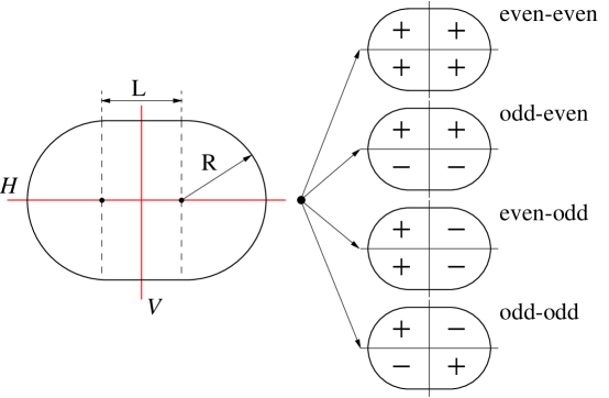
Fig. 4.: The stadium billiard is formed by two semicircles of radius R connected through two parallel linear segments of length L. The two symmetry axes of the stadium are labeled H (horizontal) and V (vertical), and the corresponding four symmetry classes of the energy eigenfunctions are shown.

Table I demonstrates that the results of both Methods II and III reproduce the exact eigenvalues to at least three significant digits for $k\lesssim K_{c}$ [cf. Eq.(37)]. In case of Method III, we have found that 300 discretization points lead to a precision of better than 1% for the 150 lowest eigenvalues of the circular billiard (with unit radius) corresponding to $k<35$. For larger $k$ values the density of eigenvalues increases and, in order to separate adjacent minima of abs_det(k), one needs to reduce the step size $\Delta k$. The method breaks down for $k\sim{\cal L}/N$, i.e., when the distance between two consecutive discretization points of the boundary becomes comparable with the de Broglie wavelength of the particle, and the only remedy is to increase $N$.

Fig. 5.: Spectral staircase $N(k)$ for the lowest 50 (70) energy levels of the (a) circle and (b) stadium billiard. In (a) the dashed line corresponds to the leading semiclassical Weyl term $(Sk^{2}/4\pi)/2$, where the extra factor of $1/2$ accounts for the double degeneracy of the energy eigenvalues with $m\neq 0$. The solid line is obtained by taking into account the perimeter (next to the leading) term in the Weyl formula which for the circle billiard is given by $\Delta N=k/4$. In (b) the solid line corresponds to the asymptotic Weyl formula with the perimeter correction term.

The program implementing Methods II, III allows one to calculate the spectra of billiards of arbitrary shapes, for which purpose one needs to solely alter the coordinates of the discretization points of the billiard boundary. As an example, we choose the Bunimovich stadium billiard depicted in Fig. 4 which consist of two semi-circles (of radius $R=1$) connected by two parallel linear segments (of length $L$) . We seek to calculate the lowest few hundred energy eigenvalues of both the circle and the stadium billiard.

The circle billiard constitutes an integrable system, i.e., the number of constants of motion (energy and angular momentum) is equal to the number of degrees of freedom . Its energy eigenstates can be classified according to symmetry, i.e., by an orbital quantum number $m$, which counts the nodal lines through the center, and a principal quantum number $n$, which counts the nodes of the radial wave function, i.e., the nodal circles[8]. In contrast, the stadium billiard, regardless of how small $L$ is, constitutes a non-integrable, i.e., (strongly) chaotic, system[4, 27]. The study of quantum systems for which the underlying classical motion is chaotic is a relatively new and still widely open field of study[28, 29]. Since it is beyond the scope of the present article to provide an introduction to quantum chaos, we will content ourselves with considering without explanation one characteristic which distinguishes the spectra of non-chaotic (e.g., of a circle billiard) and of chaotic (e.g., of a stadium billiard) quantum systems, namely the so called (energy) level spacing distribution $P(s)$. By definition[30, 31], $P(s)ds$ is the probability that, given an energy level at $E$, the nearest neighbor energy level is located in the interval $ds$ about $E+s$. According to Random Matrix Theory[31, 32] (RMT), applicable due to a quasi-random character of the Hamiltonian matrix, quantum systems, as far as the statistics of their energy spectrum is concerned, in general can be classified into four universality classes, with well defined and distinct $P(s)$ level spacing distributions[30, 31]. Integrable systems are described by the Poisson distribution with

$$P_{o}(s)\;=\;e^{-s}\;.$$ (47)

The energy levels of classically chaotic systems, which do not break time reversal symmetry, (e.g., the stadium billiard) form a Gaussian Orthogonal Ensemble (GOE) with

$$P_{GOE}(s)\;=\;\frac{\pi}{2}s\exp\left(-\frac{\pi s^{2}}{4}\right)\;.$$ (48)

Further universality classes are the Gaussian Unitary Ensemble (GUE) and the Gaussian Symplectic Ensemble (GSE); classical chaotic systems which break time reversal symmetry, e.g., ellipse or stadium billiards in an external magnetic field, belong to the GUE, while classical chaotic systems which preserve time reversal symmetry, but break spin rotational symmetry, e.g., a chaotic billiard in the presence of spin-orbit interaction, belong to the GSE.

Fig. 6.: Histogram of the energy level spacing distribution $P(s)$ for the (a) circle and (b) stadium billiards. In (a) the histogram is constructed from the lowest 1,200 energy levels of the circle billiard. The solid line corresponds to the Poisson prediction for the level spacing distribution. In (b) the lowest 600 energy levels have been used to construct the histogram. The dotted (dashed) line represents the Poisson (GOE) prediction for $P(s)$. The histogram is best approximated by the superposition of 4 independent GOE distributions (solid line) which correspond to the same number of distinct symmetry classes of the energy eigenstates in a stadium billiard.

Fig. 7.: Histogram of the energy level spacing distribution $P(s)$ for the (a) quarter- and (b) half-stadium billiards. The level spacing distribution for a quarter- (half-) stadium is well approximated by the GOE (two independent sequences of GOE) distribution function.

Poisson and GOE distributions are distinguished most clearly near $s=0$, since $P_{o}(0)=1$ constitutes the maximum of $P_{o}$ while $P_{GOE}(0)=0$ constitutes the minimum of $P_{GOE}$; neighboring energy levels are likely to attract (repel) each other in the case of integrable (chaotic) systems. We want to show that the level spacing distribution evaluated by means of the BIM for circle and stadium billiards satisfies the Poisson and GOE distribution, respectively. For this purpose one needs to calculate at least a few hundred of the lowest energy levels without actually missing any energy levels since such misses would distort the energy level spacing distribution. The quality of the calculations, in particular in the case of the stadium billiard, can be judged from a comparison of the obtained (energy) staircase function ${\cal N}(E)$ (which gives the number of quantum states with energy less or equal to $E$) with the corresponding Weyl-type formula[31, 33]

$$\langle{\cal N}(E)\rangle\;=\;\frac{1}{4\pi}\left(S\,E-{\cal L}\,\sqrt{E}+C\right)\;,$$ (49)

where $S$ and ${\cal L}$ are the area and perimeter of the billiard, and $C$ is a constant related to the geometry and topology of the billiard boundary. Presently, we employ units in which $\hbar^{2}/2m$ is equal to one; thus, e.g., $E=k^{2}$. Also, in the numerical results reported below we have chosen $L=R=1$ (see Fig. 4).

Strictly speaking Eq.(49) is valid only in the semi-classical ($E\rightarrow\infty$) limit, but in practice it turns out that one can apply Weyl’s formula even at the lower end of the energy spectrum. Our results for the staircase function ${\cal N}(k)$, corresponding to the first 50 (70) distinct energy levels of the circle (stadium) billiard, are presented in Fig. 5. In the case of the circle billiard a complication arises due to the fact that all the energy levels with angular momentum $m\neq 0$ are doubly degenerate. A simple remedy to this problem is to assume that the fraction of energy levels corresponding to $m=0$ is negligible in comparison to those with $m\neq 0$, and that the double degeneracy can be accounted for by dividing the RHS of Eq.(49) by two.

Based on the good agreement between ${\cal N}(E)$ and $\langle{\cal N}(E)\rangle$ shown in Fig. 5, one may conclude that all energy levels have been accounted for. A similar analysis for the first 600 energy levels showed that at most a few percent of the energy levels might been missed. This conclusion is independent of the method chosen, i.e., of Methods II and III.

TABLE II.: Wave vector eigenvalues $k_{n}\;(<10)$ for (a) quarter-, (b) horizontal half-, (c) vertical half- and (d) full stadium billiards. The quarter stadium has only odd-odd energy eigenstates, the horizontal (vertical) half stadium has both odd-odd and odd-even (even-odd) eigenstates, while the full stadium has eigenstates which belong to all four symmetry classes. The symmetry of each eigenstate of the (full) stadium billiard can be identified based on this table as explained in the text. The dash in each column indicates that the corresponding eigenvalue is absent for that system.

quarter	horizontal half	vertical half	full		quarter	horizontal half	vertical half	full
stadium	stadium	stadium	stadium		stadium	stadium	stadium	stadium
–	–	2.7784	2.7785		7.5231	7.5238	7.5238	7.5240
–	3.4037	–	3.4037		–	7.6642	–	7.6640
–	–	–	3.7211		–	–	–	7.9760
4.0564	4.0565	4.0565	4.0566		–	–	–	8.0945
–	–	4.6786	4.6785		–	–	8.3192	8.3200
–	4.8800	–	4.8800		–	8.3989	–	8.3985
–	–	–	4.9223		8.4639	8.4642	8.4639	8.4640
–	–	5.4931	5.4935		–	–	8.5200	8.5200
–	–	–	5.6360		–	–	9.0100	9.0105
5.7456	5.7456	5.7456	5.7455		–	–	–	9.0600
–	–	–	6.2714		9.2641	9.2650	9.2650	9.2655
–	6.4387	–	6.4385		–	9.2890	–	9.2895
–	–	6.5743	6.5751		–	–	–	9.3200
–	6.6493	–	6.6495		–	9.5900	–	9.5895
6.9526	6.9531	6.9526	6.9528		–	–	9.8281	9.8280
–	–	7.1350	7.1352		9.9481	9.9481	9.9481	9.9480
–	–	–	7.4815		–	–	–	9.9720

For a proper analysis of the energy level statistics we linearly scale the set of energy eigenvalues such that for the resulting sequence the mean level spacing is uniform and equal to unity. This transformation, known as “unfolding the spectrum”[30, 31], is commonly achieved by replacing the original set of eigenenergies $E_{n}=k_{n}^{2}$ by

$$\tilde{E}_{n}\;=\;\langle{\cal N}(E_{n})\rangle\;.$$ (50)

The unfolded spectrum now can be used to calculate the nearest level spacings $s_{n}=\tilde{E}_{n+1}-\tilde{E}_{n}$, which fluctuate about their mean value equal to one. Finally, a normalized histogram of the $s_{n}$ series gives a rough representation of the distribution function $P(s)$. The resulting distributions $P(s)$ for the circle and stadium billiards are shown in Fig. 6. In the case of the circle billiard the obtained histogram agrees very well with the expected Poisson distribution Eq.(47). However, in the case of the stadium billiard the $P(s)$ histogram does not resemble a GOE distribution, in particular, the distribution exhibits a clear absence of level repulsion, i.e., $P(s)$ does not vanish for $s\rightarrow 0$.

The deviation of $P(s)$ from a GOE distribution arises due to the fact that the stadium billiard, even though it is chaotic, exhibits a geometrical symmetry with two symmetry planes[34], as shown in Fig. 4. Accordingly, the stationary states fall into four distinct symmetry classes, according to their parity (i.e., either odd or even) with respect to reflection at the two planes. As a result, the stadium billiard spectrum is composed of four independent family of states, each of which is expected to conform to a GOE distribution. A general expression for the level spacing distribution function $P^{(N)}(s)$ corresponding to the superposition of $N$ independent spectra with GOE statistics is derived in Appendix D. Thus, the level spacing distribution corresponding to the full stadium billiard is given by Eq.(D7) with $N=4$, i.e.,

$$P^{(4)}(s) \;=\; \frac{\partial^{2}}{\partial s^{2}}\left[\text{erfc}\left(\frac{\sqrt{\pi}s}{8}\right)\right]^{4}$$ (51)

$$\;=\; \frac{3}{4}\,\exp\left(-\frac{\pi\,s^{2}}{32}\right)\,\left[\text{erfc}\left(\frac{\sqrt{\pi}\,s}{8}\right)\right]^{2}+\frac{\pi}{32}\,\exp\left(-\frac{\pi\,s^{2}}{64}\right)\,\left[\text{erfc}\left(\frac{\sqrt{\pi}\,s}{8}\right)\right]^{3}\;,$$ (52)

where $\text{erfc}(z)$ is the complementary error function[23]. Comparison of the numerically determined $P(s)$ with the distribution (51) in Fig. 4 is indeed satisfactory. The small values of $P(s)$ for small $s$-values, i.e., values below the prediction by (51), are likely due to an omission of “nearly degenerate” eigenvalues by our spectrum finder routine (see also below).

In order to check the assertion made about the symmetry classes of the energy eigenstates, and about the corresponding level spacing distributions, we have calculated and analyzed also the energy spectrum of a quarter stadium, and of the upper (horizontal) half and right (vertical) half stadium billiards, as well. The results are shown in Fig. 7. Indeed, the $P(s)$ histogram for the quarter stadium, which accommodates all the eigenstates with odd–odd symmetry (see Fig. 4) conforms to a GOE distribution. On the other hand, for each of the two half stadiums, with eigenstates which belong to two distinct symmetry classes, namely odd–odd and odd–even (even–odd) in the case of horizontal (vertical) half stadiums, the level spacing distribution histogram is in good agreement with the theoretical prediction of the superposition of two independent GOE’s as described by Eq.(D7) with $N=2$, i.e.,

$$P_{2}(s) \;=\; \frac{\partial^{2}}{\partial s^{2}}\left[\text{erfc}\left(\frac{\sqrt{\pi}s}{4}\right)\right]^{2}$$ (53)

$$\;=\; \frac{1}{2}\,\exp\left(-\frac{\pi\,s^{2}}{8}\right)+\frac{\pi\,s}{8}\,\exp\left(-\frac{\pi\,s^{2}}{16}\right)\,\text{erfc}\left(\frac{\sqrt{\pi}\,s}{4}\right)\;.$$ (54)

It should be noted that one can also identify the symmetry of each energy level of the stadium billiard. For this purpose one needs the energy spectrum of the full-, quarter-, horizontal half- and vertical half stadiums. These eigenenergies, corresponding to $k_{n}<10$, are listed in a convenient way in Table II. The odd–odd eigenvalues can be simply read out from the column which contains the spectrum of the quarter billiard. Obviously, this eigenvalues belongs also to the other three billiards under consideration. The odd–even (even–odd) eigenvalues can be obtained from the spectrum of the horizontal (vertical) half stadium by removing from the corresponding spectrum all the already known odd–odd eigenvalues. Finally, all the energy levels of the full stadium which have not been accounted for so far have even–even parity.

We conclude this section with a few comments on the distribution function [Eq.(D7)]

$\displaystyle P^{(N)}(s)\;=\;\frac{\partial^{2}}{\partial\,s^{2}}\left[\text{erfc}\left(\frac{\sqrt{\pi}}{2}\frac{s}{N}\right)\right]^{N}$describing the superposition of $N$ GOE distributions. For $N=1$ one recovers the GOE distribution function (48) wich is normalized and yields a mean level spacing equal to one. In the limit $N\rightarrow\infty$, by using the the series expansion[23] $\text{erfc}(z)=1-(2/\sqrt{\pi})\,z+{\cal O}\left(x^{3}\right)$ and the definition[23] $\exp(-x)=\lim_{N\rightarrow\infty}(1-x/N)^{N}$, one arrives at $P^{(\infty)}(s)=\exp{(-s)}$, which is exactly the Poisson distribution (47). This result is a particular case of the theorem according to which the level spacing distribution of the superposition of infinitely many independent spectra (with arbitrary level spacing distributions) is always Poisson like[30, 31].

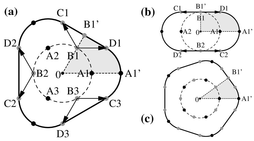
Fig. 8.: (a) Geometrical construction of the deformed billiard ($N=3$), starting form the unit circle billiard. (b) The stadium billiard as an $N=2$ deformed billiard. (c) Deformed billiard for $N=5$. The highlighted regions correspond to “elementary sectors” for which simple GOE level spacing distribution is expected.

Inspired by the billiard stadium problem, we propose a closely related numerical experiment which tests the appearance of the distribution $P^{(N)}(s)$ (D7). For this purpose we determine the energy levels corresponding to a deformation of the circle billiard involving an $N$-fold symmetry axis. Let us consider $N$ equidistant points $A_{i}$, $i=1,...,N$ on the unit circle, with center $O$. $B_{i}$ is the midpoint of the arc of circle $A_{i}A_{i+1}$. We construct then points $C_{i}$ and $D_{i}$ by translating $B_{i}$ with the vectors $\epsilon\cdot\mathchoice{{\hbox{\boldmath$\displaystyle OA_{i+1}$}}}{{\hbox{\boldmath$\textstyle OA_{i+1}$}}}{{\hbox{\boldmath$\scriptstyle OA_{i+1}$}}}{{\hbox{\boldmath$\scriptscriptstyle OA_{i+1}$}}}$ and $\epsilon\cdot\mathchoice{{\hbox{\boldmath$\displaystyle OA_{i}$}}}{{\hbox{\boldmath$\textstyle OA_{i}$}}}{{\hbox{\boldmath$\scriptstyle OA_{i}$}}}{{\hbox{\boldmath$\scriptscriptstyle OA_{i}$}}}$, respectively. The parameter $\epsilon$ controls the degree of the deformation. The deformed billiard is defined by the linear segments $D_{i}C_{i}$ and the arcs of circle $C_{i}D_{i+1}$ with unit radii. The new billiard, for $N=3$ and $\epsilon=1$, is illustrated in Fig. 8a. In the limit $\epsilon\rightarrow 0$ one recovers the original circle billiard. For $N=2$, the new billiard is actually the stadium billiard, as shown in Fig. 8b. For $N>2$, the billiards can be regarded as a generalization of the stadium billiard; this is illustrated for another case, $N=5$, in Fig. 8c.

For a given $N$, the deformed billiard possesses $N$ symmetry planes and, therefore, the corresponding stationary states fall into $2N$ distinct symmetry classes, according to their parity with respect to reflection at these $N$ planes. Proceeding as in the case of the stadium billiard, one can divide the deformed billiard into $2N$ elementary sectors (see the highlighted regions in Fig. 8). The energy levels of a single sector should have an energy spectrum with GOE statistics. This is, indeed, born out of a BEM calculation as shown by the corresponding match with a GOE distribution in Fig. 9a in case of a single $N=5$ sector. A billiard formed by attaching $n$ ($n\leq 2N$) such elementary sectors should exhibit a level spacing distribution given by $P^{(n)}(s)$, while the level spacing distribution corresponding to the full deformed billiard should conform to $P^{(2N)}(s)$. The level spacing distribution of an $N=5$ billiard conforms well to the distribution $P^{(10)}(s)$ as seen in Fig. 9b.

Fig. 9.: Histogram of the energy level spacing distribution $P(s)$ corresponding to $N=5$ for (a) an elementary sector, and (b) full deformed billiards. The level spacing distribution for the elementary sector (full) deformed billiard is well approximated by the GOE $\left[P^{(10)}(s)\right]$ distribution function (solid line). $P(s)$ for the full billiard differs only slightly from the Poisson distribution (dashed line).

In the limit $N\rightarrow\infty$ the deformed billiard becomes a circle of radius $1+\epsilon$ as one can infer readily from the construction presented in Fig. 8. The suggested billiards produce then level spacing distributions which, due to $\lim_{N\rightarrow\infty}P^{(N)}(s)=P_{o}(s)$, conform to a Poisson distribution. This is to be expected, of course, since this distribution governs the spectrum of a circle billiard. One can recognize in Fig. 9b that already in the case $N\,=\,5$ the level spacing distribution resembles the Poisson distribution.

Many further billiards can be constructed in a similar way. For the case of classical systems, a family of billiards which exhibit chaotic as well as mixed chaotic and regular motion have been studied in Ref. [35]. The application of the BEM to determine level statistics as well as wave functions for the mixed system might reveal some surprising behavior.

IV Other Examples

In this section we wish to present two other examples in which the BIM can be applied. Both examples exhibit the features mentioned at the end of Sec. II: (i) the corresponding Green’s function is known analytically; (ii) the boundary condition at $\Gamma$ assumes a simple form. Due to lack of space we shall only outline the BIM treatment of these examples. The interested reader is encouraged to work out further details, including the statistical analysis of the obtained data, in analogy to the quantum billiard case presented in the previous section.

A Finite Potential Well

As a first example let us consider a particle trapped inside a two-dimensional potential well defined by a finite potential increase at the boundary, described by the potential

$$V(\mathchoice{{\hbox{\boldmath$\displaystyle r$}}}{{\hbox{\boldmath$\textstyle r$}}}{{\hbox{\boldmath$\scriptstyle r$}}}{{\hbox{\boldmath$\scriptscriptstyle r$}}})\;=\;\left\{\begin{array}[]{llll}0&,&\text{for}&\mathchoice{{\hbox{\boldmath$\displaystyle r$}}}{{\hbox{\boldmath$\textstyle r$}}}{{\hbox{\boldmath$\scriptstyle r$}}}{{\hbox{\boldmath$\scriptscriptstyle r$}}}\in{\cal D}_{i}\\ V_{o}&,&\text{for}&\mathchoice{{\hbox{\boldmath$\displaystyle r$}}}{{\hbox{\boldmath$\textstyle r$}}}{{\hbox{\boldmath$\scriptstyle r$}}}{{\hbox{\boldmath$\scriptscriptstyle r$}}}\in{\cal D}_{o}\;.\end{array}\right.$$ (55)

Here ${\cal D}_{i/o}$ represents the inner/outer region determined by a closed boundary $\Gamma$ of arbitrary shape. The depth of the potential well is $V_{o}\,(>0)$. The energy spectrum for this system has a discrete part for $E_{n}<V_{o}$, and a continuous part for $E>V_{o}$. The quantum billiard studied in the previous section can be regarded as a limiting case of the present case corresponding to $V_{o}\rightarrow\infty$.

For the purpose of calculating the discrete energy eigenvalues of the system one applies the BIM presented in Sec. II for both inner (${\cal D}_{i}$) and outer (${\cal D}_{o}$) regions. As a result one obtains a set of two coupled BIE’s; the two unknown functions are the wave function $\psi_{n}$ and its outward (with respect to the inner region ${\cal D}_{i}$) normal derivative $\partial_{\nu}\psi_{n}$ along $\Gamma$.

For ${\cal D}\equiv{\cal D}_{i}$, in analogy to Eq.(15), the corresponding BIE reads

$$\psi^{(i)}_{n}(\mathchoice{{\hbox{\boldmath$\displaystyle r^{\prime}$}}}{{\hbox{\boldmath$\textstyle r^{\prime}$}}}{{\hbox{\boldmath$\scriptstyle r^{\prime}$}}}{{\hbox{\boldmath$\scriptscriptstyle r^{\prime}$}}})\;=\;\frac{\hbar^{2}}{m}{\cal P}\oint_{\Gamma}\!ds(\mathchoice{{\hbox{\boldmath$\displaystyle r$}}}{{\hbox{\boldmath$\textstyle r$}}}{{\hbox{\boldmath$\scriptstyle r$}}}{{\hbox{\boldmath$\scriptscriptstyle r$}}})\left[\psi^{(i)}_{n}(\mathchoice{{\hbox{\boldmath$\displaystyle r$}}}{{\hbox{\boldmath$\textstyle r$}}}{{\hbox{\boldmath$\scriptstyle r$}}}{{\hbox{\boldmath$\scriptscriptstyle r$}}})\partial_{\nu}G^{(i)}\left(\mathchoice{{\hbox{\boldmath$\displaystyle r$}}}{{\hbox{\boldmath$\textstyle r$}}}{{\hbox{\boldmath$\scriptstyle r$}}}{{\hbox{\boldmath$\scriptscriptstyle r$}}},\mathchoice{{\hbox{\boldmath$\displaystyle r^{\prime}$}}}{{\hbox{\boldmath$\textstyle r^{\prime}$}}}{{\hbox{\boldmath$\scriptstyle r^{\prime}$}}}{{\hbox{\boldmath$\scriptscriptstyle r^{\prime}$}}};E_{n}\right)-G^{(i)}\left(\mathchoice{{\hbox{\boldmath$\displaystyle r$}}}{{\hbox{\boldmath$\textstyle r$}}}{{\hbox{\boldmath$\scriptstyle r$}}}{{\hbox{\boldmath$\scriptscriptstyle r$}}},\mathchoice{{\hbox{\boldmath$\displaystyle r^{\prime}$}}}{{\hbox{\boldmath$\textstyle r^{\prime}$}}}{{\hbox{\boldmath$\scriptstyle r^{\prime}$}}}{{\hbox{\boldmath$\scriptscriptstyle r^{\prime}$}}};E_{n}\right)\partial_{\nu}\psi^{(i)}_{n}(\mathchoice{{\hbox{\boldmath$\displaystyle r$}}}{{\hbox{\boldmath$\textstyle r$}}}{{\hbox{\boldmath$\scriptstyle r$}}}{{\hbox{\boldmath$\scriptscriptstyle r$}}})\right]\;,$$ (57)

with the Green’s function

$$G^{(i)}\left(\mathchoice{{\hbox{\boldmath$\displaystyle r$}}}{{\hbox{\boldmath$\textstyle r$}}}{{\hbox{\boldmath$\scriptstyle r$}}}{{\hbox{\boldmath$\scriptscriptstyle r$}}},\mathchoice{{\hbox{\boldmath$\displaystyle r^{\prime}$}}}{{\hbox{\boldmath$\textstyle r^{\prime}$}}}{{\hbox{\boldmath$\scriptstyle r^{\prime}$}}}{{\hbox{\boldmath$\scriptscriptstyle r^{\prime}$}}};E_{n}\right)\;=\;-\frac{im}{2\hbar^{2}}H_{0}^{(1)}\left(k_{n}\left|\mathchoice{{\hbox{\boldmath$\displaystyle r$}}}{{\hbox{\boldmath$\textstyle r$}}}{{\hbox{\boldmath$\scriptstyle r$}}}{{\hbox{\boldmath$\scriptscriptstyle r$}}}-\mathchoice{{\hbox{\boldmath$\displaystyle r^{\prime}$}}}{{\hbox{\boldmath$\textstyle r^{\prime}$}}}{{\hbox{\boldmath$\scriptstyle r^{\prime}$}}}{{\hbox{\boldmath$\scriptscriptstyle r^{\prime}$}}}\right|\right)\;,\qquad k_{n}\;=\;\sqrt{2mE_{n}}/\hbar\;.$$ (58)

The “exterior problem” ${\cal D}\equiv{\cal D}_{o}$ requires a more careful treatment due to the fact that ${\cal D}_{o}$ is unbounded. One can circumvent this difficulty by considering instead a finite region ${\cal D}_{\rho}$ delimited by $\Gamma$ inside and by a circle ${\cal C}_{\rho}$ with a very large radius $\rho$ outside, the center of the later located somewhere inside the region ${\cal D}_{i}$; evidently, $\lim_{\rho\rightarrow\infty}{\cal D}_{\rho}={\cal D}_{o}$. Thus, when we apply Green’s formula to obtain the BIE an extra term results in (15) due to the circle ${\cal C}_{\rho}$. However, this extra term vanishes in the limit $\rho\rightarrow\infty$ because for bound states (the only ones we are interested in) both the wave function $\psi^{(o)}_{n}$ and its gradient $\nabla\psi^{(o)}_{n}$ vanish exponentially at infinity. Hence, the corresponding BIE becomes

$$\psi^{(o)}_{n}(\mathchoice{{\hbox{\boldmath$\displaystyle r^{\prime}$}}}{{\hbox{\boldmath$\textstyle r^{\prime}$}}}{{\hbox{\boldmath$\scriptstyle r^{\prime}$}}}{{\hbox{\boldmath$\scriptscriptstyle r^{\prime}$}}})\;=\;-\frac{\hbar^{2}}{m}\,{\cal P}\!\oint_{\Gamma}\!ds(\mathchoice{{\hbox{\boldmath$\displaystyle r$}}}{{\hbox{\boldmath$\textstyle r$}}}{{\hbox{\boldmath$\scriptstyle r$}}}{{\hbox{\boldmath$\scriptscriptstyle r$}}})\left[\psi^{(o)}_{n}(\mathchoice{{\hbox{\boldmath$\displaystyle r$}}}{{\hbox{\boldmath$\textstyle r$}}}{{\hbox{\boldmath$\scriptstyle r$}}}{{\hbox{\boldmath$\scriptscriptstyle r$}}})\partial_{\nu}G^{(o)}\left(\mathchoice{{\hbox{\boldmath$\displaystyle r$}}}{{\hbox{\boldmath$\textstyle r$}}}{{\hbox{\boldmath$\scriptstyle r$}}}{{\hbox{\boldmath$\scriptscriptstyle r$}}},\mathchoice{{\hbox{\boldmath$\displaystyle r^{\prime}$}}}{{\hbox{\boldmath$\textstyle r^{\prime}$}}}{{\hbox{\boldmath$\scriptstyle r^{\prime}$}}}{{\hbox{\boldmath$\scriptscriptstyle r^{\prime}$}}};E_{n}\right)-G^{(o)}\left(\mathchoice{{\hbox{\boldmath$\displaystyle r$}}}{{\hbox{\boldmath$\textstyle r$}}}{{\hbox{\boldmath$\scriptstyle r$}}}{{\hbox{\boldmath$\scriptscriptstyle r$}}},\mathchoice{{\hbox{\boldmath$\displaystyle r^{\prime}$}}}{{\hbox{\boldmath$\textstyle r^{\prime}$}}}{{\hbox{\boldmath$\scriptstyle r^{\prime}$}}}{{\hbox{\boldmath$\scriptscriptstyle r^{\prime}$}}};E_{n}\right)\partial_{\nu}\psi^{(o)}_{n}(\mathchoice{{\hbox{\boldmath$\displaystyle r$}}}{{\hbox{\boldmath$\textstyle r$}}}{{\hbox{\boldmath$\scriptstyle r$}}}{{\hbox{\boldmath$\scriptscriptstyle r$}}})\right]\;,$$ (60)

with the Green’s function (which is finite for $|\mathchoice{{\hbox{\boldmath$\displaystyle r$}}}{{\hbox{\boldmath$\textstyle r$}}}{{\hbox{\boldmath$\scriptstyle r$}}}{{\hbox{\boldmath$\scriptscriptstyle r$}}}-\mathchoice{{\hbox{\boldmath$\displaystyle r^{\prime}$}}}{{\hbox{\boldmath$\textstyle r^{\prime}$}}}{{\hbox{\boldmath$\scriptstyle r^{\prime}$}}}{{\hbox{\boldmath$\scriptscriptstyle r^{\prime}$}}}|\rightarrow\infty$)

$$G^{(o)}\left(\mathchoice{{\hbox{\boldmath$\displaystyle r$}}}{{\hbox{\boldmath$\textstyle r$}}}{{\hbox{\boldmath$\scriptstyle r$}}}{{\hbox{\boldmath$\scriptscriptstyle r$}}},\mathchoice{{\hbox{\boldmath$\displaystyle r^{\prime}$}}}{{\hbox{\boldmath$\textstyle r^{\prime}$}}}{{\hbox{\boldmath$\scriptstyle r^{\prime}$}}}{{\hbox{\boldmath$\scriptscriptstyle r^{\prime}$}}};E_{n}\right)\;=\;-\frac{i\,m}{2\hbar^{2}}H_{0}^{(1)}\left(iq_{n}\left|\mathchoice{{\hbox{\boldmath$\displaystyle r$}}}{{\hbox{\boldmath$\textstyle r$}}}{{\hbox{\boldmath$\scriptstyle r$}}}{{\hbox{\boldmath$\scriptscriptstyle r$}}}-\mathchoice{{\hbox{\boldmath$\displaystyle r^{\prime}$}}}{{\hbox{\boldmath$\textstyle r^{\prime}$}}}{{\hbox{\boldmath$\scriptstyle r^{\prime}$}}}{{\hbox{\boldmath$\scriptscriptstyle r^{\prime}$}}}\right|\right)\;=\;-\frac{1}{\pi}K_{0}\left(q_{n}\left|\mathchoice{{\hbox{\boldmath$\displaystyle r$}}}{{\hbox{\boldmath$\textstyle r$}}}{{\hbox{\boldmath$\scriptstyle r$}}}{{\hbox{\boldmath$\scriptscriptstyle r$}}}-\mathchoice{{\hbox{\boldmath$\displaystyle r^{\prime}$}}}{{\hbox{\boldmath$\textstyle r^{\prime}$}}}{{\hbox{\boldmath$\scriptstyle r^{\prime}$}}}{{\hbox{\boldmath$\scriptscriptstyle r^{\prime}$}}}\right|\right)\;,$$ (61)

$\displaystyle q_{n}\;=\;\sqrt{2m\left(V_{o}-E_{n}\right)}/\hbar\;.$Here $K_{0}(z)$ is a Bessel function of imaginary argument[23] (see also Appendix A). Note the minus sign on the RHS of Eq.(60) which accounts for the opposite orientation of the exterior normal unit vectors corresponding to ${\cal D}_{i}$ and ${\cal D}_{o}$.

Since the wave function and its normal derivative must be continuous across $\Gamma$, i.e.,

$$\psi^{(i)}_{n}(\mathchoice{{\hbox{\boldmath$\displaystyle r$}}}{{\hbox{\boldmath$\textstyle r$}}}{{\hbox{\boldmath$\scriptstyle r$}}}{{\hbox{\boldmath$\scriptscriptstyle r$}}})\;=\;\psi^{(o)}_{n}(\mathchoice{{\hbox{\boldmath$\displaystyle r$}}}{{\hbox{\boldmath$\textstyle r$}}}{{\hbox{\boldmath$\scriptstyle r$}}}{{\hbox{\boldmath$\scriptscriptstyle r$}}})\;\equiv\;\psi_{n}(\mathchoice{{\hbox{\boldmath$\displaystyle r$}}}{{\hbox{\boldmath$\textstyle r$}}}{{\hbox{\boldmath$\scriptstyle r$}}}{{\hbox{\boldmath$\scriptscriptstyle r$}}})\;,$$ (63)

$$\partial_{\nu}\psi^{(i)}_{n}(\mathchoice{{\hbox{\boldmath$\displaystyle r$}}}{{\hbox{\boldmath$\textstyle r$}}}{{\hbox{\boldmath$\scriptstyle r$}}}{{\hbox{\boldmath$\scriptscriptstyle r$}}})\;=\;\partial_{\nu}\psi^{(o)}_{n}(\mathchoice{{\hbox{\boldmath$\displaystyle r$}}}{{\hbox{\boldmath$\textstyle r$}}}{{\hbox{\boldmath$\scriptstyle r$}}}{{\hbox{\boldmath$\scriptscriptstyle r$}}})\;\equiv\;\partial_{\nu}\psi_{n}(\mathchoice{{\hbox{\boldmath$\displaystyle r$}}}{{\hbox{\boldmath$\textstyle r$}}}{{\hbox{\boldmath$\scriptstyle r$}}}{{\hbox{\boldmath$\scriptscriptstyle r$}}})\;,$$ (64)

Eqs.(IV A-IV A) form a set of coupled BIE’s with respect to the unknown functions $\psi_{n}$ and $\partial_{\nu}\psi_{n}$.

The numerical calculation of the energy levels of a particle in a finite two-dimensional potential well proceeds similarly as in the case of a quantum billiard. The steps to be filled in are the same as those discussed in Secs. III A,III B. Note, however, that due to the simultaneous presence of both $\psi_{n}$ and $\partial_{\nu}\psi_{n}$ in the BIE’s, only Method II can be applied in this particular case.

B Quantum Billiard in a Magnetic Field

As a second example, let us consider a charged particle confined to a two-dimensional billiard with $V_{o}\rightarrow\infty$ [cf. Eq.(55)], in the presence of a uniform magnetic field $\textstyle B$ perpendicular to the plane of motion. The Hamiltonian for such quantum billiard in a magnetic field is given by [cf. Eq.(6)]

$$\hat{H}\;=\;\frac{1}{2m}\left(\mathchoice{{\hbox{\boldmath$\displaystyle p$}}}{{\hbox{\boldmath$\textstyle p$}}}{{\hbox{\boldmath$\scriptstyle p$}}}{{\hbox{\boldmath$\scriptscriptstyle p$}}}-q\mathchoice{{\hbox{\boldmath$\displaystyle A$}}}{{\hbox{\boldmath$\textstyle A$}}}{{\hbox{\boldmath$\scriptstyle A$}}}{{\hbox{\boldmath$\scriptscriptstyle A$}}}\right)^{2}+V(\mathchoice{{\hbox{\boldmath$\displaystyle r$}}}{{\hbox{\boldmath$\textstyle r$}}}{{\hbox{\boldmath$\scriptstyle r$}}}{{\hbox{\boldmath$\scriptscriptstyle r$}}})\;,$$ (65)

where $\mathchoice{{\hbox{\boldmath$\displaystyle p$}}}{{\hbox{\boldmath$\textstyle p$}}}{{\hbox{\boldmath$\scriptstyle p$}}}{{\hbox{\boldmath$\scriptscriptstyle p$}}}=-i\hbar\nabla$ is the momentum operator, $q$ is the electric charge of the particle, $\mathchoice{{\hbox{\boldmath$\displaystyle A$}}}{{\hbox{\boldmath$\textstyle A$}}}{{\hbox{\boldmath$\scriptstyle A$}}}{{\hbox{\boldmath$\scriptscriptstyle A$}}}(\mathchoice{{\hbox{\boldmath$\displaystyle r$}}}{{\hbox{\boldmath$\textstyle r$}}}{{\hbox{\boldmath$\scriptstyle r$}}}{{\hbox{\boldmath$\scriptscriptstyle r$}}})$ is the vector potential ($\mathchoice{{\hbox{\boldmath$\displaystyle B$}}}{{\hbox{\boldmath$\textstyle B$}}}{{\hbox{\boldmath$\scriptstyle B$}}}{{\hbox{\boldmath$\scriptscriptstyle B$}}}=\nabla\times\mathchoice{{\hbox{\boldmath$\displaystyle A$}}}{{\hbox{\boldmath$\textstyle A$}}}{{\hbox{\boldmath$\scriptstyle A$}}}{{\hbox{\boldmath$\scriptscriptstyle A$}}}$) and $V(\mathchoice{{\hbox{\boldmath$\displaystyle r$}}}{{\hbox{\boldmath$\textstyle r$}}}{{\hbox{\boldmath$\scriptstyle r$}}}{{\hbox{\boldmath$\scriptscriptstyle r$}}})$ is the scalar potential as given by Eq.(55). The energy spectrum of the system can be determined by solving the Schrödinger equation (1) subject to the Dirichlet boundary condition (18). To derive the corresponding BIE we rewrite the Hamiltonian (65), recalling that for a static magnetic field $\nabla\cdot\mathchoice{{\hbox{\boldmath$\displaystyle A$}}}{{\hbox{\boldmath$\textstyle A$}}}{{\hbox{\boldmath$\scriptstyle A$}}}{{\hbox{\boldmath$\scriptscriptstyle A$}}}=0$,

$$\hat{H}\;=\;-\frac{\hbar^{2}}{2m}\nabla^{2}+\frac{q^{2}A^{2}}{2m}-i\,\frac{q\hbar}{m}\mathchoice{{\hbox{\boldmath$\displaystyle A$}}}{{\hbox{\boldmath$\textstyle A$}}}{{\hbox{\boldmath$\scriptstyle A$}}}{{\hbox{\boldmath$\scriptscriptstyle A$}}}\cdot\nabla\;,$$ (66)

and define the Green’s function $G(\mathchoice{{\hbox{\boldmath$\displaystyle r$}}}{{\hbox{\boldmath$\textstyle r$}}}{{\hbox{\boldmath$\scriptstyle r$}}}{{\hbox{\boldmath$\scriptscriptstyle r$}}},\mathchoice{{\hbox{\boldmath$\displaystyle r^{\prime}$}}}{{\hbox{\boldmath$\textstyle r^{\prime}$}}}{{\hbox{\boldmath$\scriptstyle r^{\prime}$}}}{{\hbox{\boldmath$\scriptscriptstyle r^{\prime}$}}};E)$ as the solution of

$$\left[E-\hat{H}^{*}(\mathchoice{{\hbox{\boldmath$\displaystyle r$}}}{{\hbox{\boldmath$\textstyle r$}}}{{\hbox{\boldmath$\scriptstyle r$}}}{{\hbox{\boldmath$\scriptscriptstyle r$}}})\right]G\left(\mathchoice{{\hbox{\boldmath$\displaystyle r$}}}{{\hbox{\boldmath$\textstyle r$}}}{{\hbox{\boldmath$\scriptstyle r$}}}{{\hbox{\boldmath$\scriptscriptstyle r$}}},\mathchoice{{\hbox{\boldmath$\displaystyle r^{\prime}$}}}{{\hbox{\boldmath$\textstyle r^{\prime}$}}}{{\hbox{\boldmath$\scriptstyle r^{\prime}$}}}{{\hbox{\boldmath$\scriptscriptstyle r^{\prime}$}}};E\right)\;=\;\delta\left(\mathchoice{{\hbox{\boldmath$\displaystyle r$}}}{{\hbox{\boldmath$\textstyle r$}}}{{\hbox{\boldmath$\scriptstyle r$}}}{{\hbox{\boldmath$\scriptscriptstyle r$}}}-\mathchoice{{\hbox{\boldmath$\displaystyle r^{\prime}$}}}{{\hbox{\boldmath$\textstyle r^{\prime}$}}}{{\hbox{\boldmath$\scriptstyle r^{\prime}$}}}{{\hbox{\boldmath$\scriptscriptstyle r^{\prime}$}}}\right)\;,$$ (67)

where $\hat{H}^{*}$ is the complex conjugate of the Hamiltonian (66). Note that $\hat{H}^{*}\neq\hat{H}$, which implies that the magnetic field breaks time reversal symmetry[30].

Using the same strategy as in Sec. II, one can derive the following BIE

$$\psi_{n}(\mathchoice{{\hbox{\boldmath$\displaystyle r^{\prime}$}}}{{\hbox{\boldmath$\textstyle r^{\prime}$}}}{{\hbox{\boldmath$\scriptstyle r^{\prime}$}}}{{\hbox{\boldmath$\scriptscriptstyle r^{\prime}$}}}) \;=\; \frac{\hbar^{2}}{m}{\cal P}\oint_{\Gamma}\!ds(\mathchoice{{\hbox{\boldmath$\displaystyle r$}}}{{\hbox{\boldmath$\textstyle r$}}}{{\hbox{\boldmath$\scriptstyle r$}}}{{\hbox{\boldmath$\scriptscriptstyle r$}}})\left[\psi_{n}(\mathchoice{{\hbox{\boldmath$\displaystyle r$}}}{{\hbox{\boldmath$\textstyle r$}}}{{\hbox{\boldmath$\scriptstyle r$}}}{{\hbox{\boldmath$\scriptscriptstyle r$}}})\partial_{\nu}G\left(\mathchoice{{\hbox{\boldmath$\displaystyle r$}}}{{\hbox{\boldmath$\textstyle r$}}}{{\hbox{\boldmath$\scriptstyle r$}}}{{\hbox{\boldmath$\scriptscriptstyle r$}}},\mathchoice{{\hbox{\boldmath$\displaystyle r^{\prime}$}}}{{\hbox{\boldmath$\textstyle r^{\prime}$}}}{{\hbox{\boldmath$\scriptstyle r^{\prime}$}}}{{\hbox{\boldmath$\scriptscriptstyle r^{\prime}$}}};E_{n}\right)-G\left(\mathchoice{{\hbox{\boldmath$\displaystyle r$}}}{{\hbox{\boldmath$\textstyle r$}}}{{\hbox{\boldmath$\scriptstyle r$}}}{{\hbox{\boldmath$\scriptscriptstyle r$}}},\mathchoice{{\hbox{\boldmath$\displaystyle r^{\prime}$}}}{{\hbox{\boldmath$\textstyle r^{\prime}$}}}{{\hbox{\boldmath$\scriptstyle r^{\prime}$}}}{{\hbox{\boldmath$\scriptscriptstyle r^{\prime}$}}};E_{n}\right)\partial_{\nu}\psi_{n}\left(\mathchoice{{\hbox{\boldmath$\displaystyle r$}}}{{\hbox{\boldmath$\textstyle r$}}}{{\hbox{\boldmath$\scriptstyle r$}}}{{\hbox{\boldmath$\scriptscriptstyle r$}}}\right)\right]$$ (68)

$$\;+\; i\,\frac{2q\hbar}{m}\oint_{\Gamma}\!ds(\mathchoice{{\hbox{\boldmath$\displaystyle r$}}}{{\hbox{\boldmath$\textstyle r$}}}{{\hbox{\boldmath$\scriptstyle r$}}}{{\hbox{\boldmath$\scriptscriptstyle r$}}})A_{\nu}(\mathchoice{{\hbox{\boldmath$\displaystyle r$}}}{{\hbox{\boldmath$\textstyle r$}}}{{\hbox{\boldmath$\scriptstyle r$}}}{{\hbox{\boldmath$\scriptscriptstyle r$}}})G\left(\mathchoice{{\hbox{\boldmath$\displaystyle r$}}}{{\hbox{\boldmath$\textstyle r$}}}{{\hbox{\boldmath$\scriptstyle r$}}}{{\hbox{\boldmath$\scriptscriptstyle r$}}},\mathchoice{{\hbox{\boldmath$\displaystyle r^{\prime}$}}}{{\hbox{\boldmath$\textstyle r^{\prime}$}}}{{\hbox{\boldmath$\scriptstyle r^{\prime}$}}}{{\hbox{\boldmath$\scriptscriptstyle r^{\prime}$}}};E_{n}\right)\psi_{n}(\mathchoice{{\hbox{\boldmath$\displaystyle r$}}}{{\hbox{\boldmath$\textstyle r$}}}{{\hbox{\boldmath$\scriptstyle r$}}}{{\hbox{\boldmath$\scriptscriptstyle r$}}})\;,$$ (69)

where $A_{\nu}\equiv\mathchoice{{\hbox{\boldmath$\displaystyle\nu$}}}{{\hbox{\boldmath$\textstyle\nu$}}}{{\hbox{\boldmath$\scriptstyle\nu$}}}{{\hbox{\boldmath$\scriptscriptstyle\nu$}}}\cdot\mathchoice{{\hbox{\boldmath$\displaystyle A$}}}{{\hbox{\boldmath$\textstyle A$}}}{{\hbox{\boldmath$\scriptstyle A$}}}{{\hbox{\boldmath$\scriptscriptstyle A$}}}$. Since the wave function $\psi_{n}$ vanishes along the boundary of the billiard $\Gamma$ [cf. Eq.(18)] the last term in Eq.(68) can be dropped. As a result, we obtain formally the same BIE as in the field-free case, namely Eq.(19), or equivalently Eq.(39). Hence, the energy levels of a quantum billiard in a magnetic field can be determined as described in Sec. III. The only difference is that, instead of the free particle Green’s function, the Green’s function of a charged particle in magnetic field needs to be used[36]. Here we assume a vector potential corresponding to the symmetric gauge (i.e., $\mathchoice{{\hbox{\boldmath$\displaystyle A$}}}{{\hbox{\boldmath$\textstyle A$}}}{{\hbox{\boldmath$\scriptstyle A$}}}{{\hbox{\boldmath$\scriptscriptstyle A$}}}=\mathchoice{{\hbox{\boldmath$\displaystyle B$}}}{{\hbox{\boldmath$\textstyle B$}}}{{\hbox{\boldmath$\scriptstyle B$}}}{{\hbox{\boldmath$\scriptscriptstyle B$}}}\times\mathchoice{{\hbox{\boldmath$\displaystyle r$}}}{{\hbox{\boldmath$\textstyle r$}}}{{\hbox{\boldmath$\scriptstyle r$}}}{{\hbox{\boldmath$\scriptscriptstyle r$}}}/2$)

$$G\left(\mathchoice{{\hbox{\boldmath$\displaystyle r$}}}{{\hbox{\boldmath$\textstyle r$}}}{{\hbox{\boldmath$\scriptstyle r$}}}{{\hbox{\boldmath$\scriptscriptstyle r$}}},\mathchoice{{\hbox{\boldmath$\displaystyle r^{\prime}$}}}{{\hbox{\boldmath$\textstyle r^{\prime}$}}}{{\hbox{\boldmath$\scriptstyle r^{\prime}$}}}{{\hbox{\boldmath$\scriptscriptstyle r^{\prime}$}}};E_{n}\right)\;=\;e^{i\left(x^{\prime}y-y^{\prime}x\right)/2\ell}\left(-\frac{m}{2\pi\hbar^{2}}\right)\Gamma\left(\frac{1}{2}-\epsilon\right)e^{-z/2}\,U\!\left(\frac{1}{2}-\epsilon,1,z\right)\;,$$ (70)

$\ell=\sqrt{\hbar/m\omega}$ is the so-called magnetic length, $\omega=qB/m$ is the cyclotron frequency, $\varepsilon=E/\hbar\omega$, $z=(\mathchoice{{\hbox{\boldmath$\displaystyle r$}}}{{\hbox{\boldmath$\textstyle r$}}}{{\hbox{\boldmath$\scriptstyle r$}}}{{\hbox{\boldmath$\scriptscriptstyle r$}}}-\mathchoice{{\hbox{\boldmath$\displaystyle r^{\prime}$}}}{{\hbox{\boldmath$\textstyle r^{\prime}$}}}{{\hbox{\boldmath$\scriptstyle r^{\prime}$}}}{{\hbox{\boldmath$\scriptscriptstyle r^{\prime}$}}})^{2}/2\ell^{2}$, $\Gamma(x)$ is the Gamma function[23] and $U(a,b,x)$ is the logarithmic confluent hypergeometric function[23]. The derivation of Eq.(70) is beyond the scope of this article; the reader is referred to Ref. [36].

The above Green’s function can be evaluated numerically by employing the double precision SLATEC subroutines[24] DGAMMA, for the function $\Gamma(x)$, and DCHU, for $U(a,b,x)$. Since the evaluation of the Green’s function and its normal derivative (which can be expressed analytically) is very time consuming in the presence of a magnetic field, it is recommended to apply Method III for determining the energy spectrum of the system.

V Conclusion

In this article we have attempted to provide a self-contained, tutorial like introduction to the Boundary Integral Method for calculating single particle energy spectra in two-dimensional nano-devices. The BIM is suitable whenever (i) a Green’s function $G$ is available analytically and (ii) the boundary condition at the boundary of the device is fairly simple. The method applies to arbitrary shapes of the boundary.

As we have shown, the BIM can be successfully applied to calculate the energy spectrum of quantum billiards, allowing one to investigate the quantum signatures of chaos in these systems. The numerical accuracy of the BIM strongly depends on the degree of discretization of the billiard boundary. Unfortunately, by increasing the number of discretization points along the billiard boundary, the needed computational resources seem to increase more rapidly than the accuracy of the calculated energy levels. Since the number of the needed discretization points along the billiard boundary scales linearly with the cutoff wave vector $K_{c}$ [see Eq.(37)], one can conclude that, in fact, the BIM allows one to calculate the lowest few hundred energy levels of any quantum billiard. The determination of higher energy levels, in general, becomes computationally too expensive. Needles to say, the other existing numerical methods for solving the Schrödinger equation present similar or even more stringent limitations and altogether they perform worse than the BIM.

In conclusion, we would like to mention a few experimental confirmations of the energy level fluctuations of quantum billiards described in this article. The revived interest in studying billiard spectra, in the context of quantum chaos, has resulted in beautiful microwave experiments[37, 38] designed to test the theoretical predictions, based mainly on random matrix theories. These experiments exploit the analogy between the Schrödinger wave equation of a quantum particle in an infinite two-dimensional potential well and the Helmholtz equation of the electromagnetic field in a resonant cavity. Thus, by microwave measurements in the range of 0-25 GHz frequency in quasi two-dimensional cavities shaped, e.g., in the form of a quarter stadium billiard, up to few thousands eigenfrequencies were measured in Refs. [37, 38], and found in agreement with spectra obtained by employing the BIM. Microwave measurements[39, 40] resulted also in the direct observation of the eigenfunctions in microwave cavities of different shapes; the eigenfunctions were also found to be in agreement with descriptions by means of the BIM. A very recent microwave (“photon”) billiard measurement[41] allowed for the first time the direct experimental study of the energy level statistics in the presence of broken time reversal symmetry; the level spacing distribution was found to conform to a GUE form.

A Free Particle Green’s Function in 2D

In this appendix we derive the expression of the free particle Green’s function $G\left(\mathchoice{{\hbox{\boldmath$\displaystyle r$}}}{{\hbox{\boldmath$\textstyle r$}}}{{\hbox{\boldmath$\scriptstyle r$}}}{{\hbox{\boldmath$\scriptscriptstyle r$}}},\mathchoice{{\hbox{\boldmath$\displaystyle r^{\prime}$}}}{{\hbox{\boldmath$\textstyle r^{\prime}$}}}{{\hbox{\boldmath$\scriptstyle r^{\prime}$}}}{{\hbox{\boldmath$\scriptscriptstyle r^{\prime}$}}};E\right)$ in two spatial dimensions. The corresponding expression in $d$-dimensions can be obtained in a similar fashion.

The free particle Green’s function is defined as the solution of the equation [cf. Eq.(7)]

$\displaystyle\left(E+\frac{\hbar^{2}}{2m}\nabla_{r}^{2}\right)G\left(\mathchoice{{\hbox{\boldmath$\displaystyle r$}}}{{\hbox{\boldmath$\textstyle r$}}}{{\hbox{\boldmath$\scriptstyle r$}}}{{\hbox{\boldmath$\scriptscriptstyle r$}}},\mathchoice{{\hbox{\boldmath$\displaystyle r^{\prime}$}}}{{\hbox{\boldmath$\textstyle r^{\prime}$}}}{{\hbox{\boldmath$\scriptstyle r^{\prime}$}}}{{\hbox{\boldmath$\scriptscriptstyle r^{\prime}$}}};E\right)\;=\;\delta\left(\mathchoice{{\hbox{\boldmath$\displaystyle r$}}}{{\hbox{\boldmath$\textstyle r$}}}{{\hbox{\boldmath$\scriptstyle r$}}}{{\hbox{\boldmath$\scriptscriptstyle r$}}}-\mathchoice{{\hbox{\boldmath$\displaystyle r^{\prime}$}}}{{\hbox{\boldmath$\textstyle r^{\prime}$}}}{{\hbox{\boldmath$\scriptstyle r^{\prime}$}}}{{\hbox{\boldmath$\scriptscriptstyle r^{\prime}$}}}\right)\;,$or

$$\left(\nabla_{r}^{2}+k^{2}\right)G\left(\mathchoice{{\hbox{\boldmath$\displaystyle r$}}}{{\hbox{\boldmath$\textstyle r$}}}{{\hbox{\boldmath$\scriptstyle r$}}}{{\hbox{\boldmath$\scriptscriptstyle r$}}},\mathchoice{{\hbox{\boldmath$\displaystyle r^{\prime}$}}}{{\hbox{\boldmath$\textstyle r^{\prime}$}}}{{\hbox{\boldmath$\scriptstyle r^{\prime}$}}}{{\hbox{\boldmath$\scriptscriptstyle r^{\prime}$}}};k\right)\;=\;\frac{2m}{\hbar^{2}}\delta\left(\mathchoice{{\hbox{\boldmath$\displaystyle r$}}}{{\hbox{\boldmath$\textstyle r$}}}{{\hbox{\boldmath$\scriptstyle r$}}}{{\hbox{\boldmath$\scriptscriptstyle r$}}}-\mathchoice{{\hbox{\boldmath$\displaystyle r^{\prime}$}}}{{\hbox{\boldmath$\textstyle r^{\prime}$}}}{{\hbox{\boldmath$\scriptstyle r^{\prime}$}}}{{\hbox{\boldmath$\scriptscriptstyle r^{\prime}$}}}\right)\;,$$ (A1)

where $k\equiv\sqrt{2E/m\hbar^{2}}$ is the wave vector of the particle of energy $E$, and we have replaced the energy variable in the Green’s function with $k$, i.e., $G(k)\equiv G(E)$. By changing variables $\mathchoice{{\hbox{\boldmath$\displaystyle R$}}}{{\hbox{\boldmath$\textstyle R$}}}{{\hbox{\boldmath$\scriptstyle R$}}}{{\hbox{\boldmath$\scriptscriptstyle R$}}}=\mathchoice{{\hbox{\boldmath$\displaystyle r$}}}{{\hbox{\boldmath$\textstyle r$}}}{{\hbox{\boldmath$\scriptstyle r$}}}{{\hbox{\boldmath$\scriptscriptstyle r$}}}-\mathchoice{{\hbox{\boldmath$\displaystyle r^{\prime}$}}}{{\hbox{\boldmath$\textstyle r^{\prime}$}}}{{\hbox{\boldmath$\scriptstyle r^{\prime}$}}}{{\hbox{\boldmath$\scriptscriptstyle r^{\prime}$}}}$, which is equivalent to moving the origin of the coordinate system to the point $\textstyle r^{\prime}$, the above equation becomes

$$\left(\nabla_{R}^{2}+k^{2}\right)G(\mathchoice{{\hbox{\boldmath$\displaystyle R$}}}{{\hbox{\boldmath$\textstyle R$}}}{{\hbox{\boldmath$\scriptstyle R$}}}{{\hbox{\boldmath$\scriptscriptstyle R$}}};k)\;=\;\frac{2m}{\hbar^{2}}\delta(\mathchoice{{\hbox{\boldmath$\displaystyle R$}}}{{\hbox{\boldmath$\textstyle R$}}}{{\hbox{\boldmath$\scriptstyle R$}}}{{\hbox{\boldmath$\scriptscriptstyle R$}}})\;,$$ (A2)

where $G(\mathchoice{{\hbox{\boldmath$\displaystyle R$}}}{{\hbox{\boldmath$\textstyle R$}}}{{\hbox{\boldmath$\scriptstyle R$}}}{{\hbox{\boldmath$\scriptscriptstyle R$}}};k)\equiv G(\mathchoice{{\hbox{\boldmath$\displaystyle R$}}}{{\hbox{\boldmath$\textstyle R$}}}{{\hbox{\boldmath$\scriptstyle R$}}}{{\hbox{\boldmath$\scriptscriptstyle R$}}},0;k)$. The fact that Eq.(A2) does not contain $\textstyle r^{\prime}$ and depends only on $\textstyle R$ is the consequence of translational symmetry.

One can solve (A2) by of Fourier transform. Inserting the Fourier representations

$$G(\mathchoice{{\hbox{\boldmath$\displaystyle R$}}}{{\hbox{\boldmath$\textstyle R$}}}{{\hbox{\boldmath$\scriptstyle R$}}}{{\hbox{\boldmath$\scriptscriptstyle R$}}};k)\;=\;\int\frac{d^{2}\mathchoice{{\hbox{\boldmath$\displaystyle q$}}}{{\hbox{\boldmath$\textstyle q$}}}{{\hbox{\boldmath$\scriptstyle q$}}}{{\hbox{\boldmath$\scriptscriptstyle q$}}}}{(2\pi)^{2}}\tilde{G}(\mathchoice{{\hbox{\boldmath$\displaystyle q$}}}{{\hbox{\boldmath$\textstyle q$}}}{{\hbox{\boldmath$\scriptstyle q$}}}{{\hbox{\boldmath$\scriptscriptstyle q$}}};k)\exp(i\mathchoice{{\hbox{\boldmath$\displaystyle q$}}}{{\hbox{\boldmath$\textstyle q$}}}{{\hbox{\boldmath$\scriptstyle q$}}}{{\hbox{\boldmath$\scriptscriptstyle q$}}}\mathchoice{{\hbox{\boldmath$\displaystyle R$}}}{{\hbox{\boldmath$\textstyle R$}}}{{\hbox{\boldmath$\scriptstyle R$}}}{{\hbox{\boldmath$\scriptscriptstyle R$}}})\;,$$ (A3)

and

$$\delta(\mathchoice{{\hbox{\boldmath$\displaystyle R$}}}{{\hbox{\boldmath$\textstyle R$}}}{{\hbox{\boldmath$\scriptstyle R$}}}{{\hbox{\boldmath$\scriptscriptstyle R$}}})\;=\;\int\frac{d^{2}\mathchoice{{\hbox{\boldmath$\displaystyle q$}}}{{\hbox{\boldmath$\textstyle q$}}}{{\hbox{\boldmath$\scriptstyle q$}}}{{\hbox{\boldmath$\scriptscriptstyle q$}}}}{(2\pi)^{2}}\exp(i\mathchoice{{\hbox{\boldmath$\displaystyle q$}}}{{\hbox{\boldmath$\textstyle q$}}}{{\hbox{\boldmath$\scriptstyle q$}}}{{\hbox{\boldmath$\scriptscriptstyle q$}}}\mathchoice{{\hbox{\boldmath$\displaystyle R$}}}{{\hbox{\boldmath$\textstyle R$}}}{{\hbox{\boldmath$\scriptstyle R$}}}{{\hbox{\boldmath$\scriptscriptstyle R$}}})$$ (A4)

in Eq.(A2), and identifying the Fourier coefficients on both sides of the resulting equation, one arrives at

$$(-q^{2}+k^{2})\tilde{G}(\mathchoice{{\hbox{\boldmath$\displaystyle q$}}}{{\hbox{\boldmath$\textstyle q$}}}{{\hbox{\boldmath$\scriptstyle q$}}}{{\hbox{\boldmath$\scriptscriptstyle q$}}};k)\;=\;\frac{2m}{\hbar^{2}}\;.$$ (A5)

Inserting $\tilde{G}$ from (A5) into (A3) results in

$$G(\mathchoice{{\hbox{\boldmath$\displaystyle R$}}}{{\hbox{\boldmath$\textstyle R$}}}{{\hbox{\boldmath$\scriptstyle R$}}}{{\hbox{\boldmath$\scriptscriptstyle R$}}};k)\;=\;\frac{2m}{\hbar^{2}}\int\frac{d^{2}\mathchoice{{\hbox{\boldmath$\displaystyle q$}}}{{\hbox{\boldmath$\textstyle q$}}}{{\hbox{\boldmath$\scriptstyle q$}}}{{\hbox{\boldmath$\scriptscriptstyle q$}}}}{(2\pi)^{2}}\frac{\exp(i\mathchoice{{\hbox{\boldmath$\displaystyle q$}}}{{\hbox{\boldmath$\textstyle q$}}}{{\hbox{\boldmath$\scriptstyle q$}}}{{\hbox{\boldmath$\scriptscriptstyle q$}}}\mathchoice{{\hbox{\boldmath$\displaystyle R$}}}{{\hbox{\boldmath$\textstyle R$}}}{{\hbox{\boldmath$\scriptstyle R$}}}{{\hbox{\boldmath$\scriptscriptstyle R$}}})}{k^{2}-q^{2}}\;.$$ (A6)

The two-dimensional integral is evaluated by using polar coordinates $\mathchoice{{\hbox{\boldmath$\displaystyle q$}}}{{\hbox{\boldmath$\textstyle q$}}}{{\hbox{\boldmath$\scriptstyle q$}}}{{\hbox{\boldmath$\scriptscriptstyle q$}}}=(q,\theta)$ as follows

$$G(\mathchoice{{\hbox{\boldmath$\displaystyle R$}}}{{\hbox{\boldmath$\textstyle R$}}}{{\hbox{\boldmath$\scriptstyle R$}}}{{\hbox{\boldmath$\scriptscriptstyle R$}}};k)\;=\;\frac{m}{\pi\hbar^{2}}\int_{0}^{\infty}\frac{q{dq}}{k^{2}-q^{2}}\frac{1}{2\pi}\int_{0}^{2\pi}{d\theta}\exp(iqR\cos\theta)\;.$$ (A7)

The second integral on the right hand side is identified as one of the integral representations of the 0-th order Bessel function $J_{0}(qR)$ [cf. formula 8.4111. in Ref.[26]] and one obtains

$$G(\mathchoice{{\hbox{\boldmath$\displaystyle R$}}}{{\hbox{\boldmath$\textstyle R$}}}{{\hbox{\boldmath$\scriptstyle R$}}}{{\hbox{\boldmath$\scriptscriptstyle R$}}};k)\;=\;-\frac{m}{\pi\hbar^{2}}\int_{0}^{\infty}{dq}\frac{qJ_{0}(qR)}{q^{2}-k^{2}}\;.$$ (A8)

The integral on the RHS of (A8) is ill defined due to the singularity of the integrand at $q=\pm k$. However, the integral can be regularized by adding to $k$ an infinitely small, positive imaginary part, i.e., $k\rightarrow k+i\varepsilon$. In this case $k^{2}\rightarrow(k+i\varepsilon)^{2}=-(\varepsilon-ik)^{2}$, and according to the formula 6.5324 of Ref.[26] the integral in (A8) is equal to $K_{0}((\varepsilon-ik)R)$, where $K_{0}$ is the MacDonald (modified Bessel) function, which is finite as $R\rightarrow\infty$. After taking the limit $\varepsilon\rightarrow 0^{+}$, one obtains then

$$G(\mathchoice{{\hbox{\boldmath$\displaystyle R$}}}{{\hbox{\boldmath$\textstyle R$}}}{{\hbox{\boldmath$\scriptstyle R$}}}{{\hbox{\boldmath$\scriptscriptstyle R$}}};k)\;=\;-\frac{m}{\pi\hbar^{2}}K_{0}(-ikR)\;.$$ (A9)

Note that for $\varepsilon<0$ the above integral would be divergent for $R\rightarrow\infty$. However, as long as we are not concerned with the $R\rightarrow\infty$ behavior of $G(\mathchoice{{\hbox{\boldmath$\displaystyle R$}}}{{\hbox{\boldmath$\textstyle R$}}}{{\hbox{\boldmath$\scriptstyle R$}}}{{\hbox{\boldmath$\scriptscriptstyle R$}}};k)$, the infinitesimal $\varepsilon$ can be chosen either positive or negative. The choice $\varepsilon>0$ is equivalent to the so-called Sommerfeld radiation condition[42].

Finally, by using the identity $K_{0}(z)=(i\pi/2)H_{0}^{(1)}(iz)$ [formula 8.4071 in Ref.[26]], where $z$ is an arbitrary complex number and $H_{0}^{(1)}$ is the 0-th order Hankel function of the first kind, one arrives at the expression of the free particle Green’s function given by (17).

B Evaluation of the singular integrals in the Boundary Integral Equation

In order to calculate the LHS of Eq.(14), consider first the case when the potential energy $V(\mathchoice{{\hbox{\boldmath$\displaystyle r$}}}{{\hbox{\boldmath$\textstyle r$}}}{{\hbox{\boldmath$\scriptstyle r$}}}{{\hbox{\boldmath$\scriptscriptstyle r$}}})$ is zero and, therefore, the relevant Green’s function is given by (17). For $\varepsilon\equiv|\mathchoice{{\hbox{\boldmath$\displaystyle r$}}}{{\hbox{\boldmath$\textstyle r$}}}{{\hbox{\boldmath$\scriptstyle r$}}}{{\hbox{\boldmath$\scriptscriptstyle r$}}}-\mathchoice{{\hbox{\boldmath$\displaystyle r^{\prime}$}}}{{\hbox{\boldmath$\textstyle r^{\prime}$}}}{{\hbox{\boldmath$\scriptstyle r^{\prime}$}}}{{\hbox{\boldmath$\scriptscriptstyle r^{\prime}$}}}|\rightarrow 0$ one can replace the Hankel function in the above equation by its limiting form for small arguments[43]

$$G\left(\mathchoice{{\hbox{\boldmath$\displaystyle r$}}}{{\hbox{\boldmath$\textstyle r$}}}{{\hbox{\boldmath$\scriptstyle r$}}}{{\hbox{\boldmath$\scriptscriptstyle r$}}},\mathchoice{{\hbox{\boldmath$\displaystyle r^{\prime}$}}}{{\hbox{\boldmath$\textstyle r^{\prime}$}}}{{\hbox{\boldmath$\scriptstyle r^{\prime}$}}}{{\hbox{\boldmath$\scriptscriptstyle r^{\prime}$}}};E_{n}\right)\;\sim\;-\frac{m}{\pi\hbar^{2}}\ln(k\varepsilon)\;,\qquad\varepsilon\rightarrow 0\;.$$ (B1)

Next, we parameterize the arc of circle $C_{\varepsilon}$ through the angle $\varphi$ (see Fig.1) formed by the tangent AT₁ to $\Gamma$ at A$\in\Gamma$ (of position vector $\textstyle r^{\prime}$) and the vector $\textstyle\varepsilon$. The angle $\varphi$ assumes values between zero and $\theta(\mathchoice{{\hbox{\boldmath$\displaystyle r^{\prime}$}}}{{\hbox{\boldmath$\textstyle r^{\prime}$}}}{{\hbox{\boldmath$\scriptstyle r^{\prime}$}}}{{\hbox{\boldmath$\scriptscriptstyle r^{\prime}$}}})=\widehat{\text{T}_{1}\text{AT}_{2}}$, i.e., the exterior angle made by the two tangents to $\Gamma$ at A. If the contour $\Gamma$ is smooth then the tangents coincide and $\theta(\mathchoice{{\hbox{\boldmath$\displaystyle r^{\prime}$}}}{{\hbox{\boldmath$\textstyle r^{\prime}$}}}{{\hbox{\boldmath$\scriptstyle r^{\prime}$}}}{{\hbox{\boldmath$\scriptscriptstyle r^{\prime}$}}})=\pi$. The arc element along $C_{\varepsilon}$ is $ds(\mathchoice{{\hbox{\boldmath$\displaystyle r$}}}{{\hbox{\boldmath$\textstyle r$}}}{{\hbox{\boldmath$\scriptstyle r$}}}{{\hbox{\boldmath$\scriptscriptstyle r$}}})=\varepsilon d\varphi$. Since both $\psi_{n}$ and $\partial_{\nu}\psi_{n}$ are finite, in the limit $\varepsilon\rightarrow 0$ the quantities can be replaced in (14) by their values at $\mathchoice{{\hbox{\boldmath$\displaystyle r$}}}{{\hbox{\boldmath$\textstyle r$}}}{{\hbox{\boldmath$\scriptstyle r$}}}{{\hbox{\boldmath$\scriptscriptstyle r$}}}=\mathchoice{{\hbox{\boldmath$\displaystyle r^{\prime}$}}}{{\hbox{\boldmath$\textstyle r^{\prime}$}}}{{\hbox{\boldmath$\scriptstyle r^{\prime}$}}}{{\hbox{\boldmath$\scriptscriptstyle r^{\prime}$}}}$; one obtains then

$$\lim_{\varepsilon\rightarrow 0}\frac{\hbar^{2}}{2m}\int_{C_{\varepsilon}}\!ds(\mathchoice{{\hbox{\boldmath$\displaystyle r$}}}{{\hbox{\boldmath$\textstyle r$}}}{{\hbox{\boldmath$\scriptstyle r$}}}{{\hbox{\boldmath$\scriptscriptstyle r$}}})G\left(\mathchoice{{\hbox{\boldmath$\displaystyle r$}}}{{\hbox{\boldmath$\textstyle r$}}}{{\hbox{\boldmath$\scriptstyle r$}}}{{\hbox{\boldmath$\scriptscriptstyle r$}}},\mathchoice{{\hbox{\boldmath$\displaystyle r^{\prime}$}}}{{\hbox{\boldmath$\textstyle r^{\prime}$}}}{{\hbox{\boldmath$\scriptstyle r^{\prime}$}}}{{\hbox{\boldmath$\scriptscriptstyle r^{\prime}$}}};E_{n}\right)\partial_{\nu}\psi_{n}(\mathchoice{{\hbox{\boldmath$\displaystyle r$}}}{{\hbox{\boldmath$\textstyle r$}}}{{\hbox{\boldmath$\scriptstyle r$}}}{{\hbox{\boldmath$\scriptscriptstyle r$}}})\;=\;-\frac{1}{2\pi}\lim_{\varepsilon\rightarrow 0}\left[\varepsilon\ln(k\varepsilon)\right]\theta(\mathchoice{{\hbox{\boldmath$\displaystyle r^{\prime}$}}}{{\hbox{\boldmath$\textstyle r^{\prime}$}}}{{\hbox{\boldmath$\scriptstyle r^{\prime}$}}}{{\hbox{\boldmath$\scriptscriptstyle r^{\prime}$}}})\partial_{\nu}\psi_{n}(\mathchoice{{\hbox{\boldmath$\displaystyle r^{\prime}$}}}{{\hbox{\boldmath$\textstyle r^{\prime}$}}}{{\hbox{\boldmath$\scriptstyle r^{\prime}$}}}{{\hbox{\boldmath$\scriptscriptstyle r^{\prime}$}}})\;=\;0\;.$$ (B2)

The integral containing $\partial_{\nu}G$ in (14) can be calculated in a similar fashion. According to Eqs.(12) and (17) one can write successively

$$\partial_{\nu}G\left(\mathchoice{{\hbox{\boldmath$\displaystyle r$}}}{{\hbox{\boldmath$\textstyle r$}}}{{\hbox{\boldmath$\scriptstyle r$}}}{{\hbox{\boldmath$\scriptscriptstyle r$}}},\mathchoice{{\hbox{\boldmath$\displaystyle r^{\prime}$}}}{{\hbox{\boldmath$\textstyle r^{\prime}$}}}{{\hbox{\boldmath$\scriptstyle r^{\prime}$}}}{{\hbox{\boldmath$\scriptscriptstyle r^{\prime}$}}};E_{n}\right) \;=\; \mathchoice{{\hbox{\boldmath$\displaystyle\nu$}}}{{\hbox{\boldmath$\textstyle\nu$}}}{{\hbox{\boldmath$\scriptstyle\nu$}}}{{\hbox{\boldmath$\scriptscriptstyle\nu$}}}(\mathchoice{{\hbox{\boldmath$\displaystyle r$}}}{{\hbox{\boldmath$\textstyle r$}}}{{\hbox{\boldmath$\scriptstyle r$}}}{{\hbox{\boldmath$\scriptscriptstyle r$}}})\cdot\nabla_{r}\left[-\frac{im}{2\hbar^{2}}H_{0}^{(1)}\left(k|\mathchoice{{\hbox{\boldmath$\displaystyle r$}}}{{\hbox{\boldmath$\textstyle r$}}}{{\hbox{\boldmath$\scriptstyle r$}}}{{\hbox{\boldmath$\scriptscriptstyle r$}}}-\mathchoice{{\hbox{\boldmath$\displaystyle r^{\prime}$}}}{{\hbox{\boldmath$\textstyle r^{\prime}$}}}{{\hbox{\boldmath$\scriptstyle r^{\prime}$}}}{{\hbox{\boldmath$\scriptscriptstyle r^{\prime}$}}}|\right)\right]$$ (B3)

$$\;=\; \frac{imk}{2\hbar^{2}}\>\left[\mathchoice{{\hbox{\boldmath$\displaystyle\nu$}}}{{\hbox{\boldmath$\textstyle\nu$}}}{{\hbox{\boldmath$\scriptstyle\nu$}}}{{\hbox{\boldmath$\scriptscriptstyle\nu$}}}(\mathchoice{{\hbox{\boldmath$\displaystyle r$}}}{{\hbox{\boldmath$\textstyle r$}}}{{\hbox{\boldmath$\scriptstyle r$}}}{{\hbox{\boldmath$\scriptscriptstyle r$}}})\cdot\frac{\mathchoice{{\hbox{\boldmath$\displaystyle r$}}}{{\hbox{\boldmath$\textstyle r$}}}{{\hbox{\boldmath$\scriptstyle r$}}}{{\hbox{\boldmath$\scriptscriptstyle r$}}}-\mathchoice{{\hbox{\boldmath$\displaystyle r^{\prime}$}}}{{\hbox{\boldmath$\textstyle r^{\prime}$}}}{{\hbox{\boldmath$\scriptstyle r^{\prime}$}}}{{\hbox{\boldmath$\scriptscriptstyle r^{\prime}$}}}}{|\mathchoice{{\hbox{\boldmath$\displaystyle r$}}}{{\hbox{\boldmath$\textstyle r$}}}{{\hbox{\boldmath$\scriptstyle r$}}}{{\hbox{\boldmath$\scriptscriptstyle r$}}}-\mathchoice{{\hbox{\boldmath$\displaystyle r^{\prime}$}}}{{\hbox{\boldmath$\textstyle r^{\prime}$}}}{{\hbox{\boldmath$\scriptstyle r^{\prime}$}}}{{\hbox{\boldmath$\scriptscriptstyle r^{\prime}$}}}|}\right]\>H_{1}^{(1)}\left(k|\mathchoice{{\hbox{\boldmath$\displaystyle r$}}}{{\hbox{\boldmath$\textstyle r$}}}{{\hbox{\boldmath$\scriptstyle r$}}}{{\hbox{\boldmath$\scriptscriptstyle r$}}}-\mathchoice{{\hbox{\boldmath$\displaystyle r^{\prime}$}}}{{\hbox{\boldmath$\textstyle r^{\prime}$}}}{{\hbox{\boldmath$\scriptstyle r^{\prime}$}}}{{\hbox{\boldmath$\scriptscriptstyle r^{\prime}$}}}|\right)\;,$$ (B4)

where we used $dH_{0}^{(1)}(z)/dz=-H_{1}^{(1)}(z)$ [cf. formula 9.1.30 in Ref.[23]]. On the arc of circle $C_{\varepsilon}$ the dot product in (B3) is equal to one (see Fig.1); taking into account the limiting form of $H_{1}^{(1)}$ for small arguments[43], one can write

$$\lim_{\varepsilon\rightarrow 0}\frac{\hbar^{2}}{2m}\int_{C_{\varepsilon}}\!ds(\mathchoice{{\hbox{\boldmath$\displaystyle r$}}}{{\hbox{\boldmath$\textstyle r$}}}{{\hbox{\boldmath$\scriptstyle r$}}}{{\hbox{\boldmath$\scriptscriptstyle r$}}})\psi_{n}(\mathchoice{{\hbox{\boldmath$\displaystyle r$}}}{{\hbox{\boldmath$\textstyle r$}}}{{\hbox{\boldmath$\scriptstyle r$}}}{{\hbox{\boldmath$\scriptscriptstyle r$}}})\partial_{\nu}G\left(\mathchoice{{\hbox{\boldmath$\displaystyle r$}}}{{\hbox{\boldmath$\textstyle r$}}}{{\hbox{\boldmath$\scriptstyle r$}}}{{\hbox{\boldmath$\scriptscriptstyle r$}}},\mathchoice{{\hbox{\boldmath$\displaystyle r^{\prime}$}}}{{\hbox{\boldmath$\textstyle r^{\prime}$}}}{{\hbox{\boldmath$\scriptstyle r^{\prime}$}}}{{\hbox{\boldmath$\scriptscriptstyle r^{\prime}$}}};E_{n}\right) \;=\; \frac{\hbar^{2}}{2m}\psi_{n}(\mathchoice{{\hbox{\boldmath$\displaystyle r^{\prime}$}}}{{\hbox{\boldmath$\textstyle r^{\prime}$}}}{{\hbox{\boldmath$\scriptstyle r^{\prime}$}}}{{\hbox{\boldmath$\scriptscriptstyle r^{\prime}$}}})\lim_{\varepsilon\rightarrow 0}\int_{0}^{\theta(\mathchoice{{\hbox{\boldmath$\displaystyle r^{\prime}$}}}{{\hbox{\boldmath$\textstyle r^{\prime}$}}}{{\hbox{\boldmath$\scriptstyle r^{\prime}$}}}{{\hbox{\boldmath$\scriptscriptstyle r^{\prime}$}}})}\varepsilon d\varphi\left(\frac{imk}{2\hbar^{2}}\right)\left(-\frac{2i}{\pi k\varepsilon}\right)$$ (B5)

$$\;=\; \frac{\theta(\mathchoice{{\hbox{\boldmath$\displaystyle r^{\prime}$}}}{{\hbox{\boldmath$\textstyle r^{\prime}$}}}{{\hbox{\boldmath$\scriptstyle r^{\prime}$}}}{{\hbox{\boldmath$\scriptscriptstyle r^{\prime}$}}})}{2\pi}\psi_{n}(\mathchoice{{\hbox{\boldmath$\displaystyle r^{\prime}$}}}{{\hbox{\boldmath$\textstyle r^{\prime}$}}}{{\hbox{\boldmath$\scriptstyle r^{\prime}$}}}{{\hbox{\boldmath$\scriptscriptstyle r^{\prime}$}}})\;.$$ (B6)

For a smooth boundary $\Gamma$, where $\theta(\mathchoice{{\hbox{\boldmath$\displaystyle r^{\prime}$}}}{{\hbox{\boldmath$\textstyle r^{\prime}$}}}{{\hbox{\boldmath$\scriptstyle r^{\prime}$}}}{{\hbox{\boldmath$\scriptscriptstyle r^{\prime}$}}})=\pi$, Eqs.(B2-B5) provide the result given in (14).

For a finite potential energy $V(\mathchoice{{\hbox{\boldmath$\displaystyle r$}}}{{\hbox{\boldmath$\textstyle r$}}}{{\hbox{\boldmath$\scriptstyle r$}}}{{\hbox{\boldmath$\scriptscriptstyle r$}}})$, in general, there is no simple analytical expression for the Green’s function $G$ and the validity of Eq.(14) is questionable. However, by assuming on physical grounds that $V(\mathchoice{{\hbox{\boldmath$\displaystyle r$}}}{{\hbox{\boldmath$\textstyle r$}}}{{\hbox{\boldmath$\scriptstyle r$}}}{{\hbox{\boldmath$\scriptscriptstyle r$}}})$ is finite for all $\mathchoice{{\hbox{\boldmath$\displaystyle r$}}}{{\hbox{\boldmath$\textstyle r$}}}{{\hbox{\boldmath$\scriptstyle r$}}}{{\hbox{\boldmath$\scriptscriptstyle r$}}}\in{\cal D}$, one can realize that the result (14) holds in this case too. Indeed, when $\varepsilon$ is small the potential energy is almost constant in the vicinity of $\textstyle r^{\prime}$ (point A in Fig.1) and, therefore, one can approximate the Green’s function with the corresponding expression valid for a constant $V\equiv V(\mathchoice{{\hbox{\boldmath$\displaystyle r^{\prime}$}}}{{\hbox{\boldmath$\textstyle r^{\prime}$}}}{{\hbox{\boldmath$\scriptstyle r^{\prime}$}}}{{\hbox{\boldmath$\scriptscriptstyle r^{\prime}$}}})$. The approximation becomes exact in the limit $\varepsilon\rightarrow 0$. But $G$ for a constant potential energy has essentially the same form as for a free particle [Eq.(17)] and, therefore, it has the same type of logarithmic singularity at $\mathchoice{{\hbox{\boldmath$\displaystyle r$}}}{{\hbox{\boldmath$\textstyle r$}}}{{\hbox{\boldmath$\scriptstyle r$}}}{{\hbox{\boldmath$\scriptscriptstyle r$}}}=\mathchoice{{\hbox{\boldmath$\displaystyle r^{\prime}$}}}{{\hbox{\boldmath$\textstyle r^{\prime}$}}}{{\hbox{\boldmath$\scriptstyle r^{\prime}$}}}{{\hbox{\boldmath$\scriptscriptstyle r^{\prime}$}}}$. Since the actual value of the integral (14) is determined solely by the type of this singularity of the Green’s function one may conclude that the result derived in this appendix holds in general.

C Analytical Solution of the Boundary Integral Equation for a Circular Billiard

In this appendix we solve analytically the BIE (22) for a circular billiard of unit radius. For the unit circle ${\cal L}=2\pi$ and, according to Eq.(25), one finds $K_{j}=j$, with $j=0,\pm 1,\ldots$. By using the Fourier representation (24) for $u(s)$, the BIE becomes

$$\sum_{j=-\infty}^{\infty}u_{j}\int_{0}^{2\pi}\!ds\,G\left(s,s^{\prime};k\right)\exp(ijs)\;=\;0\;.$$ (C1)

The expression (A6) of the free particle Green’s function, in the present case, can be written

$$G\left(s,s^{\prime};k\right) \;=\; \frac{2m}{\hbar^{2}}\int\frac{d^{2}\mathchoice{{\hbox{\boldmath$\displaystyle q$}}}{{\hbox{\boldmath$\textstyle q$}}}{{\hbox{\boldmath$\scriptstyle q$}}}{{\hbox{\boldmath$\scriptscriptstyle q$}}}}{(2\pi)^{2}}\frac{\exp\{i\mathchoice{{\hbox{\boldmath$\displaystyle q$}}}{{\hbox{\boldmath$\textstyle q$}}}{{\hbox{\boldmath$\scriptstyle q$}}}{{\hbox{\boldmath$\scriptscriptstyle q$}}}[\mathchoice{{\hbox{\boldmath$\displaystyle r$}}}{{\hbox{\boldmath$\textstyle r$}}}{{\hbox{\boldmath$\scriptstyle r$}}}{{\hbox{\boldmath$\scriptscriptstyle r$}}}(s)-\mathchoice{{\hbox{\boldmath$\displaystyle r$}}}{{\hbox{\boldmath$\textstyle r$}}}{{\hbox{\boldmath$\scriptstyle r$}}}{{\hbox{\boldmath$\scriptscriptstyle r$}}}(s^{\prime})]\}}{k^{2}-q^{2}}$$ (C2)

$$\;=\; \frac{m}{\pi\hbar^{2}}\int_{0}^{\infty}\frac{qdq}{k^{2}-q^{2}}\frac{1}{2\pi}\int_{0}^{2\pi}d\theta\exp[iq\cos(s-\theta)]\exp[-iq\cos(s^{\prime}-\theta)]\;,$$ (C3)

where $q$ and $\theta$ are the polar coordinates of the 2D vector $\textstyle q$. Inserting (C2) in (C1) one obtains (the irrelevant constant factor $2m/\hbar^{2}$ can be dropped)

$$\sum_{j=-\infty}^{\infty}u_{j}\int_{0}^{\infty}\frac{qdq}{k^{2}-q^{2}}\frac{1}{2\pi}\int_{0}^{2\pi}d\theta\exp[-iq\cos(s^{\prime}-\theta)]$$ (C4)

$$\times\frac{1}{2\pi}\int_{0}^{2\pi}ds\exp[iq\cos(s-\theta)]\exp(ijs) \;=\; 0\;.$$ (C5)

By taking into account the integral representation of the integer Bessel function [formula 8.4111. in Ref.[26]], the integral over $s$ in (C4) can be evaluated exactly as follows

$$\frac{1}{2\pi}\int_{0}^{2\pi}ds\exp[iq\cos(s-\theta)]\exp(ijs) \;=\; \left[\frac{1}{2\pi}\int_{0}^{2\pi}ds\exp\{i[q\cos(s-\theta)+j(s-\theta)]\}\right]$$ (C6)

$$\times\exp(ij\theta) \;=\; i^{j}J_{j}(q)\exp(ij\theta)\;.$$ (C7)

Similarly, the integral with respect to $\theta$ in (C4) gives

$$\frac{1}{2\pi}\int_{0}^{2\pi}d\theta\exp[-iq\cos(s^{\prime}-\theta)]\exp(ij\theta)\;=\;(-i)^{j}J_{j}(q)\exp(ijs^{\prime})\;.$$ (C8)

With the last two results, Eq.(C4) becomes

$$\sum_{j=-\infty}^{\infty}u_{j}\exp(ijs^{\prime})\int_{0}^{\infty}dq\frac{q\left[J_{j}(q)\right]^{2}}{k^{2}-q^{2}}\;=\;0\;.$$ (C9)

By employing formulas 6.535, 8.4061 and 8.4071 in Ref.[26], the integral with respect to $q$ can also be calculated exactly as follows

$$\int_{0}^{\infty}dq\frac{q\left[J_{j}(q)\right]^{2}}{k^{2}-q^{2}}\;=\;-\int_{0}^{\infty}dq\frac{q\left[J_{j}(q)\right]^{2}}{q^{2}+(ik)^{2}}\;=\;-I_{j}(-ik)K_{j}(-ik)\;=\;-\frac{\pi}{2}J_{j}(k)H_{j}^{(1)}(k)\;.$$ (C10)

Here $I_{j}$ and $K_{j}$ are imaginary argument Bessel functions.

Finally, the BIE for the circle billiard of unit radius can be written as

$$\sum_{j=-\infty}^{\infty}u_{j}\exp(ijs^{\prime})J_{j}(k)H_{j}^{(1)}(k)\;=\;0\;,$$ (C11)

Since $\exp(ijs)$, $j=0,\pm 1\ldots$, form a complete orthonormal set, the above equation tells us that the expansion coefficients should be all equal to zero. The eigenenergies correspond to those $k$ values for which non trivial $u_{j}$’s exist. Recalling that the Hankel functions have no real roots, one obtains the same eigenenergy equation (31) as in Sec.III A.

By taking the Fourier transform of Eq.(C11) with respect to $s^{\prime}$, one can see that the matrix $A_{ij}(k)$ defined by (28) is indeed diagonal and

$$A_{ij}(k)\;\propto\;J_{j}(k)H_{j}^{(1)}(k)\>\delta_{ij}\;.$$ (C12)

D Superposition of $N$ Independent Spectra with GOE Level Spacing Distribution

In this Appendix we derive the level spacing distribution function $P^{(N)}(s)$ corresponding to the superposition of $N$ independent spectra with GOE level spacing distribution. In general, $P(s)$ can be expressed[30]

$$P(s)\;=\;\frac{\partial^{2}{\cal E}(s)}{\partial\,s^{2}}\;,$$ (D1)

where ${\cal E}(s)$, the so-called gap probability, gives the probability that the energy interval $(E,E+s)$ lacks energy levels.

Let us consider $N$ independent (i.e., uncorrelated) sets of energy levels with GOE level spacing distribution

$$P_{i}(s)\;=\;\frac{\pi}{2}\frac{s}{N^{2}}\,\exp\left[-\frac{\pi}{4}\left(\frac{s}{N}\right)^{2}\right]\;,\qquad i\>=\>1,\ldots,N$$ (D2)

The probability density (D2) is normalized as follows

$$\int_{0}^{\infty}\!ds\,P_{i}(s)\;=\;1\;,\qquad\langle s_{i}\rangle\;\equiv\;\int_{0}^{\infty}\!ds\>s\,P_{i}(s)\;=\;N\;.$$ (D3)

Note that the choice $\langle s_{i}\rangle=N$ for each set of levels leads to a unit mean level spacing $\langle s^{(N)}\rangle$ for the spectrum comprising all $N$ energy spectra.

According to Eqs.(D1)-(D2), the individual gap probabilities can be expressed as

$${\cal E}_{i}(s) \;=\; \frac{1}{N}\int_{s}^{\infty}\!dx\int_{x}^{\infty}\!dy\,P_{i}(y)$$ (D4)

$$\;=\; \frac{2}{\sqrt{\pi}}\int_{\frac{\sqrt{\pi}\,s}{2N}}^{\infty}\!dt\,\exp\left(-t^{2}\right)\;=\;\text{erfc}\left(\frac{\sqrt{\pi}\,s}{2N}\right)\;,$$ (D5)

where erfc$(z)$ is the complementary error function[23]. Since the energy spectra are uncorrelated, the gap probability of the combined spectrum is given by

$${\cal E}^{(N)}(s)\;=\;\prod_{i=1}^{N}{\cal E}_{i}(s)\;=\;\left[\text{erfc}\left(\frac{\sqrt{\pi}}{2}\frac{s}{N}\right)\right]^{N}\;,$$ (D6)

and, according to (D1), the desired level spacing distribution function becomes

$$P^{(N)}(s)\;=\;\frac{\partial^{2}}{\partial\,s^{2}}\left[\text{erfc}\left(\frac{\sqrt{\pi}}{2}\frac{s}{N}\right)\right]^{N}\;.$$ (D7)

Note that the above method of calculating $P(s)$ is rather general and applies also when the independent spectra have arbitrary statistics. For example, one could calculate the level spacing distribution of the superposition of an arbitrary number of spectra, some of them obeying Poisson statistics and the rest GOE statistics. For further details the reader is referred to Refs. [31, 32].

REFERENCES

- [1] For a recent overview of the exciting fields of mesoscopic physics and nanoelectronics see, e.g., F.A. Buot, “Mesoscopic physics and nanoelectronics: nanoscience and nanotechnology”, Phys. Rep. 234, 73-174 (1993).
- [2] M. Tinkham, “Coulomb blockade and an electron in a mesoscopic box”, Am. J. Phys 64, 343–347 (1996).
- [3] See, e.g., D.L. Maslov, “Transport through dirty Luttinger liquids connected to reservoirs”, Phys. Rev. B52, 14368–14371 (1995), and references therein.
- [4] For an introduction to the physics of classical billiard systems see, e.g., M.V. Berry, “Regularity and chaos in classical mechanics, illustrated by three deformations of a circular ‘billiard’ ”, Eur. J. Phys. 2, 91–102 (1981).
- [5] S.W. McDonald and A.N. Kaufman, “Spectrum and Eigenfunctions for a Hamiltonian with Stochastic Trajectories”, Phys. Rev. Lett. 42, 1189 (1979).
- [6] O. Bohigas, M.J. Giannoni and C. Schmit, “Characterization of Chaotic Quantum Spectra and Universality of Level Fluctuations Laws”, Phys. Rev. Lett. 52, 1–4 (1984).
- [7] See, e.g., L.D. Landau and E.M. Lifshitz, Quantum Mechanics (Pergamon Press, Oxford, 1977).
- [8] R.W. Robinett, “Visualizing the solutions for the circular infinite well in quantum and classical mechanics”, Am. J. Phys. 64, 440–446 (1996).
- [9] G. Chen and J. Zhou, Boundary Element Methods (Academic Press, San Diego, 1992).
- [10] P.K. Banerjee, The Boundary Element Methods in Engineering (McGraw-Hill Book Company, London, 1994).
- [11] M. Kitahara, Boundary integral equation methods in eigenvalue problems of elastodynamics and thin plates (Elsevier, Amsterdam, 1985).
- [12] R.J. Riddell, “Boundary-Distribution Solution of the Helmholtz Equation for a Region with Corners”, J. Comput. Phys. 31, 21–41 (1979), and “Numerical Solution of the Helmholtz Equation for Two-Dimensional Polygonal Regions”, ibid., 42–59.
- [13] S. Amini and S.M. Kirkup, “Solution of Helmholtz Equation in the Exterior Domain by Elementary Boundary Integral Methods”, J. Comput. Phys. 118, 208–221 (1995).
- [14] M.V. Berry and M. Wilkinson, “Diabolical Points in the Spectra of Triangles”, Proc. R. Soc. A 392, 15–43 (1984).
- [15] P.A. Boasman, “Semiclassical Accuracy for Billiards”, Nonlinearity 7, 485–537 (1994).
- [16] M. Sieber and F. Steiner, “Quantum Chaos in the Hyperbola Billiard”, Phys. Lett. A 148, 415–420 (1990).
- [17] For an alternative derivation of Eq.(38) see, e.g., B. Li and M. Robnik, “Boundary integral method applied in chaotic quantum billiards”, Eprint: chao-dyn/9507002.
- [18] K. Nakamura and H. Thomas, “Quantum Billiard in a Magnetic Field: Chaos and Diamagnetism”, Phys. Rev. Lett. 61, 247–250 (1988).
- [19] S. Parmley, W. Glessner, M. Makela and R. Yu, “The Eigen-Properties of Chaotic Nanostructures”, Bull. of Am. Phys. Soc. 41, 552 (1996).
- [20] E.J. Heller, “Wavepacket Dynamics and Quantum Chaology”, in Ref. [28], pp. 547–663.
- [21] C. Schmit, “Quantum and Classical Properties of Some Billiards on the hyperbolic Plane”, in Ref. [28], pp. 331–369.
- [22] M.A. Jaswon and G.T. Symm, Integral Equation Methods in Potential Theory and Elastostatics (Academic Press, London, 1977), Chp. 3
- [23] M. Abramowitz and I.A. Stegun, Handbook of Mathematical functions (Dover Publications, Inc., New York, 1972).
- [24] The SLATEC Common Mathematical Library (Version 4.1, July 1993) is a comprehensive software library containing over 1400 general purpose mathematical and statistical routines written in Fortran 77. It is freely available on the Internet at the following URL: http://netlib2.cs.utk.edu/slatec/index.html
- [25] W.H. Press, S.A. Teukolsky, W.T. Vetterling and B.P. Flannery, Numerical recipes in FORTRAN : the art of scientific computing (Cambridge University Press, New York, 1992) 2nd ed.
- [26] I.S. Gradshteyn and I.M. Ryzhik, Table of Integrals, Series and Products (Academic Press, New York, 1979), 4th ed.
- [27] L.A. Bunimovich, “On the ergodic properties of some billiards”, Funct. Anal. Appl. 8, 73–74 (1974); Commun. Math. Phys. 65, 295–312 (1979).
- [28] Les Houches, Session LII, 1989 – Chaos and Quantum Physics (Elsevier Science Publishers B.V., 1991) Eds. M.-J. Giannoni, A. Voros and J. Zinn-Justin.
- [29] B.V. Chirikov and G. Casati, Quantum chaos: between order and disorder (Cambridge University Press, New York, 1995).
- [30] F. Haake, Quantum Signatures of Chaos (Springer-Berlag, Berlin Heidelberg, 1991).
- [31] O. Bohigas, “Random Matrix Theories and Chaotic Dynamics”, in Ref. [28], pp. 87–199.
- [32] M.L. Mehta, Random Matrices (Academic Press, Boston, 1990) 2nd ed.
- [33] M.C. Gutzwiller, Chaos in Classical and Quantum Mechanics (Springer-Verlag, New York, 1990).
- [34] O. Bohigas, M.J. Giannoni and C. Schmit, “Spectral Properties of the Laplacian and Random Matrix Theories”, J. Physique Lett. 45, L-1015–L-1022 (1984).
- [35] H.R. Dullin, P.H. Richter and A. Wittek, “A Two-Parameter Study of the Extent of Chaos in a Billiard System”, Chaos 6, 43–58 (1996).
- [36] T. Ueta, “Green’s Function of a Charged Particle in Magnetic Field”, J. Phys. Soc. Jpn. 61, 4314–4324 (1992).
- [37] H.J. Stöckmann and J. Stein, “Quantum Chaos in Billiards Studied by Microwave Absorption”, Phys. Rev. Lett. 64 2215–2218 (1990).
- [38] H.-D. Gräf, H.L. Harney, H. Lengeler, C.H. Lewenkopf, C. Rangacharyulu, A. Richter, P. Schardt and H.A. Weidenmüller, “Distribution of eigenmodes in a superconducting stadium billiard with chaotic dynamics”, Phys. Rev. Lett. 69 1296–1299 (1992).
- [39] S. Sridhar, “Experimental Observation of Scarred Eigenfunctions of Chaotic Microwave Cavities”, Phys. Rev. Lett. 67, 785–788 (1991)
- [40] J. Stein, H.J. Stöckmann and U. Stoffregen, “Microwave Studies of Billiard Green’s Functions and Propagators”, Phys. Rev. Lett. 75, 53–56 (1995).
- [41] U. Stoffregen, J. Stein, H.-J. Stöckmann, M. Ku and F. Haake, “Microwave Billiards with Broken Time Reversal Symmetry”, Phys. Rev. Lett. 74, 2666–2669 (1995).
- [42] J.D. Jackson, Classical Electrodynamics (John Wiley & Sons, New York, 1975), 2nd ed., p.429
- [43] For one has , and ; see, e.g., formulas 9.1.8-9 in Ref.[23]