An all-optical gray lattice for atoms

Abstract

We create a gray optical lattice structure using a blue detuned laser field coupling an atomic ground state of angular momentum $J$ simultaneously to two excited states with angular momenta $J$ and $J-1$. The atoms are cooled and trapped at locations of purely circular polarization. The cooling process efficiently accumulates almost half of the atomic population in the lowest energy band which is only weakly coupled to the light field. Very low kinetic temperatures are obtained by adiabatically reducing the optical potential. The dynamics of this process is analysed using a full quantum Monte Carlo simulation. The calculations explicitly show the mapping of the band populations on the corresponding momentum intervals of the free atom. In an experiment with subrecoil momentum resolution we measure the band populations and find excellent absolut agreement with the theoretical calculations.

I Introduction

Remarkable progress has been made in cooling and trapping of neutral atoms by laser fields. An outstanding success was the demonstration of Bose-Einstein condensation [1, 2, 3], which was achieved by combining laser cooling techniques with magnetic trapping and evaporative cooling. The quest to observe quantum many body effects by manipulating atoms merely using laser light has spurred researchers to invent new cooling techniques. Extremely narrow momentum distributions have been demonstrated by velocity-selective coherent population trapping[4, 5, 6], Raman cooling[7] and adiabatic cooling [8, 9, 10]. Subrecoil cooling of atoms in mesoscopic traps has been proposed (e.g. in Ref. [11, 12]) and recently successfully demonstrated yielding a dramatic increase in the phase space density of the atomic vapor [13].

Atoms interacting with spatially periodic light-induced potentials can be accumulated in an array of microscopic traps. The quantum motion of atoms in these optical lattices has been subject of extensive research[14]. The fascinating perspective that quantum statistical effects might become observable in optical lattices has stimulated the search for new types of optical lattices. Very promising schemes aiming at high atomic densities are gray optical lattices in which the trapped atoms are almost decoupled from the light field [15]. This reduces the density limitation by light induced atom-atom interactions. A one dimensional gray lattice using a laser field in combination with a magnetic field has recently been proposed[15] and theoretically investigated [16]. Experimental demonstrations of magnetic field induced dark lattices in two and three dimensions are described in Ref. [17].

In this work we present an alternative and very simple way to efficiently accumulate atoms in a gray optical lattice structure. Our scheme merely uses a single frequency laser field [18] and can be adapted to many alkali atoms. The adiabatic release of atoms trapped in the optical lattice is studied both theoretically and experimentally. We use a full quantum Monte Carlo wave function simulation to follow the atomic evolution during the lowering of the potential. It is shown that the band populations are indeed mapped on the corresponding momentum intervals of the free atom, as was suggested by Kastberg et al. [9] for adiabatic cooling in a bright optical lattice. This population mapping is accurate if optical pumping between different bands is negligible during the adiabatic release. In an experiment with subrecoil momentum resolution we demonstrate the population measurement of individual bands using our gray optical lattice. For a wide range of parameters we find excellent agreement between theoretically calculated band populations and the measured values. This establishes population mapping by adiabatic release as an experimental tool to investigate the interaction of atoms with a spatially periodic potential.

We give a theoretical description of the gray optical lattice in section II and calculate its eigenfunctions in section III. Numerical simulations of the stationary energy and position distribution using rate equations and quantum Monte Carlo wave function techniques are presented in section IV. The adiabatic release is theoretically investigated in section V and experimentally in section VI. Section VII gives an outlook to experiments with high atomic densities.

II Optical lattice configuration

We consider a one dimensional laser field acting simultaneously on two atomic transitions coupling an atomic ground state manifold with total angular momentum $J_{g}=J$ to two different excited levels with angular momenta $J_{e_{1}}=J$ and $J_{e_{2}}=J-1$. The field consists of two counterpropagating waves with mutally orthogonaly linear polarization (lin$\perp$lin). Fig. 1 illustrates the spatially varying polarization of the standig wave. The light field shall be detuned to the blue of both transitions and the resulting optical couplings shall have the same order of magnitude [19]. This can be realized on the $D_{1}$ line of the alkali atoms Rb, Na and Li. The two excited levels are formed by hyperfine manifolds with the splitting $\Delta_{HF}:=(E_{J\!e_{1}}-E_{J\!e_{2}})/\hbar$. An essential part of the system is the off-resonant coupling of the $J_{e_{2}}$ manifold with the detuning $\Delta_{J}+\Delta_{HF}$.

The interaction of the oscillating atomic dipole with the standing wave causes spatially periodic light shifts in the atomic ground state manifold. In regions of purely $\sigma^{+}$ ($\sigma^{-}$) polarized light the atoms are optically pumped into the $m$=$J_{g}$ ($m=-J_{g}$) ground state, which is decoupled from the light field and experiences no light shift or optical excitation. At locations of linearely polarized light all ground state sublevels are coupled to the excited states and are shifted towards higher energies. In this semiclassical picture we expect that the atoms are cooled by a Sisyphus mechanism and accumulated in dark states at locations of pure $\sigma$-polarization. In a picture which treats the atomic motion quantum mechanically the atomic wavefunction always has a finite spatial extend and can not be completely decoupled from the light field. We therefore expect the formation of a gray optical lattice. Our situation is qualitatively similar to that of magnetic field induced dark optical lattices, where localized dark states are created by combining a standing wave with a magnetic field [15, 17]. In the following we outline our calculations using the example of a $J=1$ ground state. This allows to demonstrate the essential physics using a minimal number of Zeeman sublevels.

A model Hamiltonian for the $J_{g}=1\to J_{e_{1}}=1,J_{e_{2}}=0$ system, which includes the kinetic energy is found in Ref. [20]. To simplify the following discussions, we assume low saturation, which allows to adiabatically eliminate the excited atomic states [21]. Then the Hamiltonian can be written as:

$$H=\frac{P^{2}}{2M}+H_{AF}$$ (1)

with

$$H_{AF} = \frac{\hbar}{2}\left(U_{1}+\frac{2}{3}U_{0}\right)\big{[}\left|-1\right\rangle\left\langle-1\right|cos(kx+\pi/4)^{2}$$ (6)

$$\qquad\qquad+\left|1\right\rangle\left\langle 1\right|cos(kx-\pi/4)^{2}\big{]}$$

$$-\frac{\hbar}{2}\left(U_{1}-\frac{2}{3}U_{0}\right)\big{[}\left(\left|-1\right\rangle\left\langle 1\right|+\left|1\right\rangle\left\langle-1\right|\right)$$

$$\qquad\qquad\times cos(kx+\pi/4)cos(kx-\pi/4)\big{]}$$

$$+\hbar\frac{U_{1}}{2}\left|0\right\rangle\left\langle 0\right|\left(cos(kx+\pi/4)^{2}+cos(kx-\pi/4)^{2}\right)$$

where $M$ is the atomic mass, $k$ the modulus of the light wave vector and $\left|{m}\right\rangle$ the $m$-th Zeeman substate of the ground state manifold. $U_{J\!e_{j}}=\Delta_{J\!e_{j}}s_{J\!e_{j}}/2$ is the effective interaction potential (=light shift), where $\Delta_{J\!e_{j}}=\omega_{\mbox{laser}}-\omega_{J\!e_{j}}$ is the detuning and $s_{J\!e_{j}}=\Omega_{J\!e_{j}}^{2}/(2\Delta^{2}_{J\!e_{j}}+\gamma_{e_{j}}^{2}/2)$ is the saturation parameter for the transitions between the ground state manifold and the excited state manifolds. The optical pumping rates for the ground states are proportional to the parameter $\Gamma_{J\!e_{j}}=s_{J\!e_{j}}\gamma_{J\!e_{j}}$, where $\gamma_{J\!e_{j}}^{-1}$ are the lifetimes of the excited levels.

III Optical potentials and Eigenfunctions

To calculate the adiabatic potentials we diagonalize the atom-field Hamiltonian $H_{AF}$ at each spatial point $x$ separately. This yields the spatial dependence of the eigenvalues and eigenstates. In a semiclassical picture these eigenvalues amount to the light shifts experienced by an atom at rest in the corresponding states and acts as a potential for slowly moving atoms. Fig. 2 shows these adiabatic potentials for the case of a $J_{g}=1$ to $J_{e_{j}}=1,0$ transition. Due to the threefold degeneracy of the unperturbed $J_{g}=1$ atomic ground state, we find three adiabatic potentials. The energetically lowest potential curve exhibits minima of zero light shift at locations of purely circular polarization. At the same spatial points $x$ the maxima for the highest potential are found. The constant potential can be attributed to atoms in the $m=0$ state, which experience a constant light shift in space and hence feel no (semiclassical) force. Atoms in state $m=1$ are drawn towards regions of $\sigma^{+}$-polarization, where they experience minimal (=zero) light shift. Atoms in the $m=-1$ are repelled from this $\sigma^{+}$-area (uppermost curve). The magnitude of both forces is comparable and an atom moving in the $\sigma^{+}$-region spends most of its time in the weakly coupled $m=1$ state. Therefore the semiclassical picture predicts a trapping force towards areas of circular polarization. In addition the corresponding optical pumping rates show the right spatial dependence to provide a Sisyphus cooling mechanism for moving atoms, as they are pumped into the locally less coupled (i.e. the energetically lower lying) states.

We now include the motional degrees of freedom and calculate the eigenstates of the full Hamiltonian $H$. The diagonalization is performed numerically on a discrete spatial grid extending over several wells of the optical potential with periodic boundary conditions. The calculated discrete eigenstates correspond to the energy bands of the full spatially periodic lattice structure. At energies above the well depth we find delocalized wavefunctions (unbound states) whereas at low energies the states are well localized (bound states). The atomic position distribution $\left|\psi_{g}(x)\right|^{2}$ of the energetically lowest eigenstate is plotted with a dashed line in Fig. 2. The chosen vertical offset is the ground state energy. As expected we find a strong localization of the wavefunction at the potential minimum of each well. Its width is a fraction of the optical wavelength and depends on the detuning and the intensity of the light field. The momentum spread associated with the finite size of the optical wells prevents the existence of eigenstates exactly decoupled from the light field. Nevertheless we find, that the localized states of lowest energy exhibit only a very small optical coupling to the two excited levels and hence they have correspondingly low light shifts and energies.

The energy intervals between the lowest states are considerably larger than the recoil energy and reach up to a few hundred recoil shifts. Experimentally they determine the Raman resonances found in fluorescence or in probe absorption spectra [14]. With increasing energy the interval sizes decrease due to the anharmonicity of the potential. This leads to inhomogeneous broadening of the probe absorption resonances.

The tunnel coupling between two equivalent states of neighbouring potential wells can be estimated from the eigenenergies of a two well calculation. The coupling leads to an energy splitting between the corresponding symmetrical and antisymmetrical states. For the parameter regions and time scales we consider in the following, the tunnel coupling between the bound low energy states of the single wells is so small, that we can view the potential wells as independent. For situations with finite tunnel coupling it would be advantageous for calculations to use Bloch eigenfunctions of the optical lattice as the numerical basis [20].

IV Energy and position distributions

We now calculate the steady state distributions of atoms in the optical lattice. They allow to judge the effectiveness of the involved cooling and confinement mechanisms on the basis of quantities as the mean energy, the position spread or the population of the energetically lowest bound states.

The inclusion of the spontaneous scattering of photons in addition to the coherent atom-laser field dynamics implies a dynamical redistribution of the population among the various atomic states eventually leading towards a steady state[22, 20, 11]. We calculate the steady state population distribution in a similiar approach as demonstrated in Refs. [15, 12, 20] using two methods: a rate equation apporach based on the Raman transition matrix elments between the eigenstates [22, 12] and a Quantum Monte Carlo wave function simulation technique (QMCWFS) relying on a Bloch-state expansion of the atomic wavefunctions[20, 11]. This allows to realistically treat periodic spatial geometries still maintaining a numerically tractable grid size. We expect the rate equations to give fairly accurate results for the bound states, where the tunnel coupling is small, and less accuracy for states with energies near and above the potential well depth.

The stationary position and momentum distributions obtained by the QMCWFS are shown in Fig. 3. The upper plot shows the total position distribution (solid curve) as well as the contributions of the various Zeeman sublevels (dashed curves). As expected the $m=0$ state is almost not populated and shows no spatial variation. The localization towards points of purely circular polarization is state selective. We find better localization with increasing field strength. Due to the strong spatial confinement to roughly $\Delta x=\lambda/8$, we find a correspondingly large width of the momentum distribution of $\delta p>8\hbar k$, which is shown in the lower plot of Fig. 3. The obtained results are in excellent agreement with the results of the rate equation model as shown below.

The optical pumping rates scale with the parameters $\Gamma_{J\!e_{j}}$, which depend on the lifetimes of the excited states and on the detuning and the intensity of the laser field. Their relative magnitude can be tailored to a large extend by a suitable choice of these two laser parameters. The possible ranges of obtainable light shifts $\propto U_{J\!e_{j}}$ and optical pumping rates $\propto\Gamma_{J\!e_{j}}$ may be limited by the available laser intensity and by the magnitude of the atomic hyperfine splitting. An unfavourable choice of parameters can lead to additional unwanted off-resonant couplings to other atomic hyperfine levels.

The influence of the lightshift $U_{J\!e_{j}}$ and optical pumping rate parameters $\Gamma_{J\!e_{j}}$ is demonstrated in Fig. 4 for the $J_{g}=2\to J_{e_{j}}=2,1$ transition of the ⁸⁷Rb $D_{1}$-line. We chose this transition as an example, because the hyperfine splitting allows a wide range of this parameters. The figure shows the occupation probabilities for three sets of parameters. The data points marked with ’*’ correspond to a situation, where the coupling to the excited state manifold $J_{e_{1}}=2$ is near resonant and the coupling to the $J_{e_{2}}=1$ manifold is off resonant. The data points marked with ’+’ correspond to a situation with couplings of equal strengths. The highest ground state occupation probability of 43% was found in the first case with $U_{1}=500\,E_{R}$, $U_{2}=1000\,E_{R}$ and $\Gamma_{1}/\Gamma_{2}=0.02$. In all cases a large fraction of the atomic population is concentrated in the lowest few (gray) states. This corresponds to strong spatial localization of the atoms, a result, which we obtain for the $J_{g}=1\to J_{e_{j}}=1,0$ transition also by the QMCWFS. The computation time required for QMCWFS for transitions with $J_{g}>1$ is so high, that we selectively performed Monte Carlo simulations to verify the rate equation results. For transitions with higher angular momentum $J_{g}$ the population of the ground state (lowest band) is higher, because the relative magnitude of the Clebsch-Gordan coefficients for the states with $m=\pm J_{g}$ and $m=\pm(J_{g}-1)$ changes.

The energy distributions in the example strongly deviate from thermal distributions of the same mean energy. Therefore we do not have a thermal equilibrium state to which one could consistently attribute a temperature. The ground state population for the case with $U_{2}=1000\,E_{R}$ and $\Gamma_{1}/\Gamma_{2}=0.02$ is $\approx\!20\%$ higher than for a thermal distribution of same mean energy $\langle E\rangle\approx 130\,E_{R}$. So the temperature deduced from the relative populations of the lowest two levels k${}_{\rm B}T_{12}=76\,E_{R}$ differs by $\approx 25\%$ from the corresponding value k${}_{\rm B}T_{34}=96\,E_{R}$ obtained from levels $n=3$ and $n=4$. The disagreement becomes more significant for higher $n$.

The mean energy $\langle E\rangle$ of the atoms, which is e.g. of central importance for loading of a purely magnetic trap, and the stationary value of the atomic population $P_{1}$ of the lowest energy band are key quantities with respect to a possible direct observation of quantum statistical effects. The dependence of $\langle E\rangle$, $P_{1}$ and $P_{2}$ on the light shift $U_{2}$ for fixed ratios $\Gamma_{1}/\Gamma_{2}=0.1$ and $U_{1}=U_{2}/3$ is shown in Fig. 5. This case corresponds to a laser tuned far to the blue of the $J_{g}=2\to J_{e_{j}}=2,1$ transitions. A probability of $P_{1}=45\%$ to find the atom in the lowest energy eigenstate is achieved for parameters well in the reach of experimental capabilities.

V Adiabatic Release

It has been suggested in recent experimental work[9, 10] that the populations of an optical lattice can be directly experimentally measured by an adiabatic release of the atoms from the lattice and a subsequent measurement of the resulting atomic velocity distribution. If the release is fully adibatic, the atoms from the lowest (first) band will be mapped exactly to the momentum interval between $-\hbar k$ and $+\hbar k$ and the second band will be mapped to the intervals $-2\hbar k$ to $-\hbar k$ and $\hbar k$ to $2\hbar k$. The $n$-th band will be mapped on the $-n\hbar k$ to $-(n-1)\hbar k$ and the $(n-1)\hbar k$ to $n\hbar k$ intervals. Nonadiabaticity and incoherent redistribution of the atoms during the release will alter the mapping and the assignment of the band populations of the lattice and the momentum intervals of the free atoms will be less accurate. We have performed a QMCWFS with a time dependent laser intensity to quantitatively verify the mapping between the stationary population distribution of the lattice and the momentum distribution of the free atom. All the effects of nonadiabaticity and incoherent spontaneous redistribution of the atoms during the release are fully accounted for in this model.

The time evolution of the atomic momentum distribution is shown in Fig. 6 for an gradual turnoff of the lattice field. For $t=0$ we start with the steady state distribution, which we calculated by the rate equation approach disussed above. The atoms are localized in the lattice and correspondingly the momentum distribution is broad. When the lattice field intensity is reduced, the momentum distribution becomes narrower due to adiabatic cooling. For the given example the optical potential varies as $U_{J\!e_{j}}(t)=U_{J\!e_{j}}(0)exp(-(t/\tau)^{2})$ as it would occur if an atom leaves a Gaussian beam transversly at a constant velocity. The chosen time scale of the turnoff $\tau=\sqrt{2}\,\tau_{R}$ (where $\tau_{R}=2\pi\hbar/E_{R}$ is the recoil time) is long compared to the oscillation period of atoms in the lattice wells but short compared to the lifetime of the lowest dark levels. The lightshift parameters $U_{1}=200\,E_{R}$, $U_{0}=100\,E_{R}$ and the optical pumping rates $\Gamma_{1}=3\,E_{R}/\hbar$ and $\Gamma_{0}=1\,E_{R}/\hbar$ are the same as in Fig. 3.

The narrowing of the momentum distribution continues for $t\gg\tau$ down to a width of roughly one recoil momentum. From the resulting momentum distribution we calculate the probability $W_{N}$ to find an atom in the interval between $-N\hbar k$ and $+N\hbar k$. We find $W_{1}=37,9\%$, $W_{2}=56,4\%$ and $W_{3}=68,1\%$. This agrees to within less than $1\%$ with the corresponding initial (steady state) populations of the lattice $P_{1}=37,4\%$, $P_{1}+P_{2}=56,3\%$ and $P_{1}+P_{2}+P_{3}=67,9\%$. A comparison for higher momenta is limited by the accurracy of the rate equation approach.

VI Experiment

To demonstrate the experimental feasibility of the proposed method to measure the band populations of the optical lattice, we performed an experiment with the apparatus described in Refs.[6, 10]. Our gray lattice scheme is realized on the $J_{g}=3\to J_{e_{j}}=3,2$ transitions of the ⁸⁵Rb $D_{1}$-line (where $J$ is the total angular momentum of the atom).

A pulsed beam of cold Rubidium atoms is directed vertically downwards and crosses a standing wave field (lattice field), which induces the optical potentials of the dark lattice. The atoms are cooled into the lattice sites and are then gradually released from the optical potential due to the Gaussian shape of the lattice field. Below the lattice field the momentum distribution of the atoms is measured with a resolution of one third of the photon recoil.

The lattice field is induced by a standing wave oriented along the $x$-axis and has a frequency tuned $\Delta_{3}=26\,\gamma_{3}$ to the blue of the $J_{g}=3\to J_{e_{1}}=3$ transition. The hyperfine-splitting between the two excited states of the $D_{1}$-line is $\Delta_{HF}=65\,\gamma_{3}$ and the detuning of the second excited states is $\Delta_{2}=91\,\gamma_{3}$. The incoming beam of the standing wave is linearly polarized along the $z$-axis and the reflected beam is polarized along the y-axis. The Gaussian waists of the beams are $w_{z}=1.35$ mm in $z$-direction and $w_{y}=0.48$ mm in $y$-direction. This corresponds to a 0.4 ms time of flight of the atoms (3.2 m/s) through the waist $w_{z}$. The region of the lattice field is shielded against stray magnetic fields to well below 0.5 mG. A second standing wave overlaps the lattice field. It is tuned to the $J=2\to J=3$ transition of the ⁸⁵Rb D₂-line and optically pumps the atoms into the $J=3$ groundstate.

To determine the atomic momentum distribution a pinhole, $75\,\mu$m in diameter, is placed 5 mm below the standing wave axis and the spatial distribution of those atoms passing through the pinhole is measured 9.6 cm further down by imaging the fluorescence in a sheet of light. The sheet of light is formed by a standing wave which is resonant with the $J=3\to J=4$ closed cycle transition of the D₂-line. For each set of parameters we accumulate 200 single shot images and subtract the separately measured background. To obtain a one dimensional momentum distribution in $x$-direction we integrate the two dimensional distributions along the $y$-axis.

Fig. 7 shows an experimentally measured momentum distribution (dotted curve) in comparison with the corresponding distribution obtained from the QMCWFS (solid curve). The initial distribution for the Monte Carlo simulation was the steady state distribution of the optical lattice in the center of the Gaussian beam. The calculation was performed as explained in section V but using a finer momentum grid. The plotted curves are in good agreement except for a small fraction of atoms. In the experiment more atoms are found at higher velocities and less at low velocities. This can be related to the finite interaction time. The atoms in the experiment do not reach the steady state distribution in the center of the Gaussian beam and some fast atoms are not yet cooled into the lattice wells.

For the experimental data we count the number of atoms detected in the momentum intervals $-\hbar k$ to $+\hbar k$ and $-2\hbar k$ to $+2\hbar k$ corresponding to the populations in the lowest energy band and the two lowest energy bands, respectively. These experimentally obtained populations are plotted in Fig. 8 with data points versus the lightshift $U_{3}$ on the $J_{g}=3\to J_{e_{1}}=3$ transition in the center of the Gaussian beam. The data points were recorded for several intensities and fixed detuning. The solid line represents the (steady state) band populations in the lattice calculated for the center-of-beam parameters using the rate equation approach. The experimentally measured populations and the calculated steady state populations agree within 5% over the full investigated range of parameters. This is remarkable, because the calculation was based only on the detunings and the intensities in the center of the Gaussian beam and the comparison involves no fit parameter. The small deviations for high lightshift parameters $U_{3}$ towards higher ground state population for the experimental values can be attributed to a small but finite spontaneous emission probability during the release of the atoms, which especially effects the energetically higher lying less dark states and which transfers additional population to the ground state.

VII Outlook

An interesting field for future experimental and theoretical work is the interaction of a high density atomic sample [23] with a periodic optical potential [24]. It has been suggested [25, 26] that quantum statistical effects may tend to cluster bosonic atoms within a single well of an optical potential and that laser-like sources for matter waves might become feasible. In our theoretical work we have not included any atom-atom interaction. Thus we can only speculate that the low photon scattering rate for atoms trapped in a gray optical lattice leads to much higher achievable atomic densities than for the case of bright optical lattices. This optimism is based on the assumption that atom-atom perturbations by dipole-dipole interaction and reabsorption of scattered photons are much reduced for atoms trapped in a dark state. The atomic densities necessary for the observation of quantum statistical effects are considerably lower in steep potentials compared to the cases of wide traps or free particles. The optical potentials of gray optical lattices can have an energy spacing much larger than the recoil energy and the trapped atoms can be cooled to mean energies of the same order of magnitude. We reached in one dimension a ground state occupation probability of $\approx\!50\%$, so that — extended to three dimensions — already two atoms located in the same potential well are sufficient for quantum statistical effects to become relevant. This might be observable even at average filling factors below one atom per lattice site.

In conclusion, we have theoretically and experimentally studied a gray optical lattice structure which combines a low photon scattering rate with a high population in the lowest energy band. The lattice is formed by coupling an atomic ground state to two excited states. The atoms are trapped at locations of purely circular polarisation which allows an extension of the scheme to two and three dimensions using the same field configurations as for bright optical lattices. We have numerically simulated the dynamics of atoms adiabatically released from the optical potential and the mapping of the band populations on the corresponding momentum intervals. The quantitative agreement with the band populations measured in the experiment shows that adiabatic release is a promising tool to study the density dependence of the band populations in an optical lattice.

VIII Acknowledgements

We wish to thank P. Marte, A. Hemmerich, T. Pellizzari, S. Marksteiner and K. Ellinger for many helpful and stimulating dicussions. This work was supported by the Österreichischer Fonds zur Förderung der wissenschaftlichen Forschung under grants No. S6506/S6507 and by the Deutsche Forschungsgemeinschaft.

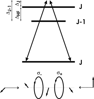
FIG. 1.: Schematic setup of the gray optical lattice.

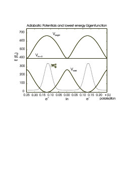
FIG. 2.: Adiabatic potentials $V_{\mbox{dark}}$, $V_{\mbox{bright}}$ and $V_{m=0}$ (solid curves) and the atomic position distribution of the lowest energy eigenfunction $\psi_{g}$ shifted by the corresponding eigenenergy (dashed line) for the $J_{g}=1\to J_{e_{j}}=1,0$ system for $U_{1}=400\,E_{R}$ and $U_{0}=400\,E_{R}$.

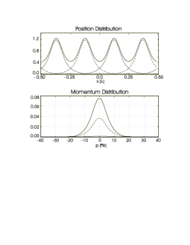
FIG. 3.: Position and momentum distribution for $U_{1}=200\,E_{R}$, $U_{0}=100\,E_{R}$, $\Gamma_{1}=3\,E_{R}/\hbar$ and $\Gamma_{0}=1\,E_{R}/\hbar$ for the $J_{g}=1\to J_{e_{j}}=1,0$ system. The uppermost lines give the total distributions, while the lower lines give the partial contributions of the various Zeeman substates. The dotted curves correspond to the $m=0$ substate. The momentum distribution is normalized and given in units of $(\hbar k)^{-1}$, the position distribution is periodic and given in arbitrary units.

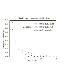
FIG. 4.: Population of the low energy eigenstates for the $J_{g}=2\to J_{e_{j}}=2,1$ system for various lightshifts $U_{2}$ and ratios of the optical pumping rates $\Gamma_{1}/\Gamma_{2}$

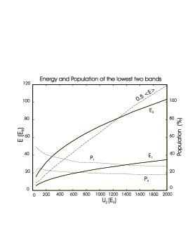
FIG. 5.: Ground $P_{1}$ and first excited band $P_{2}$ populations (short dashed curves), the corresponding energies $E_{1}$, $E_{2}$ and the mean energy $\langle E\rangle$ (dot dashed line) for the $J_{g}=2\to J_{e_{j}}=2,1$ system as a function of the laser intensity $\propto U_{2}$ for fixed ratios of the lightshift potentials $U_{1}/U_{2}=1/3$ and of the optical pumping rates $\Gamma_{1}/\Gamma_{2}=0.1$.

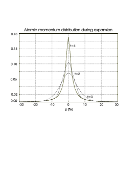
FIG. 6.: Normalized atomic momentum distribution during various stages of the field turnoff $t=0$, $t=2\,\tau_{R}$ and $t=4\,\tau_{R}$ for a $J_{g}=1\to J_{e_{j}}=1,0$ system and for the same parameters as in Fig. 3. The optical potential decreases as $U_{J\!e_{j}}(t)=U_{J\!e_{j}}(0)exp(-{1\over 2}(t/\tau_{R})^{2})$. The units on the vertical axis are $(\hbar k)^{-1}$.

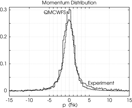
FIG. 7.: Normalized momentum distribution of the atoms after their adiabatic release from the lattice. The QMCWF simulation corresponds to the solid line, while the dashed line gives the corresponding experimental result for $\Delta_{3}=26\,\gamma_{3}$ and $U_{3}=\gamma_{3}/4$. The units on the vertical axis are $(\hbar k)^{-1}$.

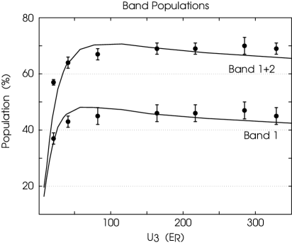
FIG. 8.: Population of the lowest (lower curve) and lowest two (upper curve) bands of the optical lattice as a function of the lightshift as obtained by quantum rate equations (solid lines) in comparison to the experimentally measured results (data points) for the $J_{g}=3\to J_{e_{j}}=3,2$ transition of the ⁸⁵Rb $D_{1}$-line. The detuning was chosen to be $\Delta_{3}=26\,\gamma_{3}$ to the blue of the $J_{g}=3\to J_{e_{1}}=3$ transition.

REFERENCES

- [1] M. H. Anderson et al., Science 269, 198 (1995).
- [2] C. C. Bradley et al., Phys. Rev. Lett. 75, 1687 (1995).
- [3] K. B. Davis et al., Phys. Rev. Lett. 75, 3969 (1995).
- [4] A. Aspect et al., Phys. Rev. Lett.61, 826 (1988).
- [5] J. Lawall et al., Phys. Rev. Lett. 75, 4194 (1995).
- [6] T. Esslinger et al., Phys. Rev. Lett 76, 2432 (1996).
- [7] M. Kasevich and S. Chu, Phys. Rev. Lett.69, 1741 (1992).
- [8] J. Chen et al., Phys. Rev. Lett. 69, 1344 (1992).
- [9] A. Kastberg et al., Phys. Rev. Lett. 74, 1542 (1995).
- [10] T. Esslinger et al., Opt. Lett. 21, 991 (1996).
- [11] R. Dum et al., Phys. Rev. Lett. 73, 2829 (1994).
- [12] T. Pellizzari and H. Ritsch, Europhys. Lett. 31 , 133 (1995).
- [13] H. J. Lee et al., Phys. Rev. Lett. 76, 2658 (1996).
- [14] M. G. Prentiss, Science 260, 1078 (1993); G. P. Collins, Phys. Today 46, 17 (1993), and Refs. therein.
- [15] G. Grynberg and J.-Y. Courtois, Europhys. Lett, 27, 41 (1994).
- [16] K.I. Petsas et al., Phys. Rev. A 53, 2533 (1996).
- [17] A. Hemmerich et al., Phys. Rev. Lett. 75, 37 (1995).
- [18] The optical lattice described in Ref. [10] is induced by coupling a ground state with angular momentum J to two excited states with angular momenta and . For this case the localized atoms are off-resonantly coupled to the excited state with angular momentum and decoupled from the excited state with angular momentum .
- [19] It is also possible to build up the lattice structure with two laser fields, each coupling one of the two excited states to the ground state. The frequency difference between this two fields should be small, so that their relative phase mismatch can be ignored over the size of the experimental setup. Otherwise one obtains an additional superlattice structure [12, 27].
- [20] P. Marte et al., Phys. Rev. A 47, 1378 (1993)
- [21] This assumption is not essential here and might not be the experimentally optimal case, but it greatly reduces the calculational effort.
- [22] Y. Castin and J. Dalibard, Europhys. Lett. 14, 761 (1991).
- [23] see e.g. K. Ellinger, J. Cooper and P. Zoller, Phys. Rev. A 49, 3909 (1995), and Refs. therein.
- [24] E. V. Goldstein et al., Phys. Rev. A 53, 2604 (1996)
- [25] R. C. J. Spreuuw, Europhys. Lett. 32, 469 (1995).
- [26] H. M. Wiseman and M. J. Collet, Phys. Lett. A 202, 246 (1996).
- [27] R. Grimm , J. Söding and Yu. B. Ovchinikov, JETP. Lett. 61, 5 (1995).