The Normalized Radial Basis Function Neural Network and its Relation to the Perceptron

Abstract

The normalized radial basis function neural network emerges in the statistical modeling of natural laws that relate components of multivariate data. The modeling is based on the kernel estimator of the joint probability density function pertaining to given data. From this function a governing law is extracted by the conditional average estimator. The corresponding nonparametric regression represents a normalized radial basis function neural network and can be related with the multi-layer perceptron equation. In this article an exact equivalence of both paradigms is demonstrated for a one-dimensional case with symmetric triangular basis functions. The transformation provides for a simple interpretation of perceptron parameters in terms of statistical samples of multivariate data.

I Introduction

Multi-layer perceptrons (MLP) have played a central role in the research of neural networks [1, 2]. Their study began with the nonlinear and adaptive response characteristics of neurons, which have brought with them many difficulties related to the understanding of the collective properties of MLPs. Consequently, it was discovered rather late that the MLP is a universal approximator of relations between input signals [1, 2, 3]. However, supervised training of MLPs by back-propagation of errors is relatively time-consuming and does not provide a simple interpretation of MLP parameters. The inclusion of a priori information into an MLP is also problematic. Many of these problems do not appear in simulations of radial basis function neural networks (RBFN) [4]. The structure of the normalized RBFN stems from the representation of the empirical probability density function of sensory signals in terms of prototype data and can simply be interpreted statistically [5]. An optimal description of relations is described in this case by the conditional average estimator (CA), which represents a general, non-linear regression and corresponds to a normalized RBFN. A priori information can also be included in this model by initialization of prototypes. A learning rule derived from the maximum entropy principle describes a self-organized adaptation of neural receptive fields [5, 6, 7]. The separation of input signals into independent and dependent variables need not be done before training, as with MLPs, but it can be performed when applying a trained network. Because of these convenient properties of RBFNs, our aim was to compare both NN paradigms and to explore whether RBFN is equivalent to MLP with respect to modeling of mapping relations. Here we demonstrate their exact equivalence for a simple one-dimensional case by showing that the mapping relation of an RBFN can be directly transformed into that of an MLP, and vice versa. This further indicates how MLP parameters can also be statistically interpreted in the case of multivariate data.

II Estimation of probability density functions

The task of both paradigms is the modeling of relations between components of measured data. We assume that $D$ sensors provide signals $(s_{1},s_{2},\ldots,s_{D})$ that comprise a vector ${\bf x}$. The modeling is here based on an estimation of the joint probability density function (PDF) of vector ${\bf x}$. We assume that information about the probability distribution is obtained by a repetition of measurements that yield $N$ independent samples $\{{\bf x}_{1},{\bf x}_{2},\ldots,{\bf x}_{N}\}$. The PDF is then described by the kernel estimator [6]:

$$f_{e}({\bf x})={1\over N}\sum_{n=1}^{N}w({\bf x}-{\bf x}_{n},\sigma)$$ (1)

Here the kernel $w({\bf x}-{\bf x}_{n},\sigma)$ is a smooth approximation of the delta function, such as a radially symmetric Gaussian function $w({\bf x},\sigma)={\rm const.}~{}\exp(-\parallel{\bf x}\parallel^{2}/2\sigma^{2})$. The constant $\sigma$ can be objectively interpreted as the width of a scattering function describing stochastic fluctuations in the channels of a data acquisition system and can be determined by a calibration procedure [5, 7, 8].

However, in an application the complete PDF need not be stored; it is sufficient to preserve a set of statistical samples ${\bf x}_{n}$. In order to obtain a smooth estimator of the PDF, the neighboring sample points should be separated in the sample space by approximately $\sim\sigma$. From this condition one can estimate a proper number $N$ of samples [5, 7, 8]. In a continuous measurement the number of samples increases without limit, and there arises a problem with the finite capacity of the memory in which the data are stored. Neural networks are composed of finite numbers of memory cells, and therefore we must assume that the PDF can be represented by a finite number $K$ of prototype vectors $\{{\bf q}_{1},{\bf q}_{2},\ldots,{\bf q}_{K}\}$ as

$$f_{r}({\bf x})={1\over K}\sum_{k=1}^{K}w({\bf x}-{\bf q}_{k},\sigma)$$ (2)

In the modeling of $f_{r}$ the prototypes are first initialized by $K$ samples: $\{{\bf q}_{k}={\bf x}_{k}~{},~{}k=1\ldots K\}$, which represent a priori given information. These prototypes can be adapted to additional samples ${\bf x}_{N}$ in such a way that the mean-square difference between $f_{e}$ and $f_{r}$ is minimized. The corresponding rule was derived elsewhere, and it describes the self-organized unsupervised learning of neurons, each of which contains one prototype ${\bf q}_{k}$ [6, 7].

The estimator of the PDF given in Eq.  2 can be simply generalized by assuming that various prototypes are associated with different probabilities and receptive fields [7]: ${1/K}\mapsto p_{k}$ and $\sigma\mapsto\sigma_{k}$. This substitution yields a generalized model:

$$f_{g}({\bf x})=\sum_{k=1}^{K}p_{k}\,w({\bf x}-{\bf q}_{k},\sigma_{k})$$ (3)

However, in this case several advantages of a simple interpretation of the model Eq.  2 are lost, which causes problems when analyzing its relation to the perceptron model. Therefore, we further consider the simpler model given in Eq.  2.

III Conditional average

In the application of an adapted PDF the information must be extracted from prototypes, which generally corresponds to some kind of statistical estimation. In a typical application there is some partial information given, for instance the first $i$ components of the vector: ${\bf g}=(s_{1},s_{2},..,s_{i},\emptyset)$, while the hidden data, which have to be estimated, are then represented by the vector ${\bf h}=(\emptyset,s_{i+1},..,s_{D})$ [5, 8]. Here $\emptyset$ denotes the missing part in a truncated vector. As an optimal estimator we apply the conditional average, which can be expressed by prototype vectors as [4, 5, 8]:

$$\widehat{\bf h}=\sum_{k=1}^{K}B_{k}({\bf g}){\bf h}_{k},$$ (4)

where

$$B_{k}({\bf g})=\frac{w({\bf g}-{\bf g}_{k},\sigma)}{\sum_{j=1}^{K}w({\bf g}-{\bf g}_{j},\sigma)}.$$ (5)

Here the given vector ${\bf g}$ plays the role of the given condition. The basis functions $B_{k}({\bf g})$ are strongly nonlinear and peaked at the truncated vectors ${\bf g}_{k}$. They represent the measure of similarity between the given vector ${\bf g}$ and the prototypes ${\bf g}_{k}$.

The CA represents a general non-linear, non-parametric regression, which has already been successfully applied in a variety of fields [5, 7, 8]. It is important that selection into given and hidden data can be done after training the network, which essentially contributes to the adaptability of the method to various tasks in an application [5].

The CA corresponds to a mapping relation ${\bf g}\rightarrow{\bf h}$ that can be realized by a two-layer RBFN [4]. The first layer consists of $K$ neurons. The $k$-th neuron obtains the input signal ${\bf g}$ over synapses described by ${\bf g}_{k}$ and is excited as described by the radial basis function $B_{k}({\bf g})$. The corresponding excitation signal is then transferred to the neurons of the second layer. The $i$-th neuron of this layer has synaptic weights $h_{k,i}$ and generates the output $\widehat{h}_{i}({\bf g})$.

IV Transition from RBFN to MLP

In order to obtain a relation with an MLP it is instructive to analyze the performance of the RBFN in a simple two-dimensional case, for example as shown in Fig. 1. We consider the function $y(x)$ described by a set of sample pairs $\{x_{1},y_{1};\ldots x_{i},y_{i};\ldots;x_{N},y_{N}\}$ with constant spacing between the sample points: $\triangle x=x_{j+1}-x_{j}~{}{\rm for}~{}j=1\ldots N-1$. We further introduce a triangular and a piecewise linear sigmoidal basis function, as shown in Fig. 2:

$$B_{i}(x)=\{ 1 -\quad{|x-x_{i}|\over\triangle x}\quad\ldots\quad{\rm for}~{}x_{i-1}<x<x_{i+1}~{};~{}$$ (6)

$$0 \ldots\quad{\rm elsewhere}\quad\}$$

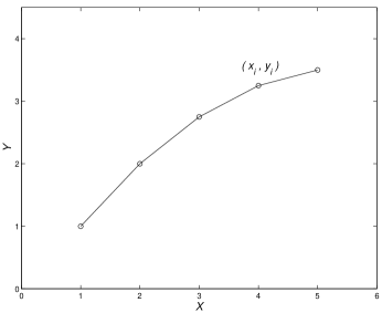
Figure 1: An example of a linear interpolating function through sample points.

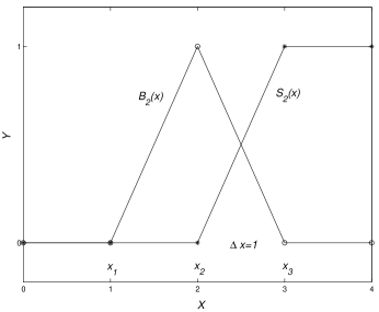
Figure 2: Examples of a triangular and a piecewise linear sigmoidal basis functions.

$$S_{i}(x)=\{ 0 ~{}\ldots\quad{\rm for}~{}x<x_{i}~{};~{}$$ (7)

$$(x-x_{i})/\triangle x ~{}\ldots\quad{\rm for}~{}x_{i}\leq x\leq x_{i+1}~{};~{}$$

$$1 ~{}\ldots\quad{\rm for}~{}x>x_{i+1}\quad\}$$

Using these, we can represent the function $y(x)$ by a linear interpolating function comprising straight line segments connecting the sample points. The CA can in this case be readily transformed into an MLP expression by utilizing the relations:

$$B_{i+1}(x)=S_{i}(x)-S_{i+1}(x)$$ (8)

$$S_{i}(x)={B_{i+1}(x)\over B_{i}(x)+B_{i+1}(x)}$$ (9)

The result is:

$$\widehat{y}(x) = {y_{1}B_{1}(x)+\ldots+y_{N}B_{N}(x)\over B_{1}(x)+\ldots+B_{N}(x)}$$ (10)

$$= {y_{1}B_{1}(x)\over B_{1}(x)+\ldots+B_{N}(x)}+\ldots+{y_{N}B_{N}(x)\over B_{1}(x)+\ldots+B_{N}(x)}$$

$$= {y_{1}B_{1}(x)\over B_{1}(x)+B_{2}(x)}+y_{2}B_{2}(x)+\ldots$$

$$\ldots+y_{N-1}B_{N-1}(x)+{y_{N}B_{N}(x)\over B_{N-1}(x)+B_{N}(x)}$$

In the denominator of the first and last terms of this expression, only those basis functions are kept that differ from zero in the region where the basis function in the numerator also differs from zero. The denominator in terms of index $2$ to $N-1$ is $1$ because of the overlapping of neighboring basis functions. We insert relations of Eq. (8,9) into Eq. (10) and obtain

$$\widehat{y}(x)=y_{1}+\sum_{i=1}^{N-1}(y_{i+1}-y_{i})\;S_{i}(x)$$ (11)

By introducing the parameters: $\triangle y_{i}=y_{i+1}-y_{i},\quad c_{i}=1/(x_{i+1}-x_{i}),\quad\Theta_{i}=x_{i}/(x_{i+1}-x_{i})$  and a unique, normalized sigmoidal basis function:

$$S(x)=\{ 0 \ldots~{}{\rm for}~{}x<0~{};~{}$$ (12)

$$x \ldots~{}{\rm for}~{}0\leq x\leq 1~{};~{}$$

$$1 \ldots~{}{\rm for}~{}x>1\quad\}$$

we can write Eq. (11) in the form of a two-layer perceptron mapping relation

$$\widehat{y}(x)=y_{1}+\sum_{i=1}^{N-1}\triangle y_{i}\,S(c_{i}x-\Theta_{i})$$ (13)

The first layer corresponds to neurons with synaptic weights $c_{i}$ and threshold values $\Theta_{i}$, while the second layer contains a linear neuron with synaptic weights $\triangle y_{i}$ and threshold $y_{1}$.

The above derivation demonstrates that for the two-dimensional distribution the mapping $x\rightarrow y$ determined by the conditional average is identical with the mapping relation of a multi-layer perceptron. However, a difference appears when the operations needed for the mapping are executed. The operators involved in both cases are described by different basis functions, which correspond to different neurons in the implementation. If the prototypes are not evenly spaced, then the last equation can still be applied, although the transition regions will be of different spans. However, in this case the basis functions $B_{i}(x)$ are no longer symmetric. In applications it is more convenient to use a Gaussian basis function rather than a triangular one, and in the perceptron expression this yields the function $\tanh(\ldots)$. In this case, the estimated function $\widehat{y}(x)$ generally does not run through the sample points but rather approximates them by a function having a more smooth derivative than the piecewise linear function. In this case, the correspondence between RBFN and MLP is not exact but approximate.

An additional interpretation is needed when the data are not related by a regular function $y(x)$ but randomly, as described by a joint probability density function $f(x,y)$. In this case, various values of $y$ can be observed at a given $x$. Evaluation of CA in this case is not problematic, while in the perceptron relation Eq. (13) the value $y_{i}$ must be substituted by the conditional average of variable $y$ at $x_{i}$.

The analysis of the correspondence between RBFN and MLP can be extended to multi-variate mappings. Let us first consider the situation with just two prototypes ${\bf q}_{i}$ and ${\bf q}_{j}$ and Gaussian basis functions. The CA is then described by the function

$$\widehat{\bf h}({\bf g})={{\bf h}_{i}\exp({-\parallel{\bf g}-{\bf g}_{i}\parallel^{2}\over 2\sigma^{2}})+{\bf h}_{j}\exp({-\parallel{\bf g}-{\bf g}_{j}\parallel^{2}\over 2\sigma^{2}})\over\exp({-\parallel{\bf g}-{\bf g}_{i}\parallel^{2}\over 2\sigma^{2}})+\exp({-\parallel{\bf g}-{\bf g}_{j}\parallel^{2}\over 2\sigma^{2}})}$$ (14)

We introduce the notation: ${\bf g}_{i}=\overline{\bf g}-\triangle{\bf g}~{},~{}{\bf g}_{j}=\overline{\bf g}+\triangle{\bf g}~{},~{}{\bf h}_{i}=\overline{\bf h}-\triangle{\bf h}~{},~{}{\bf h}_{j}=\overline{\bf h}+\triangle{\bf h}$  in which the overline denotes the average value and $2\triangle{\bf g}$ is the spacing of the prototypes. If we express the norm by a scalar product and cancel the term $\exp[-(\parallel{\bf g}-\overline{\bf g}\parallel^{2}+\parallel\triangle{\bf g}\parallel^{2})/2\sigma^{2})$ in the numerator and denominator, we obtain the expression:

$$\widehat{\bf h}({\bf g})=\overline{\bf h}+\triangle{\bf h}\tanh\left[\triangle{\bf g}\cdot({\bf g}-\overline{\bf g})/\sigma^{2}\right]$$ (15)

in which $\cdot$ denotes the scalar product. In order to obtain the relation between RBFN and MLP, we introduce a weight vector ${\bf c}=\triangle{\bf g}/\sigma^{2}$ and a threshold value $\Theta=\overline{\bf g}\cdot\triangle{\bf g}/\sigma^{2}$ into Eq. (15) and obtain:

$$\widehat{\bf h}({\bf g})=\overline{\bf h}+\triangle{\bf h}\tanh\left[{\bf c}\cdot({\bf g}-\overline{\bf g})-\Theta\right]$$ (16)

This expression again describes a two-layer perceptron: the first layer is composed of one neuron having the synaptic weights described by the vector ${\bf c}$ and the threshold value $\Theta$. The second layer is composed of linear neurons having synaptic weights $\triangle h_{i}$ and threshold values $\overline{h_{i}}$.

The first-order approximation of the mapping expression Eq.  16 is :

$$\widehat{\bf h}({\bf g})=\overline{\bf h}+\triangle{\bf h}\triangle{\bf g}\cdot({\bf g}-\overline{\bf g})/\sigma^{2}$$ (17)

This equation represents a linear regression of ${\bf h}$ on ${\bf g}$ that runs through both prototype points if we assign $\sigma^{2}=\parallel\triangle{\bf g}\parallel^{2}$. Its slope is determined by the covariance matrix ${\bf\Sigma}=\triangle{\bf h}\triangle{\bf g}^{\rm T}$. However, the nonlinear regression specified in Eq. (15) follows a linear regression only in the vicinity of a point determined by $\overline{\bf g}$ and $\overline{\bf h}$ while it exhibits saturation when ${\bf g}$ runs from $\overline{\bf g}$ over given prototypes to infinity. The saturation is a consequence of the function $\tanh(\ldots)$, which is basic in the modeling of a multi-layered perceptron.

The reasoning presented above for a multi-variate case requires additional explanation when transferred to a situation consisting of many prototypes. Let us assume that $N$ prototypes with indexes $1\ldots N$ can be found in the hyper-sphere of radius approximately $\sigma$ around the given datum ${\bf g}$, and let these prototypes be spaced by approximately equal distances. The CA can now be expressed with leading terms and remainders as follows :

$$\widehat{\bf h}({\bf g})={\sum_{i=1}^{N}{\bf h}_{i}\exp(-\parallel{\bf g}-{\bf g}_{i}\parallel^{2}/2\sigma^{2})\over\sum_{i=1}^{N}\exp(-\parallel{\bf g}-{\bf g}_{i}\parallel^{2}/2\sigma^{2})+O_{w}}+O_{h}$$ (18)

Here $O_{h}$ and $O_{w}$ represent two remainders, which are small in comparison with the two leading terms. We again introduce the average value, but now with respect to $N$ prototypes: ${\bf g}_{i}=\overline{\bf g}+\triangle{\bf g}_{i}~{},~{}{\bf h}_{i}=\overline{\bf h}+\triangle{\bf h}_{i}~{}{\rm for}~{}i=1\ldots N$. With this we obtain the approximate expression :

$$\widehat{\bf h}({\bf g})\cong\overline{\bf h}+{\sum_{i=1}^{N}\triangle{\bf h}_{i}\exp[\triangle{\bf g}_{i}\cdot({\bf g}-\overline{\bf g})/\sigma^{2}]\over\sum_{i=1}^{N}\exp[\triangle{\bf g}_{i}\cdot({\bf g}-\overline{\bf g})/\sigma^{2}]}$$ (19)

For ${\bf g}$ in the vicinity of the average value, a linear approximation of the exponential function is applicable, which yields

$$\widehat{\bf h}({\bf g})\cong\overline{\bf h}+{1\over N}\sum_{i=1}^{N}\triangle{\bf h}_{i}\triangle{\bf g}_{i}\cdot({\bf g}-\overline{\bf g})/\sigma^{2}$$ (20)

This expression represents a linear regression of ${\bf h}$ on ${\bf g}$ specified by $N$ points. If we express the covariance matrix

$${\bf\Sigma}={1\over N}\sum_{i=1}^{N}\triangle{\bf h}_{i}\triangle{\bf g}_{i}^{\rm T}$$ (21)

by two principal vectors $\triangle{\bf h}_{p}$ and $\triangle{\bf g}_{p}$ :

$${\bf\Sigma}=\triangle{\bf h}_{p}\triangle{\bf g}_{p}^{\rm T}$$ (22)

we obtain a simplified expression of the linear regression

$$\widehat{\bf h}({\bf g})\cong\overline{\bf h}+\triangle{\bf h}_{p}\triangle{\bf g}_{p}\cdot({\bf g}-\overline{\bf g})/\sigma^{2}$$ (23)

which is an approximation of an MLP mapping relation

$$\widehat{\bf h}({\bf g})\cong\overline{\bf h}+\triangle{\bf h}_{p}\tanh[\triangle{\bf g}_{p}\cdot({\bf g}-\overline{\bf g})/\sigma^{2}]$$ (24)

The parameters of a single neuron in the perceptron expression thus correspond to the principal vectors of the covariance matrix ${\bf\Sigma}=\triangle{\bf h}_{p}\triangle{\bf g}_{p}^{\rm T}$ determining a local regression around the center of several neighboring prototypes.

The above expression shows that the transition from RBFN to MLP can be quite generally performed. However, in the multi-variate case, the decomposition of CA into a perceptron mapping is not as simple as in the one-dimensional case, because the interpretation of perceptron parameters goes over local regression determined by various prototypes surrounding the given datum ${\bf g}$. In spite of this, our conjecture is that both paradigms are equivalent with respect to the statistical modeling of mapping relations, provided that both models include the same number of adaptable parameters.

V Conclusion

The conditional average representing a linear interpolating function by the regular function $y(x)$ shown in Fig. 1 can be exactly decomposed into the multilayer perceptron relation. When there are a small number of noise-corrupted sample data points representing the function, the question of proper smoothing arises. In the case of CA this is done by using symmetric radial basis functions and increasing their width. The basis functions centered at various points then overlap, which results in a smoother $\widehat{y}(x)$. Because of multiple overlapping, the relations between radial basis and sigmoidal functions becomes more complicated, and the transition between the conditional average and the perceptron relation becomes less obvious. However, when the prototypes are obtained by self-organization, they represent a statistical regularity, and the CA generally does not exhibit statistical fluctuations. In this case, the proper RBF width corresponds to the distance between closest neighbors, and additional smoothing is not needed. The corresponding parameters of the perceptron for one-dimensional mapping can then be simply interpreted in terms of prototypes, as described by the model equations Eq. 4 and Eq. 24. However, due to the complexity of the self-organized formation of prototypes determining the RBFN and the back-propagation learning of the MLP, it would be difficult to find an exact mapping relation between both models, especially in the multivariate case.

References

- [1] S. Haykin, Neural Networks, A Comprehensive Foundation, 2nd ed. New York, NY: Macmillan, 1999.
- [2] R. Hecht-Nielsen, Neurocomputing, Reading, MA: Addison-Wesley, 1990.
- [3] G. Cybenko, ”Approximations by Superpositions of a Sigmoidal Function,” Math. Cont., Sig. & Syst., vol. 2, pp. 303-314, 1989.
- [4] C. M. Bishop, ”Neural Networks and their Applications,” Rev. Sci. Instr., vol. 65, pp. 1830-1832, 1994.
- [5] I. Grabec and W. Sachse, Synergetics of Measurement, Prediction and Control, Berlin: Springer-Verlag, 1997.
- [6] I. Grabec, ”Self-Organization of Neurons Described by the Maximum Entropy Principle,” Biological Cybernetics, vol. 69 (9), pp. 403-409, 1990.
- [7] I. Grabec, ”Experimental Modeling of Physical Laws,” Eur. Phys. J. B, vol. 22, pp. 129-135, 2001.
- [8] I. Grabec, ”Extraction of Physical Laws from Joint Experimental Data,” Eur. Phys. J. B, vol. 48, pp. 279-289, 2005.
- [9] R. O. Duda and P. E. Hart, Pattern Classification and Scene Analysis, New York: J. Wiley and Sons, 1973, Ch. 4.