Kinetically-balanced Gaussian Basis Set Approach to Relativistic Compton Profiles of Atoms

Abstract

Atomic Compton profiles (CPs) are a very important property which provide us information about the momentum distribution of atomic electrons. Therefore, for CPs of heavy atoms, relativistic effects are expected to be important, warranting a relativistic treatment of the problem. In this paper, we present an efficient approach aimed at ab initio calculations of atomic CPs within a Dirac-Hartree-Fock (DHF) formalism, employing kinetically-balanced Gaussian basis functions. The approach is used to compute the CPs of noble gases ranging from He to Rn, and the results have been compared to the experimental and other theoretical data, wherever possible. The influence of the quality of the basis set on the calculated CPs has also been systematically investigated.

I Introduction

Recent years have seen tremendous amount of progress in the field of relativistic electronic structure calculations of atoms and molecules using Dirac-equation-based approachesdirac-gen . Particularly noteworthy are the advances made in the field of basis-set-based relativistic electronic structure theory pioneered by Kimkim , and Kagawakagawa . Although, initially, the basis-sets employed in the calculations were of the ordinary Slater-typekim ; kagawa , however, now-a-days, the preferred basis functions are those which incorporate the so-called kinetic-balance condition between the large and the small component basis functionsishikawa ; dyall ; kbgf . The most commonly used variety of such functions in relativistic electronic-structure calculations are the kinetically-balanced Gaussian functions (KBGFs) which have not only been instrumental in avoiding the problem of ’variational collapse’, but have also allowed the import of efficient algorithms developed in basis-set-based nonrelativistic quantum chemistry. Using such basis functions, calculations are now routinely performed both at the mean-field Hartree-Fock (henceforth Dirac-Hartree-Fock (DHF)) levelcal-at-dhf ; cal-mol-dhf , as well as at the correlated level, employing methods such as the configuration-interaction (CI) approach, both for atomsci-shukla , and moleculesci-relmol .

However, the progress in calculating wave functions and atomic energies using KGBFs has not been matched by the progress in computing expectation values corresponding to various physical quantities. For example, atomic Compton profiles (CPs) are a very important property which provide us information about the momentum distribution of atomic electrons, and help us in interpreting the x-ray Compton scattering data from atoms in the large momentum-transfer regimecompton-review . Compton profiles are also very useful in understanding the bonding properties, as one makes a transition from the atomic scale to the scale of condensed mattercompton-review . Indeed, the nonrelativistic Schrödinger equation based calculations of CPs of atomic and molecular systems both within an ab initio, as well as model-potential based, formalisms are quite well developedcompton-review . As recently demonstrated by us, and several other authors earlier on, that such nonrelativistic ab initio calculations of CPs can also be performed on crystalline systemswannier . However, for systems involving heavy atoms, on intuitive grounds one expects that the relativistic effects will become quite important, thereby requiring a relativistic treatment of the problemkane-review . Long time back Mendelsohn et al.rel-com-prof , and Bigss et al.rel-comp-prof-2 presented the first fully-relativistic calculations of atomic CPs which were performed at the DHF level, employing a finite-difference based numerical approach. Yet, since that time, there has been hardly any activity in the field, which is surprising given the fact that now relativistic electronic structure calculations are routinely performed employing KBGF basis functions. Therefore, in this work, our aim is to report the first calculations of atomic CPs at the DHF level, employing a basis set composed of KBGFs. Our approach is based upon analytic formulas for the CP matrix elements with respect to a KBGF basis set, whose derivation is presented in the Appendix. The DHF calculations of atomic CPs are presented for the entire rare gas series (He to Rn), and our results are compared to experimental data, wherever available. Additionally, our results for Ar, Kr, Xe, and Rn are also compared to the DHF results of Mendelsohn et al.rel-com-prof , and Bigss et al.rel-comp-prof-2 , and excellent agreement is obtained between the two sets of calculations.

At this point we would like to clarify one important aspect related to the relativistic effects which our calculations are computing, in light of the fact that there have been several papers in the literature dealing with a relativistic treatment of Compton scattering of bound electronsribber ; holm ; berg . Several authors have pointed out that for very large photon energies, a fully relativistic treatment, within the framework of quantum-electrodynamics, of the Compton scattering from bound electrons is essentialkane-review . When such a treatment of the problem is performed, it is not clear whether the Compton scattering cross-sections can at all be written in terms of Compton profilesribber ; holm ; kane-review ; berg . Our work presented here, however, does not correspond to that regime of photon energies. What we mean by the relativistic effects here are the changes in the computed CPs because of a relativistic treatment of the bound electrons within a Dirac Hamiltonian based formalism. Thus, our calculations assume that the Compton scattering from atomic electrons can be described in terms of the CPs under the impulse approximationimpuse . The electron momentum densities needed to calculate the CPs, however, are computed from the Dirac orbitals of the atomic electrons. This approach is identical to the one adopted in the earlier DHF calculationsrel-com-prof ; rel-comp-prof-2 .

The remainder of this paper is organized as follows. In section II we present the basic theoretical formalism behind the present set of calculations. Next in section III we present and discuss the results of our calculations. Finally, in section IV our conclusions, as well as possible future directions for further work are discussed. Additionally, in the Appendix we present the derivation of the closed-form formulas for CPs over KBGFs, used in our calculations.

II Theory

Our theory is based upon the Dirac-Coulomb Hamiltonian

$$H=\sum_{i}(c{\bf\alpha}_{i}\cdot{\bf p}_{i}+c^{2}(\beta_{i}-1)+V_{\mbox{nuc}}(r_{i}))+\sum_{i<j}\frac{1}{r_{ij}},$$ (1)

where $c$ is the speed of light, ${\bf p}$ is the momentum operator, $V_{\mbox{nuc}}(r)$ is the electron-nucleus interaction potential, indices $i$ and $j$ label the electrons of the atom, and $r_{ij}$ is the distance between the $i$th and $j$th electrons. For $V_{\mbox{nuc}}(r)$ a spherical finite-nucleus approximation is employed, with the radius estimated as $2.2677\times 10^{-5}A^{1/3}$, where $A$ is the atomic mass numbercal-at-dhf . The Dirac matrices are chosen to be ${\bf\alpha}=\left(\begin{array}[]{cc}{\bf 0}&{\bf\sigma}\\ {\bf\sigma}&{\bf{\bf 0}}\end{array}\right)$ and $\beta=\left(\begin{array}[]{ll}{\bf I}&{\bf 0}\\ {\bf 0}&{\bf-I}\end{array}\right)$, where ${\bf 0}$, ${\bf I}$, and ${\bf\sigma}$, represent the 2$\times$2 null, identity and Pauli matrices, respectively. Eq. (1) is solved under the DHF approximation utilizing spherical symmetry with the orbitals of the form

$$\psi_{n\kappa m}=r^{-1}\left(\begin{array}[]{l}P_{n\kappa}(r)\chi_{\kappa m}(\theta,\phi)\\ iQ_{n\kappa}(r)\chi_{-\kappa m}(\theta,\phi)\end{array}\right),$$ (2)

where $P_{n\kappa}(r)$ and $Q_{n\kappa}(r)$ are the radial large and small components, and $\chi_{\kappa m}(\theta,\phi)$ is the two-component angular part composed of Clebsch-Gordon coefficients and spherical harmonics. In the basis-set approach adopted here, the radial parts of the wave function are expressed as linear combination of radial Gaussian type of functions

$$P_{n\kappa}(r)=\sum_{i}C_{\kappa i}^{L}g_{\kappa i}^{L}(r),$$

and

$$Q_{n\kappa}(r)=\sum_{i}C_{\kappa i}^{S}g_{\kappa i}^{S}(r),$$

where $C_{\kappa i}^{L}$ and $C_{\kappa i}^{S}$, are the expansion coefficients of the large and small component basis functions, respectively. The large-component basis function is given by

$$g_{\kappa i}^{L}(r)=N_{\kappa i}^{L}r^{n_{\kappa}}e^{-\alpha_{i}r^{2}},$$ (3)

while the small-component basis function is obtained by the kinetic-balancing conditionkbgf

$$g_{\kappa i}^{S}=N_{\kappa i}^{S}(\frac{d}{dr}+\frac{\kappa}{r})g_{\kappa i}^{L}(r).$$ (4)

Above $n_{\kappa}$ is the principal quantum number associated with a symmetry species ($n_{\kappa}=1,2,2,3,3,\ldots$, for symmetry species $s$, $p_{1/2}$, $p_{3/2}$, $d_{3/2}$, $d_{5/2}$, $\ldots$), $\alpha_{i}$ is the Gaussian exponent of the $i$th basis function, and $N_{\kappa i}^{L}$, $N_{\kappa i}^{S}$ are the normalization coefficients associated with the large and the small component basis functions, respectively.

Under the impulse approximationimpuse , the differential cross-section of Compton scattering of x-rays from many-electron systems is proportional to the Compton profile

$$J(q)=\int\int dp_{x}dp_{y}\rho({\bf p}),$$ (5)

where $\rho({\bf p})$ is the momentum distribution of the electrons before scattering and $q$ is the component of the momentum of the electron along the scattering vector, assumed to be along the $z$ direction. Under the mean-field DHF approximation, for a closed-shell atom, the expression for the CP reduces to

$$J(q)=\sum(2j_{i}+1)J_{n_{i}\kappa_{i}}(q),$$ (6)

where $j_{i}$ is the total angular momentum of the $i$th orbital while, $J_{n_{i}\kappa_{i}}$ is the CP associated with it

$$J_{n_{i}\kappa_{i}}(q)=\frac{1}{2}\int_{q}^{\infty}\{|P_{n_{i}\kappa_{i}}(p)|^{2}+|Q_{n_{i}\kappa_{i}}(p)|^{2}\}pdp,$$ (7)

where $P_{n_{i}\kappa_{i}}(p)$ and $Q_{n_{i}\kappa_{i}}(p)$ are the Fourier transforms of the radial parts of the large and small components, respectively, of the $i$th occupied orbital (cf. Eq. (2)) and are defined as

$$P_{n_{i}\kappa_{i}}(p)=\frac{4\pi}{(2\pi)^{3/2}}\int_{0}^{\infty}rP_{n_{i}\kappa_{i}}(r)j_{l_{A}}(pr)dr,$$ (8)

and

$$Q_{n_{i}\kappa_{i}}(p)=\frac{4\pi}{(2\pi)^{3/2}}\int_{0}^{\infty}rQ_{n_{i}\kappa_{i}}(r)j_{l_{B}}(pr)dr,$$ (9)

where $j_{l_{A}}(pr)$($j_{l_{B}}(pr)$) is the spherical Bessel function corresponding to the orbital angular momentum $l_{A}$($l_{B}$) of the large (small) component. Therefore, calculation of atomic CPs involves computation of two types of integrals: (i) radial Fourier Transforms of Eqs. (8) and (9), and (ii) momentum integrals of the Fourier transformed orbitals in Eq. (7). When one solves the DHF equation for atoms using the finite-difference techniques, then, obviously the calculation of atomic CPs mandates that both these types integrals be computed by means of numerical quadrature. However, for the basis-set-based approach adopted here, in order to facilitate rapid computation of atomic CPs, it is desirable to obtain closed-form expressions for both types of integrals with respect to the chosen basis functions. Indeed, we have managed to derive closed-form expressions for the atomic CPs with respect to the KBGFs, which can be easily computer implemented. It is easy to see that within a KBGF based approach, the integral of Eq. (7), can be computed in terms of the following two types of integrals

$$J_{ij}^{L;\kappa}(q)=\frac{1}{2}\int_{q}^{\infty}pg_{\kappa i}^{L}(p)g_{\kappa j}^{L}(p)dp,$$

and

$$J_{ij}^{S;\kappa}(q)=\frac{1}{2}\int_{q}^{\infty}pg_{\kappa i}^{S}(p)g_{\kappa j}^{S}(p)dp,$$

where $g_{\kappa i}^{L}(p)$ and $g_{\kappa i}^{S}(p)$ are the radial Fourier Transforms (cf. Eqs. (8) and (9)) of the large and small component basis functions $g_{\kappa i}^{L}(r)$, and $g_{\kappa i}^{S}(r)$, respectively. Obtaining closed-form expressions for $J_{ij}^{L;\kappa}(q)$ and $J_{ij}^{S;\kappa}(q)$ expressions was not an easy task, and those formulas, along with their derivation, are presented in the Appendix. Additionally, elsewhere we have described a Fortran 90 computer program developed by us, which uses these expressions to compute the atomic CPs from a set of given Dirac orbitals expressed as a linear combination of KBGFscp-program .

Here we would like to comment on possible quantitative manifestations of relativistic effects in Compton profiles. One obvious way to quantify the relativistic effects on the CPs is by comparing the values obtained from the DHF calculations with those obtained from nonrelativistic HF calculations. There is another way by which one can judge the influence of relativistic effects on Compton profiles, that is by comparing the orbital CPs of different fine structure components. For example, in nonrelativistic calculations, $np$, $nd$,$\dots$ orbitals have only one set of values each for the orbital CPs. However, in relativistic calculations, each such orbital splits into two fine-structure components, i.e., $np_{1/2}/np_{3/2}$, $nd_{3/2}/nd_{5/2}$, which, if the relativistic effects are strong, can differ from each other in a significant manner. Thus, one expects, that under such situations, the orbital profiles of the two fine-structure components will also be significantly different. Therefore, we will also examine this “fine-structure splitting” of the orbital CPs of various atoms to quantify the relativistic effects.

III Calculations and Results

In this section we present our DHF results on the atomic profiles of the rare gases. The DHF orbitals of various atoms were computed using the KBGF based REATOM code of Mohanty and Clementireatom . During the DHF calculations the value of the speed of light used was $c=137.037$ a.u. Additionally, for obtaining the radius of the nucleus for the finite-nucleus approximation description of $V_{\mbox{nuc}}(r)$, values of atomic mass $A$ were taken to be $4.026$, $20.18$, $39.948$, $83.80$, $131.3$, and $222.0$ for He, Ne, Ar, Kr, Xe, and Rn, respectively. Using the orbitals obtained from the DHF calculations, the atomic CPs were computed using our computer program COMPTONcp-program . Next we present our results for the rare gas atoms, one-by-one. In order to investigate the basis-set dependence of the CPs, for each atom, two types of basis sets were used: (i) a large universal basis set proposed by Malli et al. basis-malli , and (ii) a smaller basis set tailor-made for the individual atom.

III.1 He

For He, DHF calculations were performed with: (i) well-tempered basis set of Matsuoka and Huzinagabasis-mat employing $12s$ functionsbasis-mat , and (ii) the universal basis set using $22s$ functionsbasis-malli . The computed CPs are plotted in Fig. 1 as a function of the momentum transfer $q$. The results of our calculations for some selected values of $q$ are presented in table 1. For the sake of comparison, the same table also contains the nonrelativistic HF results of Clementi and Roettihe-hf , as well as the experimental results of Eisenberger and Reedcp-exp-1 . Upon inspection of the table, following trends emerge: (i) Our relativistic CPs computed with the well-tempered and the universal basis sets are in excellent agreement with each other. This implies that the smaller well-tempered basis set is virtually complete, as far as the CPs are concerned. (ii) Our DHF CPs are in excellent agreement with the nonrelativistic HF CPs of Clementi and Roettihe-hf . This, obviously, is a consequence of the fact that the relativistic effects are negligible for a light atom such as He. (iii) Generally, the agreement between the theoretical and the experimental CPs is excellent, implying that the electron-correlation effects do not make a significant contribution in this case.

Table 1: Relativistic (DHF) Compton profiles of He atom computed using various basis functions, compared to the nonrelativistic HF resultshe-hf , and the experimentscp-exp-1 .

$q$(a.u.)	$J(q)$(WT)a	$J(q)$(Uni)b	$J(q)$(HF)c	$J(q)$(Exp.)d
$0.0$	$1.0704$	$1.0704$	$1.0705$	$1.071\pm 1.5\%$
$0.1$	$1.0567$	$1.0567$	$1.0568$	$1.058$
$0.2$	$1.0171$	$1.0171$	$1.017$	$1.019$
$0.3$	$0.9557$	$0.9557$	$0.955$	$0.958$
$0.4$	$0.8782$	$0.8782$	$0.878$	$0.881$
$0.5$	$0.7910$	$0.7910$	$0.791$	$0.795$
$0.6$	$0.7003$	$0.7004$	$0.700$	$0.705$
$0.7$	$0.6111$	$0.6112$	$0.611$	$0.616$
$0.8$	$0.5270$	$0.5270$	$0.527$	$0.533\pm 2.3\%$
$0.9$	$0.4503$	$0.4503$	$0.450$	$0.456$
$1.0$	$0.3820$	$0.3820$	$0.382$	$0.388$
$1.2$	$0.2712$	$0.2712$	$0.271$	$0.274$
$1.4$	$0.1910$	$0.1910$	$0.190$	$0.188$
$1.6$	$0.1344$	$0.1345$	$0.134$	$0.129$
$1.8$	$0.0952$	$0.0952$	$0.095$	$0.092$
$2.0$	$0.0678$	$0.0678$	$0.068$	$0.069$
$2.5$	$0.0307$	$0.0307$	$0.031$	$0.030\pm 15\%$
$3.0$	$0.0148$	$0.0148$	$0.015$	$0.013$
$5.0$	$0.0014$	$0.0014$	—	—
$8.0$	$0.0001$	$0.0001$	—	—
$10.0$	$0.00003$	$0.00003$	—	—

^aOur DHF results computed using the well-tempered basis setbasis-mat

^bOur DHF results computed using the universal basis setbasis-malli

^cNonrelativistic HF results from Ref.he-hf

^dExperimental results from Ref.cp-exp-1

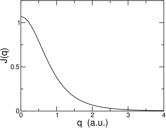
Figure 1: DHF Compton profiles of He, $J(q)$, computed using the well-tempered basis setbasis-mat , and the universal basis setbasis-malli , as a function of the momentum transfer $q$. Profiles obtained using the two basis functions are virtually indistinguishable.

III.2 Ne

DHF calculations were performed for Ne using: (i) $(14s$, $14p$) well-tempered basis set of Matsuoka and Huzinagabasis-mat , and the (ii) large ($32s$, $29p$) universal basis set of Malli et al.basis-malli . In order to facilitate direct comparison with the experiments, the valence CPs (excluding the contribution from the $1s$ core orbital) obtained from our calculations are presented in table 2. They are also compared to the nonrelativistic HF results of Clementi and Roettihe-hf , classic experiment of Eisenbergerexp-ne-eis , and more recent experiment of Lahmam-Bennani et al.exp-ne-jcp . Additionally, the total Compton profiles of Ne (including the contribution of the $1s$ orbital), computed using both the aforesaid basis sets, are plotted in Fig. 2.

Table 2: Relativistic (DHF) valence Compton profiles of Ne atom computed using various basis functions, compared to the nonrelativistic HF resultshe-hf , and the experimentscp-exp-1 .

$q$(a.u.)	$J(q)$(WT)a	$J(q)$(Uni)b	$J(q)$ (HF)c	$J(q)$(Exp.)d	$J(q)$(Exp.)e
$0.0$	$2.5439$	$2.5452$	$2.548$	$2.582$	$2.602$
$0.1$	$2.5363$	$2.5375$	$2.540$	$2.574$	$2.593$
$0.2$	$2.5128$	$2.5140$	$2.515$	$2.558$	$2.560$
$0.3$	$2.4722$	$2.4731$	$2.475$	$2.519$	$2.506$
$0.4$	$2.4129$	$2.4133$	$2.418$	$2.451$	$2.435$
$0.5$	$2.3342$	$2.3339$	$2.335$	$2.359$	$2.340$
$0.6$	$2.2367$	$2.2357$	$2.236$	$2.249$	$2.235$
$0.7$	$2.1224$	$2.1210$	$2.120$	$2.124$	$2.099$
$0.8$	$1.9947$	$1.9933$	$1.990$	$1.986$	$1.966$
$0.9$	$1.8579$	$1.8568$	$1.855$	$1.839$	$1.826$
$1.0$	$1.7166$	$1.7159$	$1.715$	$1.685$	$1.690$
$1.2$	$1.4360$	$1.4361$	$1.435$	$1.394$	$1.417$
$1.4$	$1.1776$	$1.1780$	$1.171$	$1.140$	$1.171$
$1.6$	$0.9533$	$0.9537$	$0.951$	$0.921$	$0.975$
$1.8$	$0.7663$	$0.7665$	$0.766$	$0.749$	—
$2.0$	$0.6142$	$0.6144$	$0.619$	$0.608$	—
$2.5$	$0.3559$	$0.3558$	$0.355$	$0.355$	—
$3.0$	$0.2125$	$0.2123$	$0.212$	$0.225$	—
$3.5$	$0.1318$	$0.1319$	$0.132$	$0.156$	—
$4.0$	$0.0852$	$0.0853$	$0.085$	$0.102$	—
$5.0$	$0.0397$	$0.0397$	$0.040$	$0.041$	—

^aOur DHF results computed using the well-tempered basis setbasis-mat

^bOur DHF results computed using the universal basis setbasis-malli

^cNonrelativistic HF results from Ref.he-hf

^dExperimental results from Ref.exp-ne-eis
^eExperimental results from Ref.exp-ne-jcp

Upon inspecting table 2 we notice the following trends: (i) profiles computed using two different sets are again in very good agreement with each other, implying that both the basis sets are essentially complete, (ii) our relativistic profiles are in quite good agreement with the nonrelativistic HF profileshe-hf essentially implying that even in Ne, the relativistic effects are quite negligible. As far as comparison with the experiments is concerned, for smaller values of $q$ there is slight disagreement with the theory which progressively disappears as one approaches the large momentum-transfer regime. This suggests that electron-correlation effects possibly play an important role in the small momentum transfer regime.

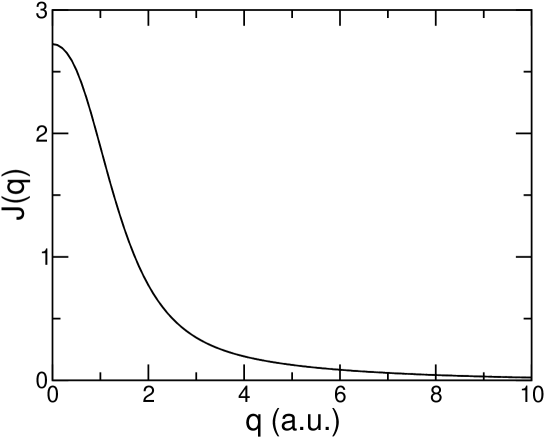
Figure 2: DHF Compton profiles of Ne, $J(q)$, computed using the well-tempered basis setbasis-mat , and the universal basis setbasis-malli , as a function of the momentum transfer $q$. Profiles obtained using the two basis sets are virtually indistinguishable. All numbers are in atomic units.

Finally we examine the individual orbital CPs of the Ne atom in Fig. 3. The maximum contribution to the total CP for small values of momentum transfer comes from the $2s$ orbital, while in the same region, the smallest contribution comes from the $1s$ core orbital. The orbital CP of the $2s$ orbital varies rapidly with respect to $q$ and becomes quite small for $q\geq 2$ a.u. On the other hand the orbital profile of the $1s$ orbital shows the least dispersion with respect to $q$, and has the largest magnitude in the large $q$ region, as compared to other orbital profiles. The behavior of the $2p_{1/2}/2p_{3/2}$ orbital profiles is intermediate as compared to the two extremes of $1s$ and $2s$ profiles. These profiles have lesser magnitude compared to the $2s$ profile for $q\approx 0$, while they vary more rapidly with respect to $q$, when compared to the $1s$ profile. Another pointer to the insignificance of the relativistic effects for Ne is the fact that the difference in the values of the $2p_{1/2}$ and $2p_{3/2}$ is quite small for all values of $q$.

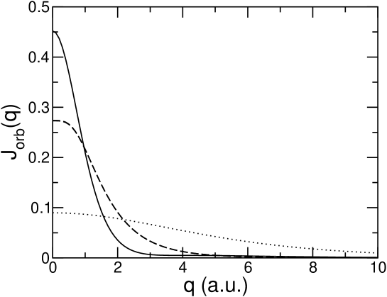
Figure 3: Orbital Compton profiles of Ne for $2s$ (solid line), $2p_{3/2}$/$2p_{1/2}$ (dashed line), and $1s$ (dotted line), plotted with respect to $q.$ Compton profiles of $2p_{1/2}$ and $2p_{3/2}$ orbitals are virtually indistinguishable. These profiles were computed using the universal basis setbasis-malli .

III.3 Ar

Next, we discuss our calculated Compton profiles of Ar. The DHF calculations on Ar atom were performed using the following two basis sets: (i) smaller $(16s$,$16p$) well-tempered basis set of Matsuoka and Huzinagabasis-mat , and the (ii) large ($32s$,$29p)$ universal basis set of Malli et al.basis-malli . Calculated total CPs of Ar, for a selected number of $q$ values in the range $0$ a.u.$\leq q\leq 15$ a.u., are presented in table 3. The same table also contains the nonrelativistic HF results of Clementi and Roettihe-hf , numerical-orbital-based DHF results of Mendelsohn et al.rel-com-prof , and the experimental results of Eisenberger and Reedcp-exp-1 .

Table 3: Our relativistic (DHF) total Compton profiles of Ar atom computed using various basis sets, compared to the relativistic results of other authorsrel-com-prof , the nonrelativistic HF resultshe-hf , and the experimentscp-exp-1 .

$q$(a.u.)	$J(q)$(WT)a	$J(q)$(Uni)b	$J(q)$(DHF)c	$J(q)$(HF)d	$J(q)$(Exp.)e
$0.0$	$5.0471$	$5.0543$	$5.05$	$5.052$	$5.058\pm 0.7\%$
$0.1$	$5.0229$	$5.0302$	$5.03$	$5.028$	$5.022$
$0.2$	$4.9473$	$4.9539$	$4.95$	$4.950$	$4.917$
$0.3$	$4.8130$	$4.8171$	—	$4.812$	$4.749$
$0.4$	$4.6143$	$4.6144$	$4.61$	$4.608$	$4.526$
$0.5$	$4.3528$	$4.3487$	—	$4.369$	$4.259$
$0.6$	$4.0395$	$4.0324$	$4.03$	$4.028$	$3.960$
$0.7$	$3.6928$	$3.6854$	—	$3.690$	$3.643$
$0.8$	$3.3343$	$3.3288$	—	$3.328$	$3.319$
$0.9$	$2.9842$	$2.9814$	—	$2.982$	$3.000$
$1.0$	$2.6576$	$2.6573$	$2.66$	$2.658$	$2.697\pm 1\%$
$1.2$	$2.1071$	$2.1088$	—	$2.108$	$2.164$
$1.4$	$1.7011$	$1.7022$	—	$1.701$	$1.753$
$1.6$	$1.4163$	$1.4166$	—	$1.417$	$1.461$
$1.8$	$1.2198$	$1.2197$	—	$1.221$	$1.264$
$2.0$	$1.0825$	$1.0824$	$1.08$	$1.084$	$1.129$
$2.5$	$0.8728$	$0.8727$	—	$0.873$	$0.904$
$3.0$	$0.7360$	$0.7360$	—	$0.736$	$0.744$
$3.5$	$0.6216$	$0.6217$	—	$0.621$	$0.634$
$4.0$	$0.5207$	$0.5208$	$0.521$	$0.520$	$0.534\pm 2.5\%$
$7.0$	$0.1773$	$0.1774$	—	$0.177$	$0.181$
$8.0$	$0.1300$	$0.1300$	—	$0.130$	$0.137$
$9.0$	$0.0981$	$0.0981$	—	$0.098$	$0.104$
$10.0$	$0.0758$	$0.0757$	$0.076$	$0.075$	$0.078\pm 10\%$
$15.0$	$0.0254$	$0.0254$	—	$0.025$	$0.025$

^aour DHF results computed using the well-tempered basis setbasis-mat

^bour DHF results computed using the universal basis setbasis-malli

^cDHF results of Mendelsohn et al.rel-com-prof based upon finite-difference calculations

^dNonrelativistic HF results from Ref.he-hf

^eExperimental results from Ref.cp-exp-1

Additionally, in Figs. 4 and 5, respectively, we present our total and orbital CPs of Ar plotted as a function of the momentum transfer $q$. From Ar onwards, CP results of Mendelsohn et al. rel-com-prof exist, which were computed from the DHF orbitals obtained from finite-difference-based calculations. If our calculated CPs are correct, they should be in good agreements with those of Mendelsohn et al.rel-com-prof . Therefore, it is indeed heartening for us to note that our CP results computed with the universal basis setbasis-malli are in perfect agreement with those of Mendelsohn et al.rel-com-prof to the decimal places, and for the $q$ points, reported by them. As a matter of fact even our CPs obtained using the smaller well-tempered basis setbasis-mat , disagree with those of Mendelsohn et al.rel-com-prof by very small amounts. Thus, this gives us confidence about the essential correctness of our approach.

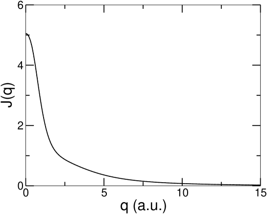
Figure 4: DHF Compton profiles of Ar, $J(q)$, computed using the well-tempered basis setbasis-mat , and the universal basis setbasis-malli , as a function of the momentum transfer $q$. Profiles obtained using the two basis sets can be seen to differ slightly for $q\approx 0$.

When compared to the experiments, for $q=0$, our value of CP of $5.054$ computed with universal basis set, is in excellent agreement with the experimental value of $5.058$cp-exp-1 . For $0.1$a.u.$\leq q\leq$$0.8$a.u. our results begin to overestimate the experimental ones slightly. For $q\geq$$0.9$a.u., however, our theoretical results underestimate the experimental results by small amounts. The nonrelativistic HF resultshe-hf also exhibit the same pattern with respect to the experimental results. Upon comparing our CPs to the nonrelativistic HF CPshe-hf , we notice that the two sets of values differ slightly for smaller values of $q$. However, the difference between the two begins to become insignificant as we approach larger values of $q$, suggesting that the relativistic effects will be most prominent for $q\approx 0$.

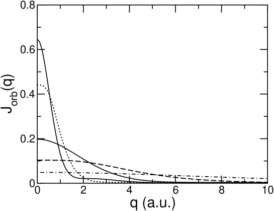
Figure 5: Orbital Compton profiles of Ar, plotted as functions of the momentum transfer $q$. In the decreasing order of the value of $J_{\mbox{orb}}(q=0)$, the profiles correspond to $3s$, $3p_{3/2}/3p_{1/2}$, $2s$, $2p_{3/2}/2p_{1/2}$, and $1s$ orbitals. Note that for all the cases, profiles of $p_{3/2}$ and $p_{1/2}$ orbitals are virtually identical. These profiles were computed using the universal basis setbasis-malli .

Finally we examine the contributions of the individual orbitals to the atomic CP in Fig. 5, which presents the orbital profiles of all the orbitals of Ar. We observe the following trends: (i) $3s$ profile has the maximum value at $q=0$, followed by $3p_{3/2}/3p_{1/2}$ profiles. The minimum value at $q=0$ corresponds to the $1s$ profile. (ii) Profiles of outer orbitals vary more rapidly with $q$, as compared to the inner ones. In other words, profile flattening occurs as one moves inwards from the valence to the core orbitals. (iii) Again no significant fine-structure splitting is observed, in that the profiles of $np_{3/2}$ and $np_{1/2}$ orbitals differed from each other by small amounts, pointing to the smallness of relativistic effects.

III.4 Kr

Now, we discuss our DHF results of Compton profile of Kr. The DHF calculations on Kr atom were performed using the following two basis sets: (i) smaller $(20s$,$15p$, $9d$) basis set of Koga et al.tate-1 , and the (ii) large ($32s$, $29p,$ $20d$) universal basis set of Malli et al.basis-malli . Calculated total CPs of Kr, for $0$ a.u.$\leq q\leq 30$ a.u., are presented in table 4, which also contains the nonrelativistic HF profiles computed by Clementi and Roettihe-hf , DHF profiles calculated by Mendelsohn et al.rel-com-prof , and the experimental results of Eisenberger and Reedcp-exp-1 .

Table 4: Our results on total profiles of Kr computed using the smaller basis set of Koga, Tatewaki and Matsuoka (KTM)tate-1 , and the universal basis setbasis-malli . Relativistic results of other authorsrel-com-prof , nonrelativistic HF resultshe-hf , and the experimental resultscp-exp-1 are also presented for comparison.

$q$(a.u.)	$J(q)$(KTM)a	$J(q)$(Uni)b	$J(q)$(DHF)c	$J(q)$(HF)d	$J(q)$(Exp.)e
$0.0$	$7.1788$	$7.1871$	$7.19$	$7.228$	$7.205$
$0.1$	$7.1470.$	$7.1548$	$7.15$	$7.194$	$7.152$
$0.2$	$7.0452$	$7.0505$	$7.05$	$7.085$	$7.022$
$0.3$	$6.8588$	$6.8595$	—	$6.888$	$6.767$
$0.4$	$6.5780$	$6.5735$	$6.57$	$6.595$	$6.459$
$0.5$	$6.2087$	$6.2010$	—	$6.216$	$6.098$
$0.6$	$5.7744$	$5.7670$	$5.77$	$5.776$	$5.701$
$0.7$	$5.3093$	$5.3053$	—	$5.309$	$5.289$
$0.8$	$4.8485$	$4.8486$	—	$4.848$	$4.880$
$0.9$	$4.4197$	$4.4225$	—	$4.420$	$4.491$
$1.0$	$4.0395$	$4.0429$	$4.04$	$4.039$	$4.133$
$1.2$	$3.4425$	$3.4432$	—	$3.441$	$3.540$
$1.4$	$3.0368$	$3.0353$	—	$3.037$	$3.122$
$1.6$	$2.7662$	$2.7650$	—	$2.769$	$2.850$
$1.8$	$2.5787$	$2.5785$	—	$2.583$	$2.670$
$2.0$	$2.4362$	$2.4364$	$2.44$	$2.441$	$2.533$
$2.5$	$2.1425$	$2.1428$	—	$2.144$	$2.219$
$3.0$	$1.8571$	$1.8572$	—	$1.857$	$1.898$
$3.5$	$1.5784$	$1.5782$	—	$1.578$	$1.597$
$4.0$	$1.3257$	$1.3255$	$1.33$	$1.326$	$1.338$
$5.0$	$0.9333$	$0.9335$	—	$0.934$	$0.937$
$6.0$	$0.6773$	$0.6773$	$0.677$	$0.678$	$0.683$
$7.0$	$0.5118$	$0.5118$	—	$0.512$	$0.522$
$8.0$	$0.4001$	$0.4001$	—	$0.400$	$0.399$
$9.0$	$0.3205$	$0.3205$	—	$0.319$	$0.316$
$10.0$	$0.2608$	$0.2608$	$0.261$	$0.259$	$0.254$
$15.0$	$0.1062$	$0.1062$	—	$0.104$	$0.095$
$20.0$	$0.0506$	$0.0506$	—	$0.049$	$0.044$
$25.0$	$0.0271$	$0.0271$	$0.027$	$0.026$	$0.022$
$30.0$	$0.0157$	$0.0157$	—	$0.015$	$0.009$

^aDHF results computed using the basis set of Koga, Tatewaki and Matsuokatate-1 .

^bDHF results computed using the universal basis setbasis-malli

^cDHF results of Mendelsohn et al.rel-com-prof based upon finite-difference calculations

^dNonrelativistic HF results from Ref.he-hf

^eExperimental results from Ref.cp-exp-1

In Figs. 6 and 7, respectively, our total and orbital CPs of Kr, are plotted as a function of the momentum transfer $q$. Upon comparing our CPs of Kr obtained using two basis sets we note that: (i) for small values of $q$, the values obtained using the smaller basis set of Koga et al.tate-1 are slightly smaller than the ones obtained using the universal basis set, and (ii) for large values of $q$, the results obtained using the two basis sets are in excellent agreement with each other. Next, we compare our calculated CPs with those computed by Mendelsohn et al.rel-com-prof using the numerical orbitals obtained in their DHF calculations. From table 4 it is obvious that, for the all the $q$ values for which Mendelsohn et al.rel-com-prof reported their CPs, our profiles obtained using the universal basis setbasis-malli , are in exact agreement with their results. As a matter of fact, the agreement between the results of Mendelsohn et al.rel-com-prof , and our results computed using the smaller basis set of Koga et al.tate-1 , is also excellent.

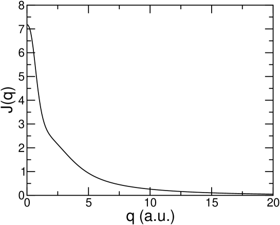
Figure 6: DHF Compton profile of Kr, $J(q)$, computed using the universal basis setbasis-malli , plotted as a function of the momentum transfer $q$.

Upon comparing our results to experimental ones, we see that our universal basis set value of $J(q=0)=7.187$, is in excellent agreement with the experimental value of $7.205$cp-exp-1 . For other values of momentum transfer in the range $0.1$ a.u.$\leq q\leq$$1.0$ a.u., although the agreement between our results and the experiments is slightly worse, yet our results are closer to the experimental value as compared to the nonrelativistic HF resultshe-hf . For higher values of momentum transfer, our DHF results are fairly close to the HF results suggesting that in the region of large $q$, relativistic effects are unimportant. Thus, we conclude that from Kr onwards, relativistic effects make their presence felt in the small $q$ region.

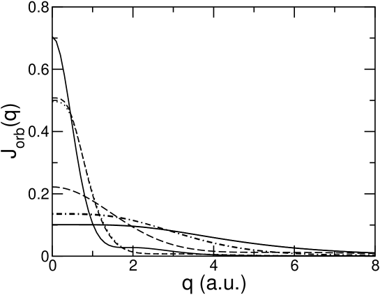
Figure 7: Orbital Compton profiles of Kr for $4s$, $4p_{3/2}$, $4p_{1/2}$, $3s$, $3p_{3/2}$/$3p_{1/2}$, and $3d_{5/2}$/$3d_{3/2}$ orbitals in the order of decreasing values at $q=0$. For small $q$ values, the differences between the $4p_{3/2}$ and $4p_{1/2}$ profiles are visible. These profiles were computed using the universal basis setbasis-malli .

Finally, we investigate the orbital CPs of Kr in Fig. 7, which presents the plots of the profiles of outer orbitals starting from $3d_{3/2}$ to $4p_{3/2}$. As far as the general trends of the orbital profiles are concerned, they are similar to what we observed for the cases of Ne and Ar, except for one important aspect. Unlike the Ne and Ar, for Kr for the first time we begin to observe the fine structure splitting in the orbital profiles of $4p_{3/2}$ and $4p_{1/2}$ orbitals in the low $q$ region, as is obvious from Fig. 7. For example, for $q=0$, corresponding values are $J_{4p_{3/2}}=0.508$, and $J_{4p_{1/2}}=0.496$, amounting to a difference of $\approx 2\%$. This is in complete agreement with our earlier observation that the relativistic effects make significant contributions to the CPs of Kr in the small $q$ region.

III.5 Xe

In this section, we discuss our results on the relativistic Compton profiles of Xe. The DHF calculations on Xe atom were performed using the following two basis sets: (i) smaller $(22s$,$18p$, $12d$) basis set of Koga et al.tate-1 , and the (ii) large ($32s$, $29p,$ $20d$) universal basis set of Malli et al.basis-malli . Total CPs of Xe, for selected values of momentum transfer in the range $0$ a.u.$\leq q\leq 100$ a.u., are presented in table 5. For the sake of comparison, the same table also contains DHF, and the nonrelativistic HF, profiles calculated by Mendelsohn et al.rel-com-prof . Here, we are unable to compare our results with the experiments, because, to the best of our knowledge, no experimental measurements of the CPs of Xe exist.

Table 5: Total CPs of Xe computed using the smaller basis set of Koga, Tatewaki and Matsuoka (KTM)tate-1 , and the universal basis setbasis-malli . Relativistic results of other authorsrel-com-prof , and nonrelativistic HF resultsrel-com-prof are also presented for comparison.

$q$(a.u.)	$J(q)$(KTM)a	$J(q)$(Uni)b	$J(q)$(DHF)c	$J(q)$(HF)d
$0.0$	$9.722$	$9.737$	$9.74$	$9.88$
$0.1$	$9.673$	$6.687$	$9.69$	$9.82$
$0.2$	$9.515$	$9.523$	$9.52$	$9.65$
$0.4$	$8.784$	$8.775$	$8.78$	$8.85$
$0.6$	$7.597$	$7.587$	$7.59$	$7.62$
$1.0$	$5.448$	$5.451$	$5.45$	$5.46$
$1.5$	$4.293$	$4.292$	$4.29$	$4.31$
$2.0$	$3.678$	$3.678$	$3.68$	$3.69$
$4.0$	$1.707$	$1.707$	$1.71$	$1.72$
$6.0$	$1.060$	$1.061$	$1.06$	$1.06$
$10.0$	$0.5150$	$0.5150$	$0.515$	$0.515$
$25.0$	$0.0660$	$0.0662$	$0.066$	$0.064$
$50.0$	$0.0088$	$0.0088$	$0.0088$	$0.0076$
$100.0$	$0.00067$	$0.0067$	$0.00068$	$0.00043$

^aour DHF results computed using the basis set of Koga, Tatewaki and Matsuokatate-1 .

^bour DHF results computed using the universal basis setbasis-malli

^cDHF results of Mendelsohn et al.rel-com-prof based upon finite-difference calculations

^dNonrelativistic HF results reported in Ref.rel-com-prof

Additionally, in Figs. 8 and 9, respectively, we present the plots of our total and orbital CPs of Xe. Upon comparing our total CPs obtained using the two basis sets we find that, as before, they disagree for smaller values of $q$, with the CPs obtained using the smaller basis settate-1 being slightly lower than those obtained using the universal basis setbasis-malli . As is obvious from table 5, that for $q\geq 1.5$ a.u., the two sets of basis functions yield virtually identical results. In the same table, when we compare our results to the earlier DHF results of Mendelsohn et al.rel-com-prof , we find that for all the $q$ values, the agreement between our universal basis-set based CPs, and their results, is perfect up to the decimal places reported by them. This again points to the correctness of our calculations.

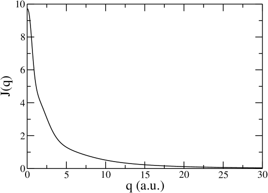
Figure 8: DHF Compton profile of Xe, computed using the universal basis setbasis-malli , and plotted as a function of the momentum transfer $q$.

Upon comparing our DHF results to the nonrelativistic HF results of Mendelsohn et al.rel-com-prof , we find that for smaller values of $q$, the DHF values of CPs are smaller than the HF values, while for large values of $q$, the trend is just the opposite.

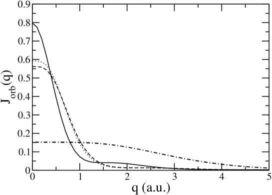
Figure 9: Orbital Compton profiles of Xe for $5s$, $5p_{3/2}$, $5p_{1/2}$, and $4d_{5/2}$/$4d_{3/2}$ orbitals in the order of decreasing values at $q=0$. For small $q$ values, the differences between the $5p_{3/2}$ and $5p_{1/2}$ profiles are quite significant. These profiles were computed using the universal basis setbasis-malli

Finally, upon examining the orbital profiles presented in Fig. 9, we observe further evidence of the importance of relativistic effects in Xe. As is obvious from the figure, the fine-structure splitting between the orbitals profiles of $5p_{3/2}$ and $5p_{1/2}$ orbitals is larger as compared to $4p_{3/2}/4p_{1/2}$ splitting in Kr, and persists for a longer range of $q$ values. For smaller values of $q$, $J_{5p_{3/2}}(q)>J_{5p_{1/2}}(q)$, while for large $q$ values, opposite is the case. For $q=0,$ $J_{5p_{3/2}}=0.592$, while $J_{5p_{1/2}}=0.562$, which amounts to a difference of $\approx 5\%$.

III.6 Rn

As far as atomic Rn is concerned, to the best of our knowledge, no prior experimental studies of its Compton profiles exist. However, Biggs et al.rel-comp-prof-2 did perform DHF calculations of this atom, using a finite difference approach, with which we compare our results later on in this section. Our DHF calculations on Rn atom were performed using the following two basis sets: (i) smaller $(25s$,$21p$, $15d$, $10f$) basis set of Koga et al.tate-2 , and the (ii) large ($32s$, $29p,$ $20d$, $15f$) universal basis set of Malli et al.basis-malli . Total CPs of Rn, for selected values of momentum transfer in the range $0$ a.u.$\leq q\leq 100$ a.u., are presented in table 6.

Table 6: Total CPs of Rn computed using the smaller basis set of Koga, Tatewaki and Matsuoka (KTM)tate-2 , and the universal basis setbasis-malli , compared to the earlier calculations of Biggs et al. rel-comp-prof-2 .

$q$(a.u.)	$J(q)$(KTM)a	$J(q)$(Uni)b	$J(q)$(DHF)c
$0.0$	$11.8344$	$11.8531$	$11.9$
$0.1$	$11.7850$	$11.8026$	$11.8$
$0.2$	$11.6176$	$11.6306$	$11.6$
$0.4$	$10.8055$	$10.7996$	$10.8$
$0.6$	$9.4877$	$9.4744$	$9.47$
$1.0$	$7.2130$	$7.2130$	$7.21$
$1.6$	$5.8127$	$5.8132$	$5.81$
$2.0$	$5.1530$	$5.1533$	$5.15$
$4.0$	$2.8379$	$2.8381$	$2.84$
$6.0$	$2.0453$	$2.0454$	$2.05$
$10.0$	$0.9804$	$0.9804$	$0.98$
$30.0$	$0.1083$	$0.1083$	$0.11$
$60.0$	$0.0166$	$0.0166$	$0.017$
$100.0$	$0.0037$	$0.0037$	$0.0037$

^aour DHF results computed using the basis set of Koga, Tatewaki and Matsuokatate-2 .

^bour DHF results computed using the universal basis setbasis-malli

^cDHF results of Biggs et al.rel-comp-prof-2 based upon finite-difference calculations

Our results for total and orbital CPs of Rn are plotted in Figs. 10 and 11, respectively. As for other atoms, we find that our total CPs obtained using the two basis sets disagree for smaller values of $q$, with the CPs obtained using the smaller basis set of Koga et al.tate-2 being slightly smaller than those obtained using the universal basis setbasis-malli . From table 6 we deduce that for $q\geq 4.0$ a.u., the two sets of basis functions yield virtually identical values of CPs. In the same table, when we compare our results to the earlier DHF calculations of Biggs et al.rel-comp-prof-2 , we find that for all the $q$ values, the agreement between our universal basis-set based CPs, and their results, is perfect up to the decimal places reported by them.

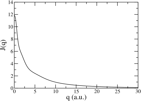
Figure 10: DHF Compton profile of Rn, computed using the universal basis setbasis-malli , and plotted as a function of the momentum transfer $q$.

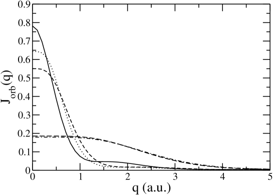
Figure 11: Orbital Compton profiles of Rn for $6s$, $6p_{3/2}$, $6p_{1/2}$, and $5d_{5/2}$/$5d_{3/2}$ orbitals in the order of decreasing values at $q=0$. For small $q$ values, the differences between the $6p_{3/2}$ and $6p_{1/2}$ profiles are quite large. Even the splitting of $5d_{5/2}$ and $5d_{3/2}$ profiles is visible. These profiles were computed using the universal basis setbasis-malli .

Of all the rare gas atoms considered so far, on the intuitive grounds we expect the relativistic effects to be the strongest in Rn. Indeed, this is what we confirm upon investigating the orbital profiles presented in Fig. 11. As is obvious from the figure, the splitting between the orbitals profiles of $6p_{3/2}$ and $6p_{1/2}$ orbitals is quite big, and persists for a large range of $q$ values. Similar to the case of Xe, here also for smaller values of $q$, $J_{6p_{3/2}}(q)>J_{6p_{1/2}}(q)$, while for large $q$ values, opposite is the case. For $q=0,$ $J_{6p_{3/2}}=0.644$, while $J_{6p_{1/2}}=0.551$, amounting to a difference of $\approx 15\%$, which is quite substantial. The fine-structure splitting between the profiles of $5d_{5/2}$ and $5d_{3/2}$ orbitals although is not quite that large, yet it is visible in Fig. 11. At $q=0,$$J_{5d_{5/2}}=0.185$, and $J_{5d_{3/2}}=0.179$, leading to a difference of $\approx 3\%$, which is quite significant for an inner orbital. Thus, we conclude that the relativistic effects are quite substantial in case of Rn, and, therefore, it will be useful if experiments are performed on this system to ascertain this.

III.7 Z dependence of relativistic effects on Compton Profiles

In earlier sections, while discussing relativistic effects on Compton profiles, we noticed that they were most prominent for small momentum transfers. Moreover, one intuitively expects the relativistic effects to increase with increasing atomic number $Z$. In this section our aim is to perform a quantitative investigation of relativistic effects on quantum profiles, as a function of $Z$, for both large and small values of momentum transfer. We noticed that for small momentum transfers, DHF values of $J$ were smaller than their nonrelativistic counterparts, while for large momentum transfer opposite was the case. Therefore, for a given value of momentum transfer $q$, we quantify relativistic effects in terms of $|J(\mbox{DHF})-J(\mbox{HF})|$, which is the magnitude of the difference of relativistic DHF value of the Compton profile ($J(\mbox{DHF})$), and the nonrelativistic HF value of the profile ($J(\mbox{HF})$). We obtain $J(\mbox{HF})$ by using a large value of the velocity of light ($c=10^{4}$ a.u.) in the DHF calculations. We explore the dependence of this quantity on $Z$, for two values of momentum transfer, $q=0$, and $q=Z$ a.u., where the latter value clearly belongs to the large momentum transfer regime. The values of $\ln|J(\mbox{DHF})-J(\mbox{HF})|$ as a function of $\ln Z$, are presented in Fig. 12 for both these values of momentum transfer. From the figure it obvious that, to a very good approximation, the corresponding curves are straight lines, suggesting a power-law dependence of the relativistic effects on $Z$. The slopes of the least-square fit line for $q=0$ is $2.36$ while for $q=Z$, the slope is $1.35$. Of course, these results are based upon data points generated by six values of $Z$ (rare gas series), and consequently can only be treated as suggestive. But the results suggest: (i) super-linear dependence of the relativistic effect on quantum profiles in both momentum transfer regimes, and (ii) stronger influence of relativity in the small momentum transfer regime as compared to the large one. Of course, this exploration can be refined further by separately investigating the $Z$ dependence of these effects on the core and valence profiles. Additionally, this investigation can be extended to a larger number of atoms to obtain a larger set of data points. However, these calculations are beyond the scope of the present work, and will be presented elsewhere.

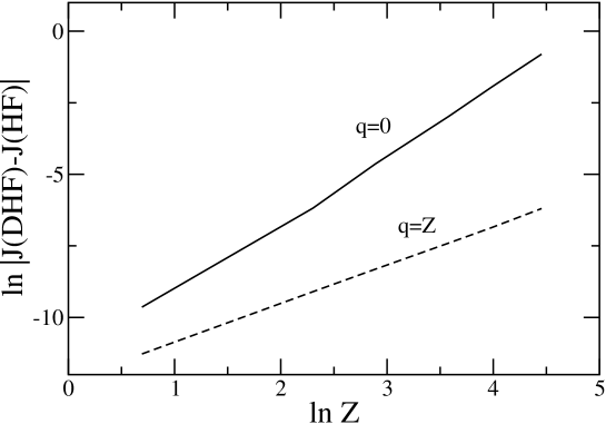
Figure 12: Difference between the relativistic ($J(\mbox{DHF})$), and the nonrelativistic ($J(\mbox{HF})$) Compton profiles plotted, on a logarithmic scale, as a function of the atomic number $Z$. Plots correspond to the momentum transfer values $q=0$, and $q=Z$.

IV Conclusions and Future Directions

In this paper, we presented an approach aimed at computing the relativistic Compton profiles of atoms within the DHF approximation, when the atomic orbitals are represented as linear combinations of kinetically-balanced set of Gaussian functions. The approach was applied to compute the CPs of rare gas atoms ranging from He to Rn, and results were compared to the experimental profiles, and theoretical profiles of other authors, wherever such data was available. Additionally, the influence of size and type of basis set was examined by performing calculations on each atom with two basis sets: (i) a well-known smaller basis set, and (ii) a large universal basis set proposed by Malli et al.basis-malli .

Upon comparing our results with the experiments, we found that for lighter atoms He, Ne, and Ar, the agreement was similar to what one obtains from the nonrelativistic HF calculations, indicating lack of any significant relativistic effects for these atoms. For Kr, we noticed that for smaller momentum transfer values, DHF results were in better agreement with the experiments, as compared to the HF results. For heavier atoms, Xe and Rn, unfortunately no experimental data is available. Yet another quantitative indicator of the importance of relativistic effects is the fine-structure splitting of the profiles, i.e., the difference in the profiles of $np_{1/2}/np_{3/2}$ etc., which will have identical profiles in nonrelativistic calculations. We found that this splitting becomes larger with the increasing atomic number of the atom, thus justifying a relativistic treatment of the problem for heavy atoms. Additionally, by comparing our results with the nonrelativistic HF results we found that the relativistic effects are most prominent in the region of small momentum transfer, while at large momentum transfer, their contribution is much smaller.

In the literature, we were able to locate prior theoretical calculation of relativistic CPs of atoms only from one group, namely the DHF calculations of Mendelsohn et al.rel-com-prof and Biggs et al.rel-comp-prof-2 , performed on Ar, Kr, Xe, and Rn, employing a finite-difference based approach. The CPs computed by themrel-com-prof ; rel-comp-prof-2 for these atoms were found to be in perfect agreement with our results computed using the universal basis set. This testifies to the correctness of our approach, and suggests that by using a large basis set, it is possible to reach the accuracy of finite-difference approaches in relativistic calculations, not just on total energiesbasis-malli , but also on expectation values.

Having investigated the influence of the relativistic effects, the next logical step will be to go beyond the mean-field DHF treatment, and incorporate the influence of electron correlations on atomic CPs, within a relativistic framework. Such a treatment can be within a relativistic CI frameworkci-shukla , or can also be performed within a perturbation-theoretic formalism. Work along these lines is currently underway in our group, and the results will be submitted for publication in future.

Appendix A A Derivation of compton profile Matrix Elements over Kinetically Balanced Gaussian Basis Sets

During our discussion here, we use the same notations for various quantities as adopted in section II.Our aim here is to evaluate the closed form expressions for the following two integrals

$$J_{ij}^{L;\kappa}(q)=\frac{1}{2}\int_{q}^{\infty}pg_{\kappa i}^{L}(p)g_{\kappa j}^{L}(p)\,dp$$ (10)

$$J_{ij}^{S;\kappa}(q)=\frac{1}{2}\int_{q}^{\infty}pg_{\kappa i}^{S}(p)g_{\kappa j}^{S}(p)\,dp$$ (11)

which, as explained in section II, are needed to compute the orbital (and total) atomic CPs when the KBGF based numerical formalism is employed to solve the DHF equations. First, we will obtain expressions for $g_{\kappa i}^{L}(p)$ and $g_{\kappa i}^{S}(p)$, the radial Fourier transforms of the large and small component basis functions $g_{\kappa i}^{L}(r)$ and $g_{\kappa i}^{S}(r)$, respectively, defined as

$$g_{\kappa i}^{L}(p)=\frac{4\pi}{(2\pi)^{3/2}}\int_{0}^{\infty}rg_{\kappa i}^{L}(r)j_{l_{A}}(pr)\,dr$$ (12)

$$g_{\kappa i}^{S}(p)=\frac{4\pi}{(2\pi)^{3/2}}\int_{0}^{\infty}rg_{\kappa i}^{S}(r)j_{l_{B}}(pr)\,dr$$ (13)

where $j_{l_{A}}(pr)/j_{l_{A}}(pr)$ refer to the spherical Bessel functions corresponding to the orbital angular momentum $l_{A}/l_{B}$ of the large/small component. The spherical Bessel function is related to the Bessel function by the well-known relation

$$j_{\nu}(x)=\sqrt{\frac{\pi}{2x}}J_{\nu+1/2}(x),$$ (14)

where $J_{\nu}(x)$ is the Bessel function.

A.1 Derivation for the Large Component

First , we obtain and expression for $g_{\kappa i}^{L}(p)$ by performing the integral involved in Eq. (12). Substituting the expression for $g_{\kappa i}^{L}(r)$ from Eq. (3) in Eq.(12), we obtain

$$g_{\kappa i}^{L}(p) = \frac{4\pi}{(2\pi)^{3/2}}\int_{0}^{\infty}N_{\kappa i}^{L}r^{(n_{\kappa}+1)}e^{-\alpha_{i}r^{2}}j_{l_{A}}(pr)\,dr$$ (15)

$$= \frac{N_{\kappa i}^{L}}{\sqrt{p}}\int_{0}^{\infty}N_{\kappa i}^{L}r^{(n_{\kappa}+1/2)}e^{-\alpha_{i}r^{2}}J_{l_{A}+1/2}(pr)\,dr$$

where in the last step, we have used Eq. (14). Next, on using the relation $n_{\kappa}=l_{A}+1$, and the definite integralabram+steg

$$\int_{0}^{\infty}x^{\nu+1}e^{-\alpha r^{2}}J_{\nu}(\beta x)\,dx=\frac{\beta^{\nu}}{(2\alpha)^{\nu+1}}e^{-\beta^{2}/4\alpha}[Re(\alpha)>0,Re(\nu)>0],$$ (16)

the Eq.(15) simplifies to

$$g_{\kappa i}^{L}(p)=N_{\kappa i}^{L}\frac{p^{l_{A}}}{(2\alpha_{i})^{l_{A}+3/2}}e^{-p^{2}/4\alpha_{i}}.$$ (17)

On substituting the above result in Eq.(10), one obtains

$$J_{ij}^{L;\kappa}(q)=\frac{1}{2}\int_{q}^{\infty}(N_{\kappa i}^{L})(N_{\kappa j}^{L})\frac{p^{2l_{A}+1}}{(4\alpha_{i}\alpha_{j})^{l_{A}+3/2}}e^{-p^{2}/4\alpha_{ij}}\,dp$$

where $\alpha_{ij}=\frac{\alpha_{i}\alpha_{j}}{\alpha_{i}+\alpha_{j}}$. Next, on making the change of variable $t=\frac{p^{2}}{4\alpha_{ij}}$ in the integral above, leading to the lower limit $q_{t}=\frac{q^{2}}{4\alpha_{ij}}$, we obtain

$$J_{ij}^{L;\kappa}(q) = \frac{(N_{\kappa i}^{L})(N_{\kappa j}^{L})}{4}\frac{(4\alpha_{ij})^{l_{A}+1}}{(4\alpha_{i}\alpha_{j})^{l_{A}+3/2}}\int_{q_{t}}^{\infty}t^{l_{A}}e^{-t}\,dt,$$

leading to the final expression

$$J_{ij}^{L;\kappa}(q)=\frac{(N_{\kappa i}^{L})(N_{\kappa j}^{L})}{4}\frac{(4\alpha_{ij})^{l_{A}+1}}{(4\alpha_{i}\alpha_{j})^{l_{A}+3/2}}\Gamma(l_{A}+1,q_{t}),$$ (18)

where $\Gamma(l_{A}+1,q_{t})$ is the incomplete gamma function. Since, $l_{A}$ is a non-negative integer, the incomplete gamma function can be easily computed using the seriesabram+steg ,

$$\Gamma(l_{A}+1,q_{t})=(l_{A})!e^{-q_{t}}\sum_{m=0}^{l_{A}}\frac{{q_{t}}^{m}}{m!}.$$ (19)

We note that our general result for $J_{ij}^{L;\kappa}(q)$ in Eq. (18) leads to the same formulas as reported by Naon et al.naon for the atomic CP matrix elements for s- and p-type Gaussian orbitals, for the nonrelativistic case.

A.2 Derivation for the small component

Noting that the explicit form of the small component basis function $g_{\kappa i}^{S}(r)$ (cf. Eq. (4)) is

$$g_{\kappa i}^{S}(r)=N_{\kappa i}^{S}N_{\kappa i}^{L}\left[(n_{\kappa}+\kappa)r^{n_{\kappa}-1}e^{-\alpha_{i}r^{2}}-2\alpha_{i}r^{n_{\kappa}+1}e^{-\alpha_{i}r^{2}}\right].$$

On substituting the above in Eq.(13), the Fourier transform of the small component basis function becomes

$$g_{\kappa i}^{S}(p)=\frac{N_{\kappa i}^{S}N_{\kappa i}^{L}}{\sqrt{p}}\int_{0}^{\infty}\left[(n_{\kappa}+\kappa)r^{(n_{\kappa}-1/2)}-2\alpha_{i}r^{(n_{\kappa}+3/2)}\right]e^{-\alpha_{i}r^{2}}J_{l_{B}+1/2}(pr)\,dr$$ (20)

As before, we seek a relation between $n_{\kappa}$ and $l_{B}$, which is summarized in table 7. Here, the two cases have to be dealt separately since, the relations are different for the two possibilities.

Table 7: Relationship between quantum numbers $\kappa$, $n_{\kappa}$, and $l_{B}$, for relativistic atomic orbitals.

$\kappa$	$n_{\kappa}$	$l_{B}$
$-(j+\frac{1}{2})$	$-\kappa$	$j+\frac{1}{2}=-\kappa$
$(j+\frac{1}{2})$	$\kappa+1$	$j-\frac{1}{2}=\kappa-1$

Case (i) $\kappa=-(j+1/2)$ :

From table 7, it is easy to see that for this case, $n_{\kappa}=l_{B}=-\kappa$. The integral in Eq.(20) becomes

$$g_{\kappa i}^{S}(p) = \frac{N_{\kappa i}^{S}N_{\kappa i}^{L}}{\sqrt{p}}\int_{0}^{\infty}(-2\alpha_{i})r^{(n_{\kappa}+3/2)}e^{-\alpha_{i}r^{2}}J_{n_{\kappa}+1/2}(pr)\,dr,$$ (21)

$$= -N_{\kappa i}^{S}N_{\kappa i}^{L}\frac{p^{n_{\kappa}}}{(2\alpha_{i})^{(n_{\kappa}+1/2)}}e^{-p^{2}/4\alpha_{i}}.$$

Case (ii) $\kappa=(j+1/2)$ :

For this case, $l_{B}=n_{\kappa}-2=\kappa-1$, which upon substitution in Eq.(20) yields

$$g_{\kappa i}^{S}(p) = \frac{N_{\kappa i}^{S}N_{\kappa i}^{L}}{\sqrt{p}}\int_{0}^{\infty}\left[(2n_{\kappa}-1)r^{(n_{\kappa}-1/2)}-2\alpha_{i}r^{(n_{\kappa}+3/2)}\right]e^{-\alpha_{i}r^{2}}J_{n_{\kappa}-3/2}(pr)\,dr.$$ (22)

Next we use the resultabram+steg

$$\int_{0}^{\infty}x^{\mu}e^{-\alpha x^{2}}J_{\nu}(\beta x)\,dx = \frac{\beta^{\nu}\Gamma\left(\frac{\nu}{2}+\frac{\mu}{2}+\frac{1}{2}\right)}{2^{\nu+1}\alpha^{\frac{1}{2}(\mu+\nu+1)}\Gamma(\nu+1)}\Phi\left(\frac{\nu+\mu+1}{2},\nu+1,-\frac{\beta^{2}}{4\alpha}\right)$$ (23)

$$\mbox{for }Re(\alpha)>0,Re(\mu+\nu)>-1,$$

where $\Phi(a,b,z)$ is the confluent hypergeometric function, in Eq. (22), and after some simplifications obtain

$$g_{\kappa i}^{S}(p) = \frac{N_{\kappa i}^{S}N_{\kappa i}^{L}}{\sqrt{p}}\frac{p^{(n_{\kappa}-3/2)}}{2^{(n_{\kappa}-3/2)}{\alpha_{i}}^{(n_{\kappa}-1/2)}}\left[\left(n_{\kappa}-\frac{1}{2}\right)\Phi\left(n_{\kappa}-\frac{1}{2},n_{\kappa}-\frac{1}{2},-\frac{p^{2}}{4\alpha_{i}}\right)\right.$$ (24)

$$\left.-\left(n_{\kappa}-\frac{1}{2}\right)\Phi\left(n_{\kappa}+\frac{1}{2},n_{\kappa}-\frac{1}{2},-\frac{p^{2}}{4\alpha_{i}}\right)\right]$$

Next, we use the following two identities involving the confluent hypergeometric functionsabram+steg

$$a\Phi(a+1,b,z)=(z+2a-b)\Phi(a,b,z)+(b-a)\Phi(a-1,b,z),$$ (25)

and

$$\Phi(a,a,z)=e^{z},$$ (26)

to obtain the following simple expression from Eq. (24)

$$g_{\kappa i}^{S}(p)=N_{\kappa i}^{S}N_{\kappa i}^{L}\frac{p^{n_{\kappa}}}{(2\alpha_{i})^{(n_{\kappa}+1/2)}}e^{-p^{2}/4\alpha_{i}}.$$ (27)

Comparing the results of two cases (21) and (27), we find that they only differ by a sign, and hence when substituted in the expression for $J_{ij}^{S;\kappa}(q)$ in Eq.(11) yield the same result

$$J_{ij}^{S;\kappa}(q)=\frac{1}{2}\int_{q}^{\infty}(N_{\kappa i}^{S})(N_{\kappa j}^{S})(N_{\kappa i}^{L})(N_{\kappa j}^{L})\frac{p^{2n_{\kappa}+1}}{(4\alpha_{i}\alpha_{j})^{n_{\kappa}+1/2}}e^{-p^{2}/4\alpha_{ij}}\,dp,$$

where $\alpha_{ij}=\frac{\alpha_{i}\alpha_{j}}{\alpha_{i}+\alpha_{j}}$ . The above integral can be evaluated in exactly the same way as was done before for the large component (cf. 18), to yield the final expression for the Compton profile matrix element

$$J_{ij}^{S;\kappa}(q)=\frac{(N_{\kappa i}^{S})(N_{\kappa j}^{S})(N_{\kappa}^{L}i)(N_{\kappa j}^{L})}{4}\frac{(4\alpha_{ij})^{l_{A}+2}}{(4\alpha_{i}\alpha_{j})^{l_{A}+3/2}}\Gamma(l_{A}+2,q_{t}),$$ (28)

where $q_{t}=\frac{q^{2}}{4\alpha_{ij}}$, and the incomplete gamma function is defined in Eq. (19). Finally, the large and small components of the CP of an orbital can be computed in terms of these matrix elements, as

$$J_{n\kappa}^{L}(q)=\sum_{i,j}C_{\kappa i}^{L}C_{\kappa j}^{L}J_{ij}^{L;\kappa},$$ (29)

$$J_{n\kappa}^{S}(q)=\sum_{i,j}C_{\kappa i}^{S}C_{\kappa j}^{S}J_{ij}^{S;\kappa}.$$ (30)

It is these formulas derived here which have been numerically implemented in our computer program COMPTONcp-program aimed at calculating relativistic atomic CPs.

References

- (1) For a review see I. P. Grant, in Methods in Computational Chemistry, edited by S. Wilson (Plenum, New York, 1988), Vol. 12, p. 1.
- (2) Y. K. Kim, Phys. Rev. 154, 17 (1967).
- (3) T. Kagawa, Phys. Rev. A 12, 2245 (1975).
- (4) Y. Ishikawa, R.C. Binning, and K.M. Sando, Chem. Phys. Lett. 101, 111 (1983)
- (5) K.G. Dyall, I.P. Grant and S. Wilson, J. Phys. B 17, 493 (1984).
- (6) R. E. Stanton and S. Havriliak, J. Chem. Phys. 81, 1910 (1984).
- (7) A. K. Mohanty and E. Clementi, Chem. Phys. Lett. 157, 348 (1989); ibid., J. Chem. Phys. 93, 1829 (1990).
- (8) O. Visser, L. Visscher, P.J.C. Aerts, and W.C. Nieuwpoort, Theor. Chim. Acta 81, 405 (1992); O. Matsuoka, L. Pisani, and E. Clementi, Chem. Phys. Lett. 20, 13 (1993) ; F. A. Parpia and A.K. Mohanty, Phys. Rev. A 52, 962 (1995); A.K. Mohanty and F.A. Parpia, Phys. Rev. A 54, 2863 (1996) .
- (9) A. Shukla, M. Dolg, H.-J. Flad, A. Banerjee, and A. K. Mohanty, Phys. Rev. A 55, 3433 (1997).
- (10) L. Visscher, O. Visser, P. J. C. Aerts, H. Merenga, and W. C. Nieuwpoort, Comput. Phys. Commun. 81, 120 (1994); Y. Watanabe and O. Matsuoka, J. Chem. Phys. 116, 9585 (2002).
- (11) For a review see, Compton Scattering, edited by B. G. Williams, (McGraw Hill, Great Britain, 1977).
- (12) A. Shukla, M. Dolg, P. Fulde and, H. Stoll, Phys. Rev. B 57, 1471 (1998).
- (13) For a review of inelastic photon scattering from the inner-shell electrons, see, P. P. Kane, Phys. Rep. 218, 67 (1992).
- (14) L. B. Mendelsohn, F. Biggs, and J. B. Mann, Chem. Phys. Letts. 26, 521 (1974).
- (15) F. Biggs, L. B. Mendelsohn, and J. B. Mann, At. Data. Nuc. Data Tables 16, 201 (1975).
- (16) R. Ribberfors, Phys. Rev. B 12, 2067 (1975).
- (17) P. Holm, Phys. Rev. A 37, 3706 (1988).
- (18) P. M. Bergstrom, Jr., T. Surić, K. Pisk, R. H. Pratt, Phys. Rev. A 48, 1134 (1993).
- (19) P. Eisenberger and P. M. Platzman, Phys. Rev. A 2, 415 (1970).
- (20) Computer program COMPTON, P. Jaiswal and A. Shukla, in preparation.
- (21) A.K. Mohanty and E. Clementi, in Modern Techniques in Computational Chemistry, edited by E. Clementi (ESCOM, Leiden, 1989), p. 169; also see the work of Mohanty and Clementi in Ref. cal-at-dhf .
- (22) G. L. Malli, A. B. F. Da Silva, and Y. Ishikawa, Phys. Rev. A 47, 143 (1993).
- (23) O. Matsuoka and S. Huzinaga, Chem. Phys. Letts. 140, 567 (1987).
- (24) E. Clemenit and C. Roetti, At. Data Nucl. Data Tables 14, 177 (1974).
- (25) P. Eisenberger and W.A. Reed, Phys. Rev. A 5, 2085 (1972).
- (26) P. Eisenberger, Phys. Rev. A 5, 628 (1972).
- (27) A. Lahmam-Bennani, A. Duguet, and M. Rouault, J. Chem. Phys. 78, 1838 (1983).
- (28) T. Koga, H. Tatewaki and O. Matsuoka, J. Chem. Phys. 115, 3561 (2001).
- (29) T. Koga, H. Tatewaki and O. Matsuoka, J. Chem. Phys. 119, 1279 (2003).
- (30) M. Abramowitz and I. A. Stegun, eds., Handbook of Mathematical Functions with Formulas, Graphs, and Mathematical Tables (Dover, New York, 1965).
- (31) M. Naon, M. Cornille, M. Roux, J. Phys. B 4, 1593 (1971).