Microcanonical and canonical approach
to traffic flow

Abstract

A system of identical cars on a single-lane road is treated as a microcanonical and canonical ensemble. Behaviour of the cars is characterized by the probability of car velocity as a function of distance and velocity of the car ahead. The calculations a performed on a discrete 1D lattice with discrete car velocities.

Probability of total velocity of a group of cars as a function of density is calculated in microcanonical approach. For a canonical ensemble, fluctuations of car density as a function of total velocity is found. Phase transitions between free and jammed flow for large deceleration rate of cars and formation of queues of cars with the same velocity for low deceleration rate are described.

1 Introduction

Traffic flow of a system of identical cars on a single-lane road has been intensively studied in recent decade using dynamical or kinetic description of car behaviour. [1,2] The models used were continuous (fluid dynamical models), car-following models [3], or discrete particle hopping models related to cellular automaton models with stochastic behaviour [4]. In this paper we develop an approach to this problem based not on equations of motion or master equations describing the system of cars, but in the spirit of statistical mechanics where:

– Each state of the system is occupied by equal probability and physical properties of the system are analyzed calculating number of states for some fixed physical quantities in the microcanonical description. Logarithm of number of states is called entropy.

– In the canonical approach the probability of states depends on their energy, and the logarithm of number of all states (weighted by their probabilities, with negative sign and divided by temperature). is called free energy.

Here we assume that the probability of the car velocity is a function of the velocity, and the distance of the car ahead, while all the distances between two cars are equally probable, i.e., from the point of view of statistical mechanics, a combination of the canonical and microcanonical approach is used. Despite of that, further it is denoted as a microcanonical one.

The car distances are treated purely microcanonically only in the first part of the paper. In the second one, the density of a group of cars is not fixed, but it is a part of larger microcanonical ensemble with fixed number of cars. Here the probability of distances between two cars depends on the length of the group, and the distances are treated in the same way as velocities, i.e., canonically.

In our approach no assumptions about the drivers’ behaviour and car properties are necessary – the probability of the car velocity can be measured experimentally, nevertheless, in this paper it is derived from a simple model behaviour of cars.

In statistical physics the term microcanonical ensemble means, as a rule, an isolated system, in which some physical quantities are conserved and thus are constant. In our microcanonical approach the system is not assumed to be isolated, but only such states of the system, or a subsystem, are taken into account, for which some quantities remain constant. In a system of cars this may be, e.g., sum of the velocities of all cars or their density. The subsystem is influenced by a boundary condition – the distribution of velocities of the car ahead of the investigated group.

In the approach of Mahnke et al. [5] the group of cars is represented by a grandcanonical ensemble, number of cars in which is not fixed, and its chemical potential is a function of parameters of a master equation. In our approach the thermodynamics of the system of cars is systematically derived starting from the microcanonical approach. The properties of a canonical ensemble are deduced from the known entropy of a subsystem together with a reservoir. When the size of the cluster of cars inside the reservoir is changed, the derivative of entropy represents a pressure exerted by reservoir of cars on the group, instead of chemical potential in the above-mentioned work.

In the last years we could observe a revival of the microcanonical approach to the problems of statistical mechanics [6–10]. One of the reasons for it was that the region where the entropy of a finite system is convex, instead of the standard concave shape of it, was identified as a point or line in the phase space where the first-order phase transition in corresponding infinite system takes place. As the number of observed cars in normal traffic is not too large, the techniques developed in statistical physics for small systems are convenient in this case. The term “phase transition” in this paper is used in the sense of the above-cited works.

2 Model and method

The cars are further represented by dimensionless points moving on a discrete one-dimensional lattice, and are characterized by 2 quantities: discrete velocity $v_{i}$ in the interval $\langle 0,v_{\rm max}\rangle$ and a discrete coordinate (site number) $x_{i}\in\langle 1,L\rangle$. $v_{\rm max}$ is the maximum velocity given by the construction of the car and $L$ is the length of the observed group (subsystem) of cars. The coordinate of each car is measured with respect to the last car of the group. Its coordinate is always 0, i.e., the origin of the coordinate system is fixed to it. As the length of the group is $L$, the coordinate of the last car of the group ahead is $L$. Number of cars in the group is $N$. (The lattice constant is related to the car length). Car velocities and coordinates acquire only integer values. Car velocities are random, described by a probability distribution peaked around an optimal velocity $v_{\rm opt}$, which is further chosen as 90% of maximal safe velocity $v_{\rm m}$. The maximal safe velocity is determined from the requirement that two neighbouring cars, which start to decelerate at the same time with the same deceleration rate $a$, would stop without crash. Moreover, $v_{\rm m}$ must not be greater than the maximum possible velocity of the car $v_{\rm max}$, i.e., for every car

$$v_{\rm opt}(v_{2},x_{1,2})=0.9v_{\rm m}(v_{2},x_{1,2}),$$

$$v_{\rm m}(v_{2},x_{1,2})=\left\{{\begin{array}[]{*{20}l}\sqrt{2ax_{1,2}+v_{2}^{2}}&{\rm if}\ v_{\rm m}\leq v_{\rm max}\\ v_{\rm max}&{\rm if}\ v_{\rm m}>v_{\rm max}\\ \end{array}}\right.$$ (3)

where $x_{1,2}$ and $v_{2}$ are the distance (headway) and velocity of the car ahead, respectively. The reaction time of the driver in (1) is assumed to be equal to zero, nevertheless, it can be easily generalized for nonzero reaction times with only a small impact on our final results. (This problem is discussed in more detail in [11]. As we use only integer values of velocities, the nearest integer value to $v_{\rm opt}$ from (1) is taken for the actual optimal velocity in our calculations.

The way of driving of the observed drivers is characterized by distribution of probabilities of car velocities around the optimal velocity. Here we use an extremely simple distribution, in which the probability of optimal velocity is $p_{0}$, the probabilities of the velocities $v_{\rm opt}\pm 1$ are $p_{1}$, while the probability of the car to have any other permitted velocity is $p_{2}$. The sum of all probabilities for each car is equal to 1. The parameters $p_{0},p_{1}$ and $p_{2}$ are the same for every car, and the distribution depends on the headway only by means of the value of optimal velocity.

3 Microcanonical description

In the microcanonical approach only such groups of $N$ cars, which length is $L$ and sum of their velocities is $V$, are studied. These groups of cars are influenced only by the velocity distribution of the car ahead of them with coordinate $L$. The probability distribution of each car is given by the rule above as a function of headway and the velocity of the car ahead, while the distances between them are arbitrary and limited only by the length of the group.

The probability that the sum of velocities of $N$ cars in a group of length $L$ is $V$ multiplied by the number of their configurations on $L$ sites, is further denoted as $W(V,L)$ and called density of states. It can be calculated recurrently

$$W_{1}(V_{1},L_{1};v_{2})=p(V_{1};L_{1},v_{2})$$

$$\vdots$$

$$W_{i}(V_{i},L_{i};v_{i+1})=\sum_{v_{i},x_{i,i+1}}W_{i-1}(V_{i}-v_{i},L_{i}-x_{i,i+1};v_{i})p(v_{i};x_{i,i+1},v_{i+1})$$

$$\hbox{for }i=2,N-1$$

$$\vdots$$ (4)

$$W_{N}(V,L;v_{N+1})=$$

$$\qquad{}=\sum_{v_{N},x_{N,N+1}}W_{N-1}(V-v_{N},L-x_{N,N+1};v_{N})p(v_{N};x_{N,N+1},v_{N+1})$$

$$W(V,L)=\sum_{v_{N+1}}W_{N}(V,L;v_{N+1})p(v_{N+1})$$

where $0\leq v_{j}\leq v_{\rm max}$, $0\leq V_{j}\leq jv_{\rm max}$, $j\leq x_{j,j+1},L_{j}\leq L-j$. $p(v_{N+1})$ in the last line of (2) is the velocity probability of the last car of a large group ahead of the studied group with the same car density. This large group will be further called reservoir.

Density of states in the reservoir of length $L_{\rm r}$, number of cars $N_{\rm r}$, with the density $\displaystyle{N_{\rm r}\over L_{\rm r}}={N\over L}$, and fixed velocity of the last car $v_{N+1}$ is

$$W_{\rm r}(v_{N+1},L_{\rm r})=\sum_{v_{N+2},\dots,v_{N+N_{\rm r}}\atop x_{N+1,N+2},\dots,x_{N+N_{\rm r},N+N_{\rm r}+1}}\prod_{i=N+1}^{N+N_{\rm r}}p_{i}(v_{i};x_{i,i+1},v_{i+1})\delta_{L_{\rm r},\sum x_{i,i+1}}$$ (5)

It depends, in principle, on the velocity of the first car of the reservoir, but numerical calculations show that for large $N_{\rm r}$ this dependence is negligible. The probability $p(v_{N+1})$ is the normalized density of states $W$

$$p(v_{N+1})=W_{\rm r}(v_{N+1},L_{\rm r})/\sum_{v_{N+1}}W_{\rm r}(v_{N+1},L_{\rm r})$$ (6)

The quantity $W(V,L)$ in (3) expresses the probability that the sum of velocities of the cars in the group is $V$ as well as the number of possible configurations of occupation of $L$ sites by $N$ cars. As mentioned above, it is, in fact, a product of probability $P$ and number of configurations $\Omega$

$$W(V,L)={W(V,L)\over\sum_{V}W(V,L)}\cdot\sum_{V}W(V,L)\equiv P(V,L)\cdot\Omega(L).$$ (7)

As for the fixed length of the subsystem, $\Omega(L)$ is constant, only the normalized probability $P(V,L)$ is be presented in Results.

In the microcanonical approach only subsystems of cars with the constant density, the same as is the mean density of the whole system, are studied. To take into account also the density fluctuations, it is more convenient to use the canonical description with variable density of the subsystem due to its variable length.

4 Canonical description

In canonical approach the length of the subsystem varies, only the length of the whole system, subsystem + reservoir is fixed. The number of cars in the subsystem and in the reservoir remains constant, so the density of cars varies with varying length of the groups. Our canonical description differs from the grandcanonical approach of Mahnke et al. [5] where the density of the subsystem changes due to exchange of cars between the subsystem and reservoir.

In statistical mechanics the properties of a reservoir are usually not calculated, only the values of derivatives of its entropy (logarithm of number of states) with respect to the quantities, which are fixed in the whole system, are assumed to be known. They are, e.g., temperature, chemical potential, etc. Similarly, in our canonical description of the system of cars, a pressure of reservoir exerted on the subsystem could be introduced. Nevertheless, this quantity cannot be directly measured, and it would depend on the velocity of the last car of the reservoir, so we prefer a direct calculation of number of states of a large enough reservoir for given velocity of the last car and length of the reservoir.

The length of the system $L_{\rm s}$ is the sum of the length of the subsystem and reservoir $X+L_{\rm r}$. The number of cars in the subsystem and reservoir are fixed and denoted as $N$ and $N_{\rm r}$, respectively. If $X\ll L_{\rm r}$ and $N\ll N_{\rm r}$, the properties of the subsystem does not depend on velocity of the first car in the reservoir.

Density of states of the reservoir at given velocity of the last car is calculated according to (5). Density of states of the whole system at given total velocity of the subsystem $V$ and its length $X$ can be obtained by the same way as in the microcanonical case, only in the last term in (3) – the probability of the velocity of the last reservoir car $p(v_{n+1})$ – is replaced by the density of states of the reservoir. Last line of (3) now reads

$$W(V,X)=\sum_{v_{n+1}}W_{n}(V,X;v_{n+1})W_{\rm r}(v_{n+1},L_{\rm s}-X).$$ (8)

The mean density of the subsystem $N/\langle X\rangle$ is equal to the density of the whole system $(N+N_{\rm r})/L_{\rm s}$.

The main difference between the microcanonical and canonical treatment is that in the first case only number of states of the subsystem is calculated while in the latter case the properties of the subsystem are given by the number of states of the whole system. In the microcanonical approach the reservoir is used only for calculation of boundary condition – probability distribution of the last car of the subsystem. It is summed over all car velocities and positions. In the canonical system the summation is performed only over velocity degrees of freedom as the velocity even of the whole system is not conserved.

5 Results and discussion

The velocities and positions of cars are described by discrete variables in our model. Changing the values of its parameters, we can observe two different types of behaviour. In the first one, for high deceleration rate $a$ and low densities, the system behaves like continuous; in the density of states the underlying discrete structure of velocities is not seen. At small $a$ and high densities, total velocities of the system, which are integer multiples of number of particles, are more probable then the others. This regime reminds a ferromagnetic Potts model where the total magnetization of the system points in many different directions of the space.

In all our calculations, car velocity acquires 21 values $v_{i}=i,\ i=0,20$. The probability of a car to move with a velocity $v_{i}$ depends on the velocity and distance of the car ahead by means of optimal velocity $v_{\rm opt}(v,x)$. It acquires 3 values $p(v_{\rm opt})=p_{0}$, $p(v_{\rm opt}\pm 1)=p_{1}$, $p(v_{i})=p_{2}$ for all other $v_{i}$. Only two of these parameters are independent as the probability is normalized: $\sum_{i=0}^{20}p(v_{i})=1$. In the present calculations $p_{1}$ is fixed to 0.3, and $p_{2}$ was chosen for the only free parameter of the velocity distribution. The position of a car with respect to the first one may be an integer between 0, and $L-1$ if the site is not occupied by another car. In the free-flow regime the deceleration rate $a$ in (1) is put equal to 4.0, in the jammed regime, where the discreteness of the velocity plays role, $a=0.5$.

The main result of our calculations are density of states $W(V,X)$ in the canonical case and probability of the total velocity, $P(V,X)$, of the subsystem as a function of the subsystem length at fixed number of cars for microcanonical ensemble. They are plotted in 3D graphs.

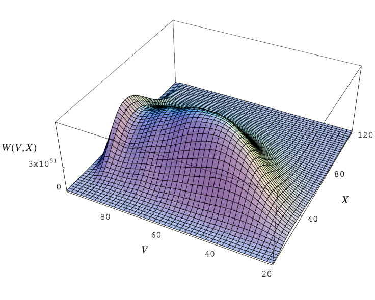
Figure 1: Density of states of a canonical ensemble of 5 cars as a function of its total velocity $V$ and length $X$ for $a=4.0$, $p_{2}=0.03$, and mean length $\langle X\rangle=50$, i.e., mean density $\rho=0.1$.

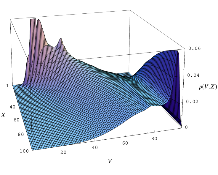
Figure 2: Probability of the total velocity of a microcanonical ensemble of 5 cars as a function of its total velocity $V$ and length $X$ for $a=4.0$, $p_{2}=0.025$. The density of the system varies from 0.05 to 1.

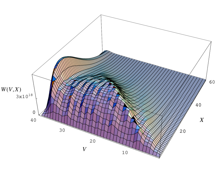
Figure 3: Density of states of a canonical ensemble of 2 cars as a function of its total velocity $V$ and length $X$ for $a=4.0$, $p_{2}=0.03$ and mean length $\langle X\rangle=25$, i.e., mean density $\rho=0.1$.

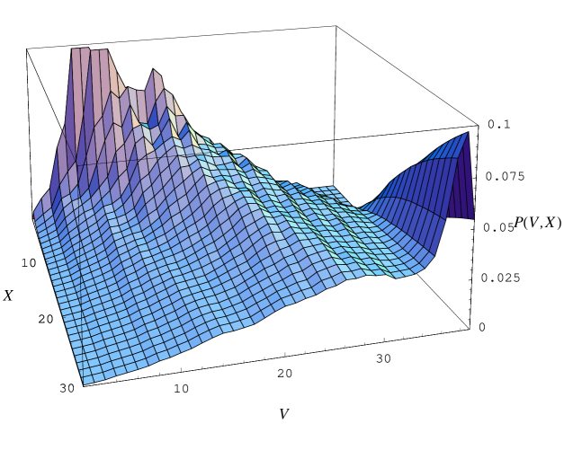
Figure 4: Probability of the total velocity of a microcanonical ensemble of 2 cars as a function of its total velocity $V$ and length $X$ for $a=4.0$, $p_{2}=0.03$. The density of the system varies from 0.05 to 1.

In the free-flow regime with $a=4$, the shape of density of states $W$, in canonical ensemble, depends on the parameter $p_{2}$. For $p=0$, practically all the cars have their velocity close to the optimal one with the most probable density at the value of the mean density of the system. For large probabilities of the small and large velocities, $p_{2}>0.05$, the density of states is represented by a broad peak with maximum of less than one half of the optimal velocity, and the cars also in this regime become jammed. In Fig. 1 an intermediate case is shown with a narrow free-flow peak and a broad peak of jammed cars. The plot represents distribution of density of states for 5 cars creating a group of length $X$ with total velocity $V$. The group is a part of a large system of cars with fixed total length with density 0.1, i.e., the mean length of the group of 5 cars is 50.

As expected, the velocity of jammed cars is lower that of those moving freely. Most probable total velocity of the jammed group is about 2/3 of the total velocity of freely moved group, which density is about 20% smaller. As the car flow in both groups is different, they cannot coexist in a finite system in steady state. Both peaks represent two states of the system of cars with very low transition rate between them, which is expressed by the depth of the minimum between them. Two neighbouring fluctuation can live long only if they have the same mean velocity per particle. On the other hand, as the plot has only one maximum for constant $V$, the probability of such fluctuations is low.

In the microcanonical case the length of the subsystem determines the density of cars not only in the subsystem but also in the whole system together with reservoir. The length of the group is fixed, and there are no length fluctuation of it. The probability of total velocity of 5 cars for various density of the whole system is shown in Fig. 2. The plot is viewed from opposite direction than in Fig. 1. For length of the group $X=50$, it corresponds to the canonical system of length $L=50$ (Fig. 1), which is equal to the mean length of the group. While in Fig. 1 the plot for small $X$ represents behaviour of dense fluctuations, in Fig. 2 the whole system together with reservoir is dense. It can be seen that for $X=5$ the most probable state is when all cars have velocity 4.

For high densities the most probable state has a small velocity, for low densities the most probable velocity is the optimal one. The first-order phase transition occurs when the height of low and high velocity peak is equal; in Fig. 2, it is at $X=38.$ It should be stressed that the phase transition introduced in this paper is not the phase transition exactly in thermodynamic sense as the system of cars is finite. In this system cannot coexist large groups of cars in different phases, i.e., with different velocities. Then the transition from a local maximum to absolute maximum of probability is very improbable, and a strong hysteresis occurs in the system, observed also experimentally [12].

In Fig. 3 and 4 the same plots, but for 2 cars only, are shown. The free-flow peak is more pronounced in Fig. 3. It can be explained by the fact that also in a jammed 5-car group, 2 cars may move fast for a short time. The average length of the group in canonical ensemble is now 20. For two-car groups the discreteness of model velocities in the density of states and probability of velocity is manifested. For 5 or more cars, these quantities are smoothed, and the model can simulate to some extent a real traffic.

The discreteness is conspicuous for low braking ability of cars and high densities. For $a=0.5$ and $N/\langle X\rangle=0.2$ it can be seen in Fig. 5. In this case, especially for fluctuation with high densities, the cars have tendency to form queues with the same velocity of each car.

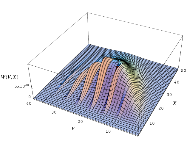
Figure 5: Density of states of a canonical ensemble of 5 cars as a function of its total velocity $V$ and length $X$ for $a=0.5$, $p_{2}=0.01$ and mean length $\langle X\rangle=25$, i.e., mean density $\rho=0.1$.

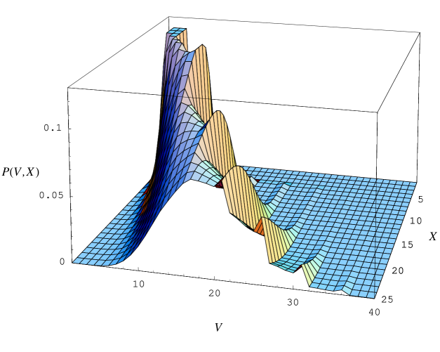
Figure 6: Probability the of total velocity of a microcanonical ensemble of 5 cars as a function of its total velocity $V$ and length $X$ for $a=0.5$, $p_{2}=0.01$. The density of the system varies from 0.2 to 1.

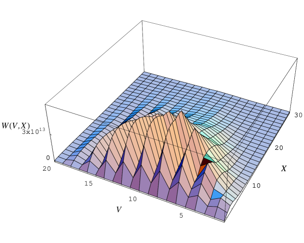
Figure 7: Density of states of a canonical ensemble of 2 cars as a function of its total velocity $V$ and length $X$ for $a=0.5$, $p_{2}=0.01$ and mean length $\langle X\rangle=10$, i.e., mean density $\rho=0.2$.

Figure 8: Probability of the total velocity of a microcanonical ensemble of 2 cars as a function of its total velocity $V$ and length $X$ for $a=0.5$, $p_{2}=0.01$. The density of the system varies from 0.066 to 1.

For low densities $(X>25)$ and small velocities, these queues are dissolved. The microcanonical picture of the system is in Fig. 6. Now probability distributions have a number of local maxima. Each of them can become an absolute maximum for some values of $X$. Large velocity maxima are absolute maxima for low densities of cars.

For a system of 2 cars with the same parameters, the density of states and probabilities are in Figs. 7, 8. Here the queues of cars with equal velocity consist of 2 cars, and the probability of total velocity has peaks at even values of $V$.

For small deceleration rates $a$, the velocity probability consists of number of peaks representing phases with different total velocities and first-order phase transitions between them. The difference between these velocities can be taken as an order parameter in the concrete phase transitions. With increasing $a$ the valley between two probability peaks is disappearing, the order parameter becomes zero, and a second-order phase transitions takes place. For large $a$ (Fig. 1, 2) the distance between the peaks remains always large. Changing the parameter $p_{2}$, one of the peaks disappears, but merging of two peaks into one, i.e. the second-order phase transition, is never observed.

In conclusion, the microcanonical and canonical decription of a system of cars was developed. The only input into the theory is the probability of car velocity as a function distance and velocity of the car ahead. According to standard procedure in statistical mechanics, all other missing information are replaced by the principle of maximum entropy of the system. From these assumptions pressure-density diagram of the system can be derived, but here, only directly observable quantities as density of states and probability of the total velocity of a group of cars were presented.

We acknowledge support from VEGA grant No. 2/6071/2006.

References

- [1] D. E. Wolf, M. Schreckenberg, and A. Bachem (Eds.), Traffic and Granular Flow, World Scientific, 1996; D. Helbing, H.J. Herrmann, M. Schreckenberg, D.E. Wolf (Eds.), Traffic and GranularFlow 99, Springer, Berlin, 2000; M. Fukui, Y. Sugiyama, M. Schreckenberg, D.E. Wolf (Eds.), Traffic and GranularFlow 01, Springer, Heidelberg, 2003; S.P. Hoogendoorn, P.H.L. Bovy, M. Schreckenberg, D.E. Wolf (Eds.), Springer, Heidelberg, 2005.
- [2] D. Helbing, Rev. Mod. Phys., 73, 1067 (2001).
- [3] R. Herman, K. Gardels, Sci. Am. 209, 35 (1963)
- [4] K. Nagel and M. Schreckenberg, J. Phys. I (France) 2, 2221 (1992).
- [5] R. Mahnke, J. Hinkel, J. Kaupužs, and H. Weber, Thermodynamics of traffic flow, cond-mat/0606509 (2006).
- [6] D. H. E. Gross, Microcanonical thermodynamics: Phase transitions in “small” systems, Lecture Notes in Physics, 66, World Scientific, Singapore, (2001).
- [7] R. J. Creswick, Physical Review E, 52, 5735 (1995)
- [8] D.H.E. Gross, Geometric Foundation of Thermo-Statistics, Phase Transitions, Second Law of Thermodynamics, but without Thermodynamic Limit, cond-mat/0201235 (2002)
- [9] M. Kastner, M. Promberger, and A. Hüller, J. Stat. Phys. 99, 1251 (2000).
- [10] H. Behringer, On the structure of the entropy surface of microcanonical systems, Mensch und Buch Verlag, Berlin, (2004).
- [11] R. Jiang, M.B. Hu, B. Jia, R.L. Wang, and Q.S. Wu, Eur. Phys. J. B 54, 267 (2006).
- [12] D. Chowdhury, L. Santen and A. Schadschneider, Physics Reports 329, 199 (2000).