Dissipative Boussinesq equations

Abstract

The classical theory of water waves is based on the theory of inviscid flows. However it is important to include viscous effects in some applications. Two models are proposed to add dissipative effects in the context of the Boussinesq equations, which include the effects of weak dispersion and nonlinearity in a shallow water framework. The dissipative Boussinesq equations are then integrated numerically.

1 Introduction

Boussinesq equations are widely used in coastal and ocean engineering. One example among others is tsunami wave modelling. These equations can also be used to model tidal oscillations. Of course, these types of wave motion are perfectly described by the Navier-Stokes equations, but currently it is impossible to solve fully three-dimensional (3D) models in any significant domain. Thus, approximate models such as the Boussinesq equations must be used.

The years 1871 and 1872 were particularly important in the development of the Boussinesq equations. It is in 1871 that Valentin Joseph Boussinesq received the Poncelet prize from the Academy of Sciences for his work. In the Volumes 72 and 73 of the “Comptes Rendus Hebdomadaires des Séances de l’Académie des Sciences”, which cover respectively the six-month periods January–June 1871 and July–December 1871, there are several contributions of Boussinesq. On June 19, 1871, Boussinesq presents the now famous note on the solitary wave entitled “Théorie de l’intumescence liquide appelée onde solitaire ou de translation, se propageant dans un canal rectangulaire” (72, pp. 755–759), which will be extended later in the note entitled “Théorie générale des mouvements qui sont propagés dans un canal rectangulaire horizontal” (73, pp. 256–260). Saint-Venant presents a couple of notes of Boussinesq entitled “Sur le mouvement permanent varié de l’eau dans les tuyaux de conduite et dans les canaux découverts” (73, pp. 34–38 and pp. 101–105). Saint-Venant himself publishes a couple of notes entitled “Théorie du mouvement non permanent des eaux, avec application aux crues des rivières et à l’introduction des marées dans leur lit” (73, pp. 147–154 and pp. 237–240). All these notes deal with shallow-water theory. On November 13, 1871, Boussinesq submits a paper entitled “Théorie des ondes et des remous qui se propagent le long d’un canal rectangulaire horizontal, en communiquant au liquide contenu dans ce canal des vitesses sensiblement pareilles de la surface au fond”, which will be published in 1872 in the Journal de Mathématiques Pures et Appliquées (17, pp. 55–108).

Boussinesq (1871, 1872) included dispersive effects for the first time in the Saint-Venant equations (de Saint-Venant, 1871). One should mention that Boussinesq’s derivation was restricted to $1+1$ dimensions ($x$ and $t$) and a horizontal bottom. Boussinesq equations contain more physics than the Saint-Venant equations but at the same time they are more complicated from the mathematical and numerical point of views. These equations possess a hyperbolic structure (the same as in the nonlinear shallow-water equations) combined with high-order derivatives to model wave dispersion. There have been a lot of further developments of these equations like in Peregrine (1967); Nwogu (1993); Wei et al. (1995); Madsen and Schaffer (1998).

Let us outline the physical assumptions. The Boussinesq equations are intended to describe the irrotational motion of an incompressible homogeneous inviscid fluid in the long wave limit. The goal of this type of modelling is to reduce 3D problems to two-dimensional (2D) ones. This is done by assuming a polynomial (usually linear) vertical distribution of the flow field, while taking into account non-hydrostatic effects. This is the principal physical difference with the nonlinear shallow-water (NSW) equations.

There are a lot of forms of the Boussinesq equations. This diversity is due to different possibilities in the choice of the velocity variable. In most cases one chooses the velocity at an arbitrary water level or the depth-averaged velocity vector. The resulting model performance is highly sensitive to linear dispersion properties. The right choice of the velocity variable can significantly improve the propagation of moderately long waves. A good review is given by Kirby (2003). There is another technique used by Bona et al. (2002). Formally, one can transform higher-order terms by invoking lower-order asymptotic relations. It provides an elegant way to improve the properties of the linear dispersion relation and it gives a quite general mathematical framework to study these systems.

The main purpose of this article is to include dissipative effects in the Boussinesq equations. It is well-known that the effect of viscosity on free oscillatory waves on deep water was studied by Lamb (1932). What is less known is that Boussinesq himself studied this effect as well. Boussinesq wrote three related papers in 1895 in the “Comptes Rendus Hebdomadaires des Séances de l’Académie des Sciences”: (i) “Sur l’extinction graduelle de la houle de mer aux grandes distances de son lieu de production : formation des équations du problème” (120, pp. 1381-1386), (ii) “Lois de l’extinction de la houle en haute mer” (121, pp. 15-20), (iii) “Sur la manière dont se régularise au loin, en s’y réduisant à une houle simple, toute agitation confuse mais périodique des flots” (121, pp. 85-88). It should be pointed out that the famous treatise on hydrodynamics by Lamb has six editions. The paragraphs on wave damping are not present in the first edition (1879) while they are present in the third edition (1906). The authors did not have access to the second edition (1895), so it is possible that Boussinesq and Lamb published similar results at the same time. Indeed Lamb derived the decay rate of the linear wave amplitude in two different ways: in paragraph 348 of the sixth edition by a dissipation calculation (this is also what Boussinesq (1895) did) and in paragraph 349 by a direct calculation based on the linearized Navier-Stokes equations. Let $\alpha$ denote the wave amplitude, $\nu$ the kinematic viscosity of the fluid and $k$ the wavenumber of the decaying wave. Boussinesq (see Eq. (12) in Boussinesq (1895)) and Lamb both showed that

$$\frac{\partial\alpha}{\partial t}=-2\nu k^{2}\alpha.$$ (1)

Equation (1) leads to the classical law for viscous decay of waves of amplitude $\alpha$, namely $\alpha\sim\exp(-2\nu k^{2}t)$ (see Eq. (13) in Boussinesq (1895) after a few calculations).

In the present paper, we use two different models for dissipation and derive corresponding systems of long-wave equations. There are several methods to derive the Boussinesq equations but the resulting equations are not the same. So one expects the solutions to be different. We will investigate numerically whether corresponding solutions remain close or not.

One may ask why dissipation is needed in Boussinesq equations. First of all, real world liquids are viscous. This physical effect is “translated” in the language of partial differential equations by dissipative terms (e.g. the Laplacian in the Navier-Stokes equations). So, it is natural to have analogous terms in the long wave limit. In other words, a non-dissipative model means that there is no energy loss, which is not pertinent from a physical point of view, since any flow is accompanied by energy dissipation.

Let us mention an earlier numerical and experimental study by Bona et al. (1981). They pointed out the importance of dissipative effects for accurate long wave modelling. In the “Résumé” section one can read

[…] it was found that the inclusion of a dissipative term was much more important than the inclusion of the nonlinear term, although the inclusion of the nonlinear term was undoubtedly beneficial in describing the observations […].

The complexity of the mathematical equations due to the inclusion of this term is negligible compared to the benefit of a better physical description.

Let us consider the incompressible Navier-Stokes (N-S) equations for a Newtonian fluid:

$$\nabla\cdot\mathbf{u}^{*} =0,$$

$$\frac{\partial\mathbf{u}^{*}}{\partial t^{*}}+\mathbf{u}^{*}\cdot\nabla\mathbf{u}^{*} =-\frac{\nabla p^{*}}{\rho}+\nu\Delta\mathbf{u}^{*}+\frac{\mathbf{F}^{*}}{\rho},$$

where $\mathbf{u}^{*}(x,y,z,t)=(u^{*},v^{*},w^{*})(x^{*},y^{*},z^{*},t^{*})$ is the fluid velocity vector, $p^{*}$ the pressure, $\mathbf{F}^{*}$ the body force vector, $\rho$ the constant fluid density and $\nu$ the kinematic viscosity.

Switching to dimensionless variables by introducing a characteristic velocity $U$, a characteristic length $L$ and a characteristic pressure $\rho U^{2}$, neglecting body forces in this discussion, the N-S equations become

$$\nabla\cdot\mathbf{u} =0,$$

$$\frac{\partial\mathbf{u}}{\partial t}+\mathbf{u}\cdot\nabla\mathbf{u} =-\nabla p+\frac{1}{Re}\Delta\mathbf{u},$$

where $Re$ is the well-known dimensionless parameter known as the Reynolds number and defined as

$$Re=\frac{F_{inertia}}{F_{viscous}}=\frac{UL}{\nu}.$$

From a physical point of view the Reynolds number is a measure of the relative importance of inertial forces compared to viscous effects. For typical tsunami propagation applications the characteristic particle velocity $U$ is about $5$ cm/s and the characteristic wave amplitude, which we use here as characteristic length scale, is about $1$ m. The kinematic viscosity $\nu$ depends on the temperature but its order of magnitude for water is 10^-6 m²/s. Considering that as the tsunami approaches the coast both the particle velocity and the wave amplitude increase, one can write that the corresponding Reynolds number is of the order of 10⁵ or 10⁶. This simple estimate clearly shows that the flow is turbulent (as many other flows in nature).

It is a common practice in fluid dynamics (addition of an “eddy viscosity” into the governing equations for Large Eddy Simulations) to ignore the small-scale vortices when one is only interested in large-scale motion. It can significantly simplify computational and modelling aspects. So the inclusion of dissipation can be viewed as the simplest way to take into account the turbulence.

There are several authors (Tuck, 1974; Longuet-Higgins, 1992; Spivak et al., 2002; Skandrani et al., 1996; Dias et al., 2007; Ruvinsky et al., 1991) who included dissipation due to viscosity in potential flow solutions and there are also authors (Kennedy et al., 2000; Zelt, 1991; Heitner and Housner, 1970) who already included in Boussinesq models ad-hoc dissipative terms into momentum conservation equations in order to model wave breaking. Modelling this effect is not the primary goal of the present paper, since the flow is no longer irrotational after wave breaking. Strictly speaking the Boussinesq equations can no longer be valid at this stage. Nevertheless scientists and engineers continue to use these equations even to model the run-up on the beach. In our approach a suitable choice of the eddy viscosity, which is a function of both space and time, can model wave breaking at least as well as in the articles cited above.

2 Derivation of the Boussinesq equations

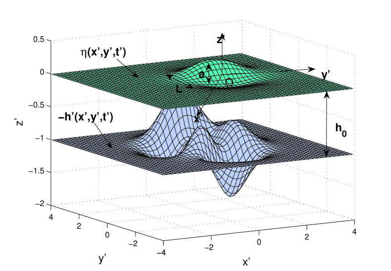
Figure 1: Sketch of the fluid domain

In order to derive the Boussinesq equations, we begin with the full water-wave problem. A Cartesian coordinate system $(x^{\prime},y^{\prime},z^{\prime})$ is used, with the $x^{\prime}-$ and $y^{\prime}-$axis along the still water level and the $z^{\prime}-$ axis pointing vertically upwards. Let $\Omega_{t}$ be the fluid domain in $\mathbb{R}^{3}$ which is occupied by an inviscid and incompressible fluid. The subscript $t$ underlines the fact that the domain varies with time and is not known a priori. The domain $\Omega_{t}$ is bounded below by the seabed $z^{\prime}=-h^{\prime}(x^{\prime},y^{\prime},t^{\prime})$ and above by the free surface $z^{\prime}=\eta^{\prime}(x^{\prime},y^{\prime},t^{\prime})$. In this section we choose the domain $\Omega_{t}$ to be unbounded in the horizontal directions in order to avoid the discussion on lateral boundary conditions. The reason is twofold. First of all, the choice of the boundary value problem (BVP) (e.g. generating and/or absorbing boundary, wall, run-up on a beach) depends on the application under consideration and secondly, the question of the well-posedness of the BVP for the Boussinesq equations is essentially open. Primes stand for dimensional variables. A typical sketch of the domain $\Omega_{t}$ is given in Figure 1. If the flow is assumed to be irrotational one can introduce the velocity potential $\phi^{\prime}$ defined by

$$\vec{u}^{\prime}=\nabla^{\prime}\phi^{\prime},\qquad\nabla^{\prime}\ :=\left(\frac{\partial}{\partial x^{\prime}},\frac{\partial}{\partial y^{\prime}},\frac{\partial}{\partial z^{\prime}}\right)^{T},$$

where $\vec{u}^{\prime}$ denotes the velocity field. Then we write down the following system of equations for potential flow theory in the presence of a free surface:

$$\Delta^{\prime}\phi^{\prime}=0,\qquad(x^{\prime},y^{\prime},z^{\prime})\in\Omega_{t}=\mathbb{R}^{2}\times[-h^{\prime},\eta^{\prime}],$$

$$\phi^{\prime}_{z^{\prime}}=\eta^{\prime}_{t^{\prime}}+\nabla^{\prime}\phi^{\prime}\cdot\nabla^{\prime}\eta^{\prime},\qquad z^{\prime}=\eta^{\prime},$$

$$\phi^{\prime}_{t^{\prime}}+\frac{1}{2}\left|\nabla^{\prime}\phi^{\prime}\right|^{2}+g\eta^{\prime}=0,\qquad z^{\prime}=\eta^{\prime},$$ (2)

$$\phi^{\prime}_{z^{\prime}}+h^{\prime}_{t^{\prime}}+\nabla^{\prime}\phi^{\prime}\cdot\nabla^{\prime}h^{\prime}=0,\qquad z^{\prime}=-h^{\prime},$$

where $g$ denotes the acceleration due to gravity (surface tension effects are usually neglected for long-wave applications). It has been assumed implicitly that the free surface is a graph and that the pressure is constant on the free surface (no forcing). Moreover we assume that the total water depth remains positive, i.e. $\eta^{\prime}+h^{\prime}>0$ (there is no dry zone).

As written, this system of equations does not contain any dissipation. Thus, we complete the free-surface dynamic boundary condition (2) by adding a dissipative term to account for the viscous effects:

$$\phi^{\prime}_{t^{\prime}}+\frac{1}{2}\left|\nabla^{\prime}\phi^{\prime}\right|^{2}+g\eta^{\prime}+D^{\prime}_{\phi^{\prime}}=0,\qquad z^{\prime}=\eta^{\prime}.$$

In this work we investigate two models for the dissipative term $D^{\prime}_{\phi^{\prime}}$. For simplicity, one can choose a constant dissipation model (referred hereafter as Model I) which is often used (e.g. (Jiang et al., 1996)):

$$\mbox{Model I:}\qquad D^{\prime}_{\phi^{\prime}}:=\delta_{1}\phi^{\prime}.$$ (3)

There is a more physically realistic dissipation model which is obtained upon balancing of normal stress on the free surface (e.g. (Ruvinsky et al., 1991; Zhang and Vinals, 1997; Dias et al., 2007)):

$$\mbox{Model II:}\qquad D^{\prime}_{\phi^{\prime}}:=\delta_{2}\phi^{\prime}_{z^{\prime}z^{\prime}}.$$ (4)

The derivation of Boussinesq equations is more transparent when one works with scaled variables. Let us introduce the following independent and dependent non-dimensional variables:

$$x=\frac{x^{\prime}}{\ell},\qquad y=\frac{y^{\prime}}{\ell},\qquad z=\frac{z^{\prime}}{h_{0}},\qquad t=\frac{\sqrt{gh_{0}}}{\ell}t^{\prime},$$

$$h=\frac{h^{\prime}}{h_{0}},\qquad\eta=\frac{\eta^{\prime}}{a_{0}},\qquad\phi=\frac{\sqrt{gh_{0}}}{ga_{0}\ell}\phi^{\prime},$$

where $h_{0}$, $\ell$ and $a_{0}$ denote a characteristic water depth, wavelength and wave amplitude, respectively.

After this change of variables, the set of equations becomes

$$\mu^{2}(\phi_{xx}+\phi_{yy})+\phi_{zz}=0,\qquad(x,y,z)\in\Omega_{t},$$ (5)

$$\phi_{z}=\mu^{2}\eta_{t}+\varepsilon\mu^{2}\nabla\phi\cdot\nabla\eta,\qquad z=\varepsilon\eta,$$ (6)

$$\mu^{2}\phi_{t}+\frac{1}{2}\varepsilon\mu^{2}\left|\nabla\phi\right|^{2}+\frac{1}{2}\varepsilon\phi_{z}^{2}+\mu^{2}\eta+\varepsilon D_{\phi}=0,\qquad z=\varepsilon\eta$$ (7)

$$\phi_{z}+\frac{\mu^{2}}{\varepsilon}h_{t}+\mu^{2}\nabla\phi\cdot\nabla h=0,\qquad z=-h,$$ (8)

where $\varepsilon$ and $\mu$ are the classical nonlinearity and frequency dispersion parameters defined by

$$\varepsilon:=\frac{a_{0}}{h_{0}},\qquad\mu:=\frac{h_{0}}{\ell}.$$

In these equations and hereafter the symbol $\nabla$ denotes the horizontal gradient:

$$\nabla:=\left(\frac{\partial}{\partial x},\frac{\partial}{\partial y}\right)^{T}.$$

The dissipative term $D_{\phi}$ is given by the chosen model (3) or (4):

$$\mbox{Model I:}\;\;D_{\phi}=\frac{1}{R_{1}}\phi,\quad\mbox{Model II:}\;\;D_{\phi}=\frac{1}{R_{2}}\phi_{zz},$$

where the following dimensionless numbers have been introduced:

$$R_{1}:=\frac{1}{\delta_{1}}\left(\frac{ga_{0}\ell}{h_{0}^{2}\sqrt{gh_{0}}}\right),\quad R_{2}:=\frac{1}{\delta_{2}}\left(\frac{ga_{0}\ell}{\sqrt{gh_{0}}}\right).$$

From this dimensional analysis, one can conclude that the dimension of the coefficient $\delta_{1}$ is $[s^{-1}]$ and that of $\delta_{2}$ is $[m^{2}s^{-1}]$. Thus, it is natural to call the first coefficient viscous frequency (since it has the dimensions of a frequency) and the second one kinematic viscosity (by analogy with the N-S equations).

parameter	value
Acceleration due to gravity $g$, m/s2	10
Amplitude $a_{0}$, m	1
Wave length $\ell$, km	100
Water depth $h_{0}$, km	4
Kinematic viscosity $\delta$, m2/s	$10^{-6}$

Table 1: Typical values of characteristic parameters in tsunami applications

It is interesting to estimate $R_{2}$, since we know how to relate the value of $\delta_{2}$ to the kinematic viscosity of water. Typical parameters which are used in tsunami wave modelling are given in Table 1. For these parameters $R_{2}=5\times 10^{9}$ and $\mu^{2}=1.6\times 10^{-3}$. The ratio between inertial forces and viscous forces is $\frac{1}{2}\varepsilon\mu^{2}|\nabla\phi|^{2}/\varepsilon|D_{\phi}|$. Its order of magnitude is $\mu^{2}R_{2}$, that is $8\times 10^{6}$. It clearly shows that the flow is turbulent and eddy-viscosity type approaches should be used. It means that, at zeroth-order approximation, the main effect of turbulence is energy dissipation. Thus, one needs to increase the importance of viscous terms in the governing equations in order to account for turbulent dissipation.

As an example, we refer one more time to the work by Bona et al. (1981). They modeled long wave propagation by using a modified dissipative Korteweg–de Vries equation:

$$\eta_{t}+\eta_{x}+\frac{3}{2}\eta\eta_{x}-\mu\eta_{xx}-\frac{1}{6}\eta_{xxt}=0.$$ (9)

In numerical computations the authors took the coefficient $\mu=0.014$. This value gave good agreement with laboratory data.

From now on, we will use the notation $\nu_{i}:=1/R_{i}$. This will allow us to unify the physical origin of the numbers $R_{i}$ with the eddy-viscosity approach. In other words, for the sake of convenience, we will “forget” about the origin of these coefficients, because their values can be given by other physical considerations.

2.1 Asymptotic expansion

Consider a formal asymptotic expansion of the velocity potential $\phi$ in powers of the small parameter $\mu^{2}$:

$$\phi=\phi_{0}+\mu^{2}\phi_{1}+\mu^{4}\phi_{2}+\ldots\,.$$ (10)

Then substitute this expansion into the continuity equation (5) and the boundary conditions. After substitution, the Laplace equation becomes

$$\mu^{2}(\nabla^{2}\phi_{0}+\mu^{2}\nabla^{2}\phi_{1}+\mu^{4}\nabla^{2}\phi_{2}+\ldots)+\phi_{0zz}+\mu^{2}\phi_{1zz}+\mu^{4}\phi_{2zz}+\ldots=0.$$

Collecting the same order terms yields the following equations in the domain $\Omega_{t}$:

$$\mu^{0}: \phi_{0zz}=0,$$ (11)

$$\mu^{2}: \phi_{1zz}+\nabla^{2}\phi_{0}=0,$$ (12)

$$\mu^{4}: \phi_{2zz}+\nabla^{2}\phi_{1}=0.$$ (13)

Performing the same computation for the bottom boundary condition yields the following relations at $z=-h$:

$$\mu^{0}: \phi_{0z}=0,$$ (14)

$$\mu^{2}: \phi_{1z}+\frac{1}{\varepsilon}h_{t}+\nabla\phi_{0}\cdot\nabla h=0,$$ (15)

$$\mu^{4}: \phi_{2z}+\nabla\phi_{1}\cdot\nabla h=0.$$ (16)

From equation (11) and the boundary condition (14) one immediately concludes that

$$\phi_{0}=\phi_{0}(x,y,t).$$

Let us define the horizontal velocity vector

$$\mathbf{u}(x,y,t):=\nabla\phi_{0},\quad\mathbf{u}=(u,v)^{T}.$$

The expansion of Laplace equation in powers of $\mu^{2}$ gives recurrence relations between $\phi_{0}$, $\phi_{1}$, $\phi_{2}$, etc. Using (12) one can express $\phi_{1}$ in terms of the derivatives of $\phi_{0}$:

$$\phi_{1zz}=-\nabla\cdot\mathbf{u}.$$

Integrating once with respect to $z$ yields

$$\phi_{1z}=-z\nabla\cdot\mathbf{u}+C_{1}(x,y,t).$$

The unknown function $C_{1}(x,y,t)$ can be found by using condition (15):

$$\phi_{1z}=-(z+h)\nabla\cdot\mathbf{u}-\frac{1}{\varepsilon}h_{t}-\mathbf{u}\cdot\nabla h,$$

and integrating one more time with respect to $z$ gives the expression for $\phi_{1}$:

$$\phi_{1}=-\frac{1}{2}(z+h)^{2}\nabla\cdot\mathbf{u}-z\left(\frac{1}{\varepsilon}h_{t}+\mathbf{u}\cdot\nabla h\right).$$ (17)

Now we will determine $\phi_{2}$. For this purpose we use equation (13):

$$\phi_{2zz}=\frac{1}{2}(z+h)^{2}\nabla^{2}(\nabla\cdot\mathbf{u})+\bigl{(}(h+z)\nabla^{2}h+\left|\nabla h\right|^{2}\bigr{)}\nabla\cdot\mathbf{u}+\\ +2(h+z)\nabla h\cdot\nabla(\nabla\cdot\mathbf{u})+z\left(\frac{1}{\varepsilon}\nabla^{2}h_{t}+\nabla^{2}(\mathbf{u}\cdot\nabla h)\right).$$ (18)

Integrating twice with respect to $z$ and using the bottom boundary condition (16) yields the following expression for $\phi_{2}$:

$$\phi_{2}=\frac{1}{24}(h+z)^{4}\nabla^{2}(\nabla\cdot\mathbf{u})+\Bigl{(}\frac{1}{6}(z+h)^{3}\nabla^{2}h+\frac{1}{2}z^{2}\left|\nabla h\right|^{2}\Bigr{)}\nabla\cdot\mathbf{u}\\ +\frac{1}{3}(z+h)^{3}\nabla h\cdot\nabla(\nabla\cdot\mathbf{u})+\frac{z^{3}}{6}\bigl{(}\frac{1}{\varepsilon}\nabla^{2}h_{t}+\nabla^{2}(\mathbf{u}\cdot\nabla h)\bigr{)}\\ -zh\Bigl{(}\frac{h}{2}\nabla^{2}\bigl{(}\frac{1}{\varepsilon}h_{t}+\mathbf{u}\cdot\nabla h\bigr{)}+\nabla h\cdot\nabla\bigl{(}\frac{1}{\varepsilon}h_{t}+\mathbf{u}\cdot\nabla h\bigr{)}-\left|\nabla h\right|^{2}\nabla\cdot\mathbf{u}\Bigr{)}.$$ (19)

Remark: In these equations one finds the term $(1/\varepsilon)h_{t}$ due to the moving bathymetry. We would like to emphasize that this term is $O(1)$, since in problems of wave generation by a moving bottom the bathymetry $h(x,y,t)$ has the following special form in dimensionless variables:

$$h(x,y,t):=h_{0}(x,y)-\varepsilon\zeta(x,y,t),$$ (20)

where $h_{0}(x,y)$ is the static seabed and $\zeta(x,y,t)$ is the dynamic component due to a seismic event or a landslide (see for example Dutykh and Dias (2007b) for a practical algorithm constructing $\zeta(x,y,t)$ in the absence of a dynamic source model). The amplitude of the bottom motion has to be of the same order of magnitude as the resulting waves, since we assume the fluid to be inviscid and incompressible. Thus $(1/\varepsilon)h_{t}=-\zeta_{t}=O(1)$.

In the present study we restrict our attention to dispersion terms up to order $O(\mu^{2})$. We will also assume that the Ursell-Stokes number (Ursell, 1953) is $O(1)$:

$$S:=\frac{\varepsilon}{\mu^{2}}=O(1).$$

This assumption implies that terms of order $O(\varepsilon^{2})$ and $O(\varepsilon\mu^{2})$ must be neglected, since

$$\varepsilon^{2}=S^{2}\mu^{4}=O(\mu^{4}),\qquad\varepsilon\mu^{2}=S\mu^{4}=O(\mu^{4}).$$

Of course, it is possible to obtain high-order Boussinesq equations. We decided not to take this research direction. For high-order asymptotic expansions we refer to Wei et al. (1995); Madsen and Schaffer (1998). Recently, (Benoit, 2006) performed a comparative study between fully-nonlinear equations (Wei et al., 1995) and Boussinesq equations with optimized dispersion relation (Nwogu, 1993). No substantial difference was revealed.

Now, we are ready to derive dissipative Boussinesq equations in their simplest form. First of all, we substitute the asymptotic expansion (10) into the kinematic free-surface boundary condition (6):

$$\phi_{0z}+\mu^{2}\phi_{1z}+\mu^{4}\phi_{2z}=\mu^{2}\eta_{t}+\varepsilon\mu^{2}\nabla\phi_{0}\cdot\nabla\eta+O(\varepsilon^{2}+\varepsilon\mu^{4}+\mu^{6}),z=\varepsilon\eta.$$ (21)

The first term on the left hand side is equal to zero because of Eq. (14).

Using expressions (17) and (19) one can evaluate $\phi_{1z}$ and $\phi_{2z}$ on the free surface:

$$\left.\phi_{1z}\right|_{z=\varepsilon\eta}=-(h+\varepsilon\eta)\nabla\cdot\mathbf{u}-\frac{1}{\varepsilon}h_{t}-\mathbf{u}\cdot\nabla h,$$

$$\left.\phi_{2z}\right|_{z=\varepsilon\eta}=\frac{h^{3}}{6}\nabla^{2}(\nabla\cdot\mathbf{u})+h^{2}\nabla h\cdot\nabla(\nabla\cdot\mathbf{u})+h\left(\frac{h}{2}\nabla^{2}h+\left|\nabla h\right|^{2}\right)\nabla\cdot\mathbf{u}\\ -\frac{h^{2}}{2}\frac{1}{\varepsilon}\nabla^{2}h_{t}-h\frac{1}{\varepsilon}\nabla h_{t}\cdot\nabla h+O(\varepsilon).$$

Substituting these expressions into (21) and retaining only terms of order $O(\varepsilon+\mu^{2})$ yields the free-surface elevation equation:

$$\eta_{t}+\nabla\cdot\bigl{(}(h+\varepsilon\eta)\mathbf{u}\bigr{)}=-\left(1+\frac{\mu^{2}}{2}h^{2}\nabla^{2}+\mu^{2}h\nabla h\cdot\nabla\right)\frac{1}{\varepsilon}h_{t}+\mu^{2}\frac{h^{3}}{6}\nabla^{2}(\nabla\cdot\mathbf{u})\\ +\mu^{2}h\left(h\nabla h\cdot\nabla(\nabla\cdot\mathbf{u})+\left(\frac{h}{2}\nabla^{2}h+\left|\nabla h\right|^{2}\right)\nabla\cdot\mathbf{u}\right).$$

The equation for the evolution of the velocity field is derived similarly from the dynamic boundary condition (7). This derivation will depend on the selected dissipation model. For both models one has to evaluate $\phi_{1}$, $\phi_{1t}$ and $\phi_{1zz}$ along the free surface $z=\varepsilon\eta$ and then substitute the expressions into the asymptotic form of (7):

$$\mu^{2}\phi_{0t}+\mu^{4}\phi_{1t}+\frac{1}{2}\varepsilon\mu^{2}\left|\nabla\phi_{0}\right|^{2}+\mu^{2}\eta+\varepsilon\nu_{2}\mu^{2}\phi_{1zz}=O(\varepsilon^{2}+\varepsilon\mu^{4}+\mu^{6}),$$

where, as an example, dissipative terms are given according to the second model. After performing all these operations one can write down the following equations:

Model I: $$\phi_{0t}+\frac{\varepsilon}{2}\mathbf{u}^{2}+\eta+\nu_{1}\frac{\varepsilon}{\mu^{2}}\phi_{0}-\frac{\nu_{1}\varepsilon}{2}h^{2}\nabla\cdot\mathbf{u}-\frac{\mu^{2}}{2}h^{2}\nabla\cdot\mathbf{u}_{t}=0,$$

Model II: $$\phi_{0t}+\frac{\varepsilon}{2}\mathbf{u}^{2}+\eta-\nu_{2}\varepsilon\nabla\cdot\mathbf{u}-\frac{\mu^{2}}{2}h^{2}\nabla\cdot\mathbf{u}_{t}=0.$$

The last step consists in differentiating the above equations with respect to the horizontal coordinates in order to obtain equations for the evolution of the velocity. We also perform some minor transformations using the fact that the vector $\mathbf{u}$ is a gradient by definition, so we have the obvious relation

$$\frac{\partial u}{\partial y}=\frac{\partial v}{\partial x}.$$

The resulting Boussinesq equations for the first and second dissipation models, respectively, are given below:

$$\eta_{t}+\nabla\cdot\bigl{(}(h+\varepsilon\eta)\mathbf{u}\bigr{)}=-\left(1+\frac{\mu^{2}}{2}h^{2}\nabla^{2}+\mu^{2}h\nabla h\cdot\nabla\right)\frac{1}{\varepsilon}h_{t}+\mu^{2}\frac{h^{3}}{6}\nabla^{2}(\nabla\cdot\mathbf{u})$$

$$\hskip 85.35826pt+\mu^{2}h\left(h\nabla h\cdot\nabla(\nabla\cdot\mathbf{u})+\left(\frac{h}{2}\nabla^{2}h+\left|\nabla h\right|^{2}\right)\nabla\cdot\mathbf{u}\right),$$ (22)

Model I: $$\mathbf{u}_{t}+\frac{1}{2}\varepsilon\nabla\mathbf{u}^{2}+\nabla\eta+\nu_{1}S\mathbf{u}=\frac{1}{2}\varepsilon\nu_{1}\nabla(h^{2}\nabla\cdot\mathbf{u})+\frac{1}{2}\mu^{2}\nabla(h^{2}\nabla\cdot\mathbf{u}_{t}),$$ (23)

Model II: $$\mathbf{u}_{t}+\frac{1}{2}\varepsilon\nabla\mathbf{u}^{2}+\nabla\eta=\varepsilon\nu_{2}\nabla^{2}\mathbf{u}+\frac{1}{2}\mu^{2}\nabla(h^{2}\nabla\cdot\mathbf{u}_{t}).$$ (24)

3 Analysis of the linear dispersion relations

For simplicity, we will consider in this section only 2D problems. The generalization to 3D problems is straightforward and does not change the analysis.

3.1 Linearization of the full potential flow equations with dissipation

First we write down the linearization of the full potential flow equations in dimensional form, after dropping the primes:

$$\Delta\phi=0, \qquad(x,z)\in\mathbb{R}\times[-h,0],$$ (25)

$$\phi_{z}=\eta_{t}, \qquad z=0,$$ (26)

$$\phi_{t}+g\eta+D_{\phi}=0, \qquad z=0,$$ (27)

$$\phi_{z}=0, \qquad z=-h.$$ (28)

Remark: In this section the water layer is assumed to be of uniform depth, so $h=$ const.

As above the term $D_{\phi}$ depends on the selected dissipation model and is equal to $\delta_{1}\phi$ or $\delta_{2}\phi_{zz}$. The next step consists in choosing a special form of solutions:

$$\phi(x,z,t)=\varphi_{0}e^{i(kx-\omega t)}\varphi(z),\qquad\eta(x,t)=\eta_{0}e^{i(kx-\omega t)},$$ (29)

where $\varphi_{0}$ and $\eta_{0}$ are constants. Substituting this form of solutions into equations (25), (26) and (28) yields the following boundary value problem for an ordinary differential equation:

$$\varphi^{\prime\prime}(z)-k^{2}\varphi(z)=0,\qquad z\in[-h,0],$$

$$\varphi^{\prime}(0)=\frac{\eta_{0}}{\varphi_{0}}(-i\omega),\qquad\varphi^{\prime}(-h)=0.$$

Straightforward computations give the solution to this problem:

$$\varphi(z)=-i\frac{\eta_{0}}{\varphi_{0}}\left(\frac{e^{k(2h+z)}+e^{-kz}}{e^{2kh}-1}\right)\frac{\omega}{k}.$$

The dispersion relation can be thought as a necessary condition for solutions of the form (29) to exist. The problem is that $\omega$ and $k$ cannot be arbitrary. We obtain the required relation $\omega=\omega(k)$, which is called the dispersion relation, after substituting this solution into (27).

When the dissipative term is chosen according to model I (3), $D_{\phi}=\delta_{1}\phi$ and the dispersion relation is given implicitly by

$$\omega^{2}+i\delta_{1}\omega-gk\tanh(kh)=0,$$

or in explicit form by

$$\omega=\pm\sqrt{gk\tanh(kh)-\frac{\delta_{1}^{2}}{4}}-\frac{i\delta_{1}}{2}.$$ (30)

For the second dissipation model (4) one obtains the following relation:

$$\omega^{2}+i\delta_{2}\omega k^{2}-gk\tanh(kh)=0.$$

One can easily solve this quadratic equation for $\omega$ as a function of $k$:

$$\omega=\pm\sqrt{gk\tanh(kh)-\left(\frac{\delta_{2}k^{2}}{2}\right)^{2}}-\frac{i\delta_{2}}{2}k^{2}.$$ (31)

If $\delta_{1,2}\equiv 0$ one easily recognizes the dispersion relation of the classical water-wave problem:

$$\omega=\pm\sqrt{gk\tanh(kh)}.$$ (32)

Remark: It is important to have the property $\mathop{\mathrm{Im}}\omega(k)\leq 0,\forall k$ in order to avoid the exponential growth of certain wavelengths, since

$$e^{i(kx-\omega(k)t)}=e^{\mathop{\mathrm{Im}}\omega(k)t}\cdot e^{i(kx-\mathop{\mathrm{Re}}\omega(k)t)}.$$

For our analysis it is more interesting to look at the phase speed which is defined as

$$c_{p}(k):=\frac{\omega(k)}{k}.$$

The phase velocity is directly connected to the speed of wave propagation and is extremely important for accurate tsunami modelling since tsunami arrival time obviously depends on the propagation speed. The expressions for the phase velocity are obtained from the corresponding dispersion relations (30) and (31):

$$c_{p}^{(1)}(k)=\pm\sqrt{gh\frac{\tanh(kh)}{kh}-\Bigl{(}\frac{\delta_{1}}{2k}\Bigr{)}^{2}}-\frac{i\delta_{1}}{2k},$$ (33)

$$c_{p}^{(2)}(k)=\pm\sqrt{gh\frac{\tanh(kh)}{kh}-\Bigl{(}\frac{\delta_{2}k}{2}\Bigr{)}^{2}}-\frac{i\delta_{2}}{2}k.$$ (34)

It can be shown that in order to keep the phase velocity unchanged by the addition of dissipation, similar dissipative terms must be included in both the kinematic and the dynamic boundary conditions (Dias et al., 2007).

3.2 Dissipative Boussinesq equations

The analysis of the dispersion relation is even more straightforward for Boussinesq equations. In order to be coherent with the previous subsection, we switch to dimensional variables. As usual we begin with the $(1+1)$D linearized equations:

$$\eta_{t}+hu_{x}=\frac{h^{3}}{6}u_{xxx},$$

Model I: $$u_{t}+g\eta_{x}+\delta_{1}u=\frac{1}{2}\delta_{1}h^{2}u_{xx}+\frac{1}{2}{h^{2}}u_{xxt},$$

Model II: $$u_{t}+g\eta_{x}=\delta_{2}u_{xx}+\frac{1}{2}{h^{2}}u_{xxt}.$$

Now we substitute a special ansatz in these equations:

$$\eta=\eta_{0}e^{i(kx-\omega t)},\qquad u=u_{0}e^{i(kx-\omega t)},$$

where $\eta_{0}$ and $u_{0}$ are constants. In the case of the first model, one obtains the following homogeneous system of linear equations:

$$(-i\omega)\eta_{0}+ikh\left(1+\frac{1}{6}(kh)^{2}\right)u_{0} =0,$$

$$gik\eta_{0}+\left(-i\omega+\delta_{1}+\frac{\delta_{1}}{2}(kh)^{2}-\frac{i\omega}{2}(kh)^{2}\right)u_{0} =0.$$

This system admits nontrivial solutions if its determinant is equal to zero. It gives the required dispersion relation:

$$\omega^{2}+i\omega\delta_{1}-ghk^{2}\left(\frac{1+\frac{1}{6}(kh)^{2}}{1+\frac{1}{2}(kh)^{2}}\right)=0.$$

A similar relation is found for the second model:

$$\omega^{2}+\frac{i\omega\delta_{2}}{1+\frac{1}{2}(kh)^{2}}k^{2}-ghk^{2}\left(\frac{1+\frac{1}{6}(kh)^{2}}{1+\frac{1}{2}(kh)^{2}}\right)=0.$$

The corresponding phase velocities are given by

$$c_{pb}^{(1)}=\sqrt{gh\left(\frac{1+\frac{1}{6}(kh)^{2}}{1+\frac{1}{2}(kh)^{2}}\right)-\left(\frac{\delta_{1}}{2k}\right)^{2}}-\frac{i\delta_{1}}{2k},$$ (35)

$$c_{pb}^{(2)}=\sqrt{gh\left(\frac{1+\frac{1}{6}(kh)^{2}}{1+\frac{1}{2}(kh)^{2}}\right)-\left(\frac{\delta_{2}k}{2+(kh)^{2}}\right)^{2}}-\frac{i\delta_{2}k}{2+(kh)^{2}}.$$ (36)

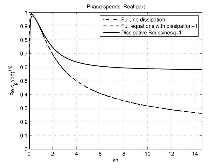
Figure 2: Dissipation model I. Real part of the phase velocity.

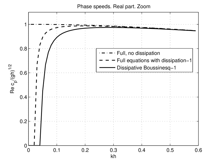
Figure 3: Dissipation model I. Same as Figure 2 with a zoom on long waves.

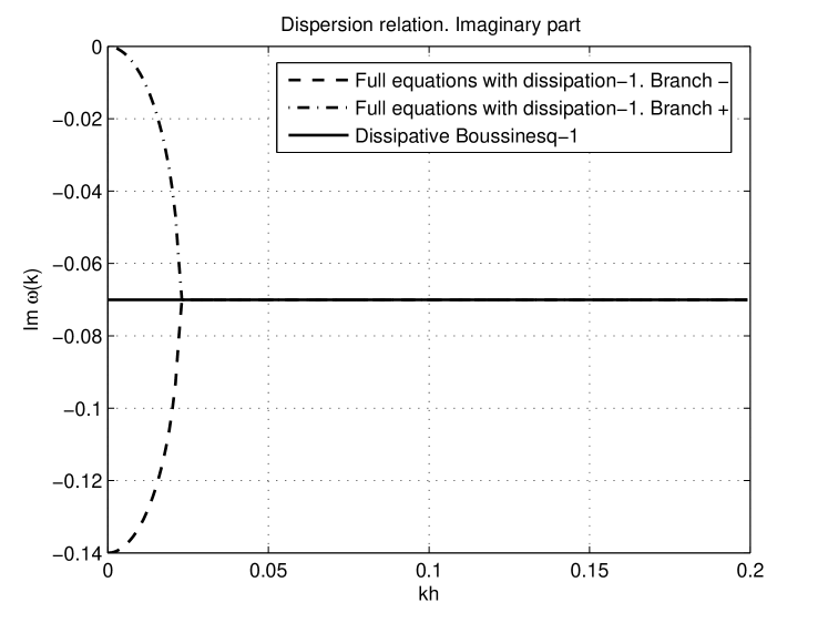
Figure 4: Dissipation model I. Imaginary part of the frequency.

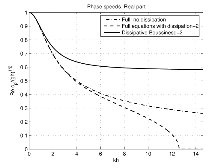
Figure 5: Dissipation model II. Real part of the phase velocity.

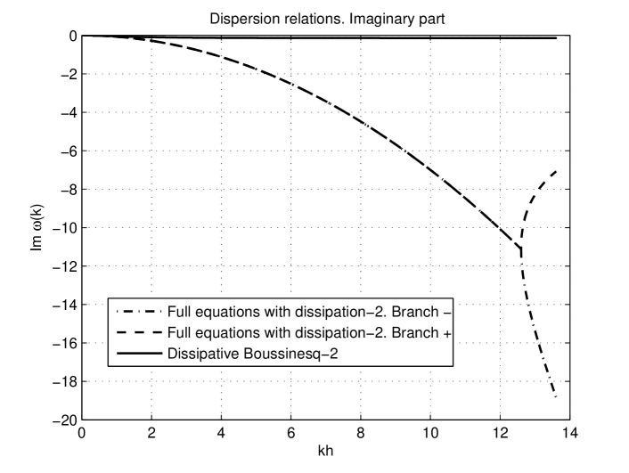
Figure 6: Dissipation model II. Imaginary part of the frequency.

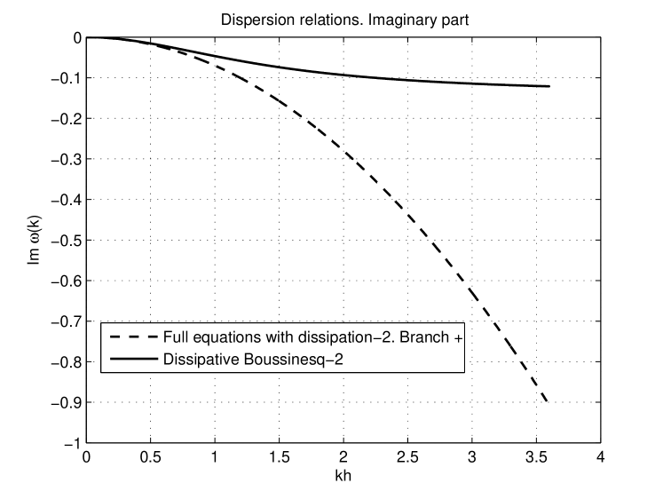
Figure 7: Dissipation model II. Same as Figure 6 with a zoom on long waves.

3.3 Discussion

Let us now provide a discussion on the dispersion relations. The real and imaginary parts of the phase velocities (33)–(36) for the full and long wave linearized equations are shown graphically on Figures 2–7. In this example the parameters are given by $\delta_{1}=0.14,\delta_{2}=0.14$. Together with the dissipative models we also plotted for comparison the well-known phase velocity corresponding to the full conservative (linearized) water-wave problem:

$$c_{p}(k)=\sqrt{gh\frac{\tanh(kh)}{kh}}.$$

First of all, one can see that dissipation is very selective, as is often the case in physics. Clearly, the first dissipation model prefers very long waves, while the second model dissipates essentially short waves. Moreover one can see from the expressions (33), (35) that the phase velocity has a $1/k$ singular behaviour in the vicinity of $kh=0$ (in the long wave limit). Furthermore, it can be clearly seen in Figure 3 that very long linear waves are not advected in the first dissipation model, since the real part of their phase velocity is identically equal to zero.

That is why we suggest to make use of the second model in applications involving very long waves such as tsunamis.

On the other hand we would like to point out that the second model admits a critical wavenumber $k_{c}$ such that the phase velocity (34) becomes purely imaginary with negative imaginary part. From a physical point of view it means that the waves shorter than $k_{c}$ are not advected, but only dissipated. When one switches to the Boussinesq approximation, this property disappears for physically realistic values of the parameters $g$, $h$ and $\delta_{2}$ (see Table 1).

Let us clarify this situation. The qualitative behaviour of the phase velocity $c_{pb}^{(2)}$ (see equation (36)) depends on the roots of the following polynomial equation:

$$(kh)^{4}+\left(8-\frac{3\delta_{2}^{2}}{gh^{3}}\right)(kh)^{2}+12=0.$$

This equation does not have real roots since $\frac{3\delta_{2}^{2}}{gh^{3}}\ll 1$.

4 Alternative version of the Boussinesq equations

In this section we give an alternative derivation of Boussinesq equations. We use another classical method for deriving Boussinesq-type equations (Whitham, 1999; Benjamin, 1974; Peregrine, 1972), which provides slightly different governing equations. Namely, the hyperbolic structure is the same, but the dispersive terms differ. In numerical simulations we suggest to use this system of equations.

The derivation follows closely the paper by Madsen and Schaffer (1998). The main differences are that we neglect the terms of order $O(\mu^{4})$, take in account a moving bathymetry and, of course, dissipative effects which are modelled this time according to model II (4) because, in our opinion, this model is more appropriate for long wave applications. Anyhow, the derivation process can be performed in a similar fashion for model I (3).

4.1 Derivation of the equations

The starting point is the same: equations (5), (6), (7) and (8). This time the procedure begins with representing the velocity potential $\phi(x,y,z,t)$ as a formal expansion in powers of $z$ rather than of $\mu^{2}$:

$$\phi(x,y,z,t)=\sum_{n=0}^{\infty}z^{n}\phi_{n}(x,y,t).$$ (37)

We would like to emphasize that this expansion is only formal and no convergence result is needed. In other words, it is just convenient to use this notation in asymptotic expansions but in practice, seldom more than four terms are used. It is not necessary to justify the convergence of the sum with three or four terms.

When we substitute the expansion (37) into Laplace equation (5), we have an infinite polynomial in $z$. Requiring that $\phi$ formally satisfies Laplace equation implies that the coefficients of each power of $z$ vanish (since the right-hand side is identically zero). This leads to the classical recurrence relation

$$\phi_{n+2}(x,y,t)=-\frac{\mu^{2}}{(n+1)(n+2)}\nabla^{2}\phi_{n}(x,y,t),\qquad n=0,1,2,\ldots$$

Using this relation one can eliminate all but two unknown functions in (37):

$$\phi(x,y,z,t)=\sum_{n=0}^{\infty}(-1)^{n}\mu^{2n}\left(\frac{z^{2n}}{(2n)!}\nabla^{2n}\phi_{0}+\frac{z^{2n+1}}{(2n+1)!}\nabla^{2n}\phi_{1}\right).$$

The following notation is introduced:

$$\mathbf{u}_{0}:=\mathbf{u}(x,y,0,t),\qquad w_{0}:=\frac{1}{\mu^{2}}w(x,y,0,t).$$

It is straightforward to find the relations between $\mathbf{u}_{0}$, $w_{0}$ and $\phi_{0}$, $\phi_{1}$ if one remembers that $(\mathbf{u},w)=(\nabla,\frac{\partial}{\partial z})\phi$:

$$\mathbf{u}_{0}=\nabla\phi_{0},\qquad w_{0}=\frac{1}{\mu^{2}}\phi_{1}.$$

Using the definition of the velocity potential $\phi$ one can express the velocity field in terms of $\mathbf{u}_{0}$, $w_{0}$:

$$\mathbf{u}=\sum_{n=0}^{\infty}(-1)^{n}\left(\frac{z^{2n}}{(2n)!}\mu^{2n}\nabla\bigl{(}\nabla^{2n-2}(\nabla\cdot\mathbf{u}_{0})\bigr{)}+\frac{z^{2n+1}}{(2n+1)!}\mu^{2n+2}\nabla\bigl{(}\nabla^{2n}w_{0}\bigr{)}\right),$$

$$w=\sum_{n=0}^{\infty}(-1)^{n}\left(-\frac{z^{2n+1}}{(2n+1)!}\mu^{2n+2}\nabla^{2n}(\nabla\cdot\mathbf{u}_{0})+\frac{z^{2n}}{(2n)!}\mu^{2n+2}\nabla^{2n}w_{0}\right).$$

These formulas are exact but not practical. In the present work we neglect the terms of order $O(\mu^{4})$ and higher. In this asymptotic framework the above formulas become much simpler:

$$\phi=\phi_{0}+z\phi_{1}-\frac{\mu^{2}z^{2}}{2}\left(\nabla^{2}\phi_{0}+\frac{z}{3}\nabla^{2}\phi_{1}\right)+O(\mu^{4}),$$ (38)

$$\mathbf{u}=\mathbf{u}_{0}+z\mu^{2}\nabla w_{0}-\frac{\mu^{2}z^{2}}{2}\nabla(\nabla\cdot\mathbf{u}_{0})+O(\mu^{4}),$$ (39)

$$w=\mu^{2}w_{0}-z\mu^{2}\nabla\cdot\mathbf{u}_{0}+O(\mu^{4}).$$ (40)

In order to establish the relation between $w_{0}$ and $\mathbf{u}_{0}$ one uses the bottom kinematic boundary condition (8), which has the following form after substituting the asymptotic expansions (38), (39), (40) in it:

$$h_{t}+\varepsilon\nabla h\cdot\Bigl{(}\mathbf{u}_{0}-h\mu^{2}\nabla w_{0}-\frac{\mu^{2}h^{2}}{2}\nabla(\nabla\cdot\mathbf{u}_{0})\Bigr{)}\\ +\varepsilon\Bigl{(}w_{0}-\frac{h^{3}}{6}\mu^{2}\nabla^{2}(\nabla\cdot\mathbf{u}_{0})-\frac{\mu^{2}h^{2}}{2}\nabla^{2}w_{0}\Bigr{)}+O(\mu^{4})=0.$$ (41)

In order to obtain the expression of $w_{0}$ in terms of $\mathbf{u}_{0}$ one introduces one more expansion:

$$w_{0}(x,y,t)=w_{0}^{(0)}(x,y,t)+\mu^{2}w_{0}^{(1)}(x,y,t)+\ldots.$$ (42)

We insert this expansion into the asymptotic bottom boundary condition (41). This leads to the following explicit expressions for $w_{0}^{(0)}$ and $w_{0}^{(1)}$:

$$w_{0}^{(0)}=-\frac{1}{\varepsilon}h_{t}-\nabla\cdot(h\mathbf{u}_{0}),$$

$$w_{0}^{(1)}=\frac{h^{2}}{2}\Bigl{(}\nabla h\cdot\nabla(\nabla\cdot\mathbf{u}_{0})+\frac{h}{3}\nabla^{2}(\nabla\cdot\mathbf{u}_{0})\Bigr{)}\\ -h\left(\nabla h\cdot\frac{1}{\varepsilon}\nabla h_{t}+\nabla h\cdot\nabla\bigl{(}\nabla\cdot(h\mathbf{u}_{0})\bigr{)}+\frac{h}{2}\bigl{(}\frac{1}{\varepsilon}\nabla^{2}h_{t}+\nabla^{2}(\nabla\cdot(h\mathbf{u}_{0}))\bigr{)}\right).$$

Substituting these expansions into (42) and performing some simplifications yields the required relation between $\mathbf{u}_{0}$ and $w_{0}$:

$$w_{0}=-\frac{1}{\varepsilon}h_{t}-\nabla\cdot(h\mathbf{u}_{0})\\ -\mu^{2}\nabla\cdot\Bigl{(}\frac{h^{2}}{2\varepsilon}\nabla h_{t}+\frac{h^{2}}{2}\nabla\bigl{(}\nabla\cdot(h\mathbf{u}_{0})\bigr{)}-\frac{h^{3}}{6}\nabla(\nabla\cdot\mathbf{u}_{0})\Bigr{)}+O(\mu^{4}).$$ (43)

Now one can eliminate the vertical velocity $w_{0}$ since one has its expression (43) in terms of $\mathbf{u}_{0}$. Equations (39)-(40) become

$$\mathbf{u}=\mathbf{u}_{0}-z\frac{\mu^{2}}{\varepsilon}\nabla h_{t}-\mu^{2}\Bigl{(}z\nabla\bigl{(}\nabla\cdot(h\mathbf{u}_{0})\bigr{)}+\frac{z^{2}}{2}\nabla(\nabla\cdot\mathbf{u}_{0})\Bigr{)}+O(\mu^{4}),$$ (44)

$$w=-\frac{\mu^{2}}{\varepsilon}h_{t}-\mu^{2}\Bigl{(}\nabla\cdot(h\mathbf{u}_{0})+z\nabla\cdot\mathbf{u}_{0}\Bigr{)}+O(\mu^{4}).$$ (45)

In this work we apply a trick due to Nwogu (1993). Namely, we introduce a new velocity variable $\mathbf{u_{\alpha}}$ defined at an arbitrary water level $z_{\alpha}=-\alpha h$. Technically this change of variables is done as follows. First we evaluate (44) at $z=z_{\alpha}$, which gives the connection between $\mathbf{u}_{0}$ and $\mathbf{u_{\alpha}}$:

$$\mathbf{u_{\alpha}}=\mathbf{u}_{0}-z_{\alpha}\frac{\mu^{2}}{\varepsilon}\nabla h_{t}-\mu^{2}\Bigl{(}z_{\alpha}\nabla\bigl{(}\nabla\cdot(h\mathbf{u}_{0})\bigr{)}+\frac{z_{\alpha}^{2}}{2}\nabla(\nabla\cdot\mathbf{u}_{0})\Bigr{)}+O(\mu^{4}).$$

Using the standard technics of inversion one can rewrite the last expression as an asymptotic formula for $\mathbf{u}_{0}$ in terms of $\mathbf{u_{\alpha}}$:

$$\mathbf{u}_{0}=\mathbf{u_{\alpha}}+z_{\alpha}\frac{\mu^{2}}{\varepsilon}h_{t}+\mu^{2}\Bigl{(}z_{\alpha}\nabla\bigl{(}\nabla\cdot(h\mathbf{u_{\alpha}})\bigr{)}+\frac{z_{\alpha}^{2}}{2}\nabla(\nabla\cdot\mathbf{u_{\alpha}})\Bigr{)}+O(\mu^{4}).$$ (46)

Remark: Behind this change of variables there is one subtlety which is generally hushed up in the literature. In fact, the wave motion is assumed to be irrotational since we use the potential flow formulation (5), (6), (7), (8) of the water-wave problem. By construction $\mathop{\mathrm{rot}}(\mathbf{u},w)=\mathbf{0}$ when $\mathbf{u}$ and $w$ are computed according to (44), (45) or, in other words, in terms of the variable $\mathbf{u}_{0}$. When one turns to the velocity variable $\mathbf{u_{\alpha}}$ defined at an arbitrary level, one can improve the linear dispersion relation and this is important for wave modelling. But on the other hand, one loses the property that the flow is irrotational. That is to say, a direct computation shows that $\mathop{\mathrm{rot}}(\mathbf{u},w)\neq\mathbf{0}$ when $\mathbf{u}$ and $w$ are expressed in terms of the variable $\mathbf{u_{\alpha}}$. The purpose of this remark is simply to inform the reader about the price to be paid while improving the dispersion relation properties. It seems that this point is not clearly mentioned in the literature on this topic.

Let us now derive the Boussinesq equations. There are two different methods to obtain the free-surface elevation equation. The first method consists in integrating the continuity equation (5) over the depth and then use the kinematic free-surface and bottom boundary conditions. The second way is more straightforward. It consists in using directly the kinematic free-surface boundary condition (6):

$$\eta_{t}+\varepsilon\nabla\phi\cdot\nabla\eta-\frac{1}{\mu^{2}}\phi_{z}=0.$$

Then one can substitute (38) into (6) and perform several simplifications. Neglecting all terms of order $O(\varepsilon^{2}+\varepsilon\mu^{2}+\mu^{4})$ yields the following equation :

$$\eta_{t}+\nabla\cdot\bigl{(}(h+\varepsilon\eta)\mathbf{u}_{0}\bigr{)}+\frac{\mu^{2}}{2}\nabla\cdot\Bigl{(}h^{2}\nabla\bigl{(}\nabla\cdot(h\mathbf{u}_{0})\bigr{)}-\frac{h^{3}}{3}\nabla(\nabla\cdot\mathbf{u}_{0})\Bigr{)}=\\ =\zeta_{t}+\frac{\mu^{2}}{2}\nabla\cdot(h^{2}\nabla\zeta_{t}).$$

Recall that $\zeta(x,y,t)$ is defined according to (20). When the bathymetry is static, $\zeta\equiv 0$. We prefer to introduce this function in order to eliminate the division by $\varepsilon$ in the source terms since this division can give the impression that stiff source terms are present in our problem, which is not the case.

In order to be able to optimize the dispersion relation properties, we switch to the variable $\mathbf{u_{\alpha}}$. Technically it is done by using the relation (46) between $\mathbf{u}_{0}$ and $\mathbf{u_{\alpha}}$. The result is given below:

$$\eta_{t}+\nabla\cdot\bigl{(}(h+\varepsilon\eta)\mathbf{u_{\alpha}}\bigr{)}+\mu^{2}\nabla\cdot\Bigl{(}h\bigl{(}z_{\alpha}+\frac{h}{2}\bigr{)}\nabla\bigl{(}\nabla\cdot(h\mathbf{u_{\alpha}})\bigr{)}+\frac{h}{2}\bigl{(}z_{\alpha}^{2}-\frac{h^{2}}{3}\bigr{)}\nabla(\nabla\cdot\mathbf{u_{\alpha}})\Bigr{)}=\\ =\zeta_{t}+\mu^{2}\nabla\cdot\Bigl{(}h\bigl{(}z_{\alpha}+\frac{h}{2}\bigr{)}\nabla\zeta_{t}\Bigr{)}.$$ (47)

As above, the equation for the horizontal velocity field is derived from the dynamic free-surface boundary condition (7). It is done exactly as in section 2 and we do not insist on this point:

$$\mathbf{u}_{0t}+\frac{\varepsilon}{2}\nabla\left|\mathbf{u}_{0}\right|^{2}+\nabla\eta-\varepsilon\delta\nabla^{2}\mathbf{u}_{0}=\mathbf{0}.$$

Switching to the variable $\mathbf{u_{\alpha}}$ yields the following governing equation:

$$\mathbf{u_{\alpha}}_{t}+\frac{\varepsilon}{2}\nabla|\mathbf{u_{\alpha}}|^{2}+\nabla\eta+\mu^{2}\Bigl{(}z_{\alpha}\nabla\bigl{(}\nabla\cdot(h\mathbf{u_{\alpha}})\bigr{)}+\frac{z_{\alpha}^{2}}{2}\nabla(\nabla\cdot\mathbf{u_{\alpha}})\Bigr{)}_{t}=\\ =\varepsilon\delta\Delta\mathbf{u_{\alpha}}+\mu^{2}(z_{\alpha}\nabla\zeta_{t})_{t}.$$ (48)

In several numerical methods it can be advantageous to rewrite the system (47), (48) in vector form:

$$\mathbf{U}_{t}+\mu^{2}\mathbf{L}(\mathbf{U})_{t}+\nabla\cdot\mathbf{F}(\mathbf{U})+\mu^{2}\nabla\cdot\mathbf{P}(\mathbf{U})=\mathbf{S}(x,y,t)+\varepsilon\delta\nabla\cdot(\mathbf{D}\nabla\mathbf{U})),$$

where

$$\mathbf{U}:=\begin{pmatrix}\eta\\ u_{\alpha}\\ v_{\alpha}\end{pmatrix},\quad\nabla\cdot\mathbf{F}:=\frac{\partial F}{\partial x}+\frac{\partial G}{\partial y},$$

$$F:=\begin{pmatrix}(h+\varepsilon\eta)u_{\alpha}\\ \frac{\varepsilon}{2}|\mathbf{u_{\alpha}}|^{2}+\eta\\ 0\end{pmatrix},\quad G:=\begin{pmatrix}(h+\varepsilon\eta)v_{\alpha}\\ 0\\ \frac{\varepsilon}{2}|\mathbf{u_{\alpha}}|^{2}+\eta\\ \end{pmatrix},$$

$$\mathbf{L}:=\begin{pmatrix}0\\ z_{\alpha}\nabla\bigl{(}\nabla\cdot(h\mathbf{u_{\alpha}})\bigr{)}+\frac{z_{\alpha}^{2}}{2}\nabla(\nabla\cdot\mathbf{u_{\alpha}})\end{pmatrix},$$

$$\mathbf{P}:=\begin{pmatrix}h\bigl{(}z_{\alpha}+\frac{h}{2}\bigr{)}\nabla\bigl{(}\nabla\cdot(h\mathbf{u_{\alpha}})\bigr{)}+\frac{h}{2}\bigl{(}z_{\alpha}^{2}-\frac{h^{2}}{3}\bigr{)}\nabla(\nabla\cdot\mathbf{u_{\alpha}})\\ \mathbf{0}\end{pmatrix},$$

$$\mathbf{S}:=\begin{pmatrix}\zeta_{t}+\mu^{2}\nabla\cdot\Bigl{(}h\bigl{(}z_{\alpha}+\frac{h}{2}\bigr{)}\nabla\zeta_{t}\Bigr{)}\\ \mu^{2}(z_{\alpha}\nabla\zeta_{t})_{t}\end{pmatrix},$$

$$\mathbf{D}:=\begin{pmatrix}0&0&0\\ 0&1&0\\ 0&0&1\\ \end{pmatrix}.$$

4.2 Improvement of the linear dispersion relations

As said above, the idea of using one free parameter $\alpha\in[0,1]$ to optimize the linear dispersion relation properties appears to have been proposed first by Nwogu (1993).

The idea of manipulating the dispersion relation was well-known before 1993. See for example Murray (1989); Madsen et al. (1991). But these authors started with a desired dispersion relation and artificially added extra terms to the momentum equation in order to produce the desired characteristics. We prefer to follow the ideas of Nwogu (1993).

Remark: When one plays with the dispersion relation it is important to remember that the resulting problem must be well-posed, at least linearly. We refer to Bona et al. (2002) as a general reference on this topic. Usually Boussinesq-type models with good dispersion characteristics are linearly well-posed as well.

In order to look for an optimal value of $\alpha$ we will drop dissipative terms. Indeed we want to concentrate our attention on the propagation properties which are more important.

The choice for the parameter $\alpha$ depends on the optimization criterion. In the present work we choose $\alpha$ by comparing the coefficients in the Taylor expansions of the phase velocity in the vicinity of $kh=0$, which corresponds to the long-wave limit. Another possibility is to match the dispersion relation of the full linearized equations (32) in the least square sense. One can also use Padé approximants (Witting, 1984) since rational functions have better approximation properties than polynomials.

We briefly describe the procedure. First of all one has to obtain the phase velocity of the linearized, non-viscous, Boussinesq equations (47)-(48). The result is

$$\frac{c_{b}^{2}(k)}{gh}=\frac{1-\bigl{(}\frac{\alpha^{2}}{2}-\alpha+\frac{1}{3}\bigr{)}(kh)^{2}}{1-\alpha\bigl{(}\frac{\alpha}{2}-1\bigr{)}(kh)^{2}}=1-\frac{1}{3}(kh)^{2}+\frac{\alpha(2-\alpha)}{6}(kh)^{4}+O\left((kh)^{6}\right).$$ (49)

On the other hand one can write down the phase velocity of the full linearized equations (32):

$$\frac{c^{2}(k)}{gh}=\frac{\tanh(kh)}{kh}=1-\frac{1}{3}(kh)^{2}+\frac{2}{15}(kh)^{4}+O\left((kh)^{6}\right).$$

If one insists on the dispersion relation (49) to be exact up to order $O\left((kh)^{4}\right)$ one immediately obtains an equation for $\alpha_{opt}$:

$$\frac{\alpha_{opt}(2-\alpha_{opt})}{6}=\frac{2}{15}\Rightarrow\alpha_{opt}=1-\frac{\sqrt{5}}{5}\approx 0.55.$$

We suggest using this value of $\alpha$ in numerical computations.

4.3 Bottom friction

In this subsection, one switches back to dimensional variables. It is a common practice in hydraulics engineering to take into account the effect of bottom friction or bottom rugosity. In the Boussinesq and nonlinear shallow water equations there is also a possibility to include some kind of empirical terms to model these physical effects. From the mathematical and especially numerical viewpoints these terms do not add any complexity, since they have the form of source terms that do not involve differential operators. So it is highly recommended to introduce these source terms in numerical models.

There is no unique bottom friction law. Most frequently, Chézy and Darcy-Weisbach laws are used. Both laws have similar structures. We give here these models in dimensional form. The following terms have to be added to the source terms of Boussinesq equations when one wants to include bottom friction modelling.

• Chézy law:

  $$\mathbf{S}_{f}=-C_{f}g\frac{\mathbf{u}\left|\mathbf{u}\right|}{h+\eta},$$

  where $C_{f}$ is the Chézy coefficient.

• Darcy-Weisbach law:

  $$\mathbf{S}_{f}=-\frac{\lambda\mathbf{u}\left|\mathbf{u}\right|}{8(h+\eta)},$$

  where $\lambda$ is the so-called resistance value. This parameter is determined according to the simplified form of the Colebrook-White relation:

  $$\frac{1}{\sqrt{\lambda}}=-2.03\log\left(\frac{k_{s}}{14.84(h+\eta)}\right).$$

  Here $k_{s}$ denotes the friction parameter, which depends on the composition of the bottom. Typically $k_{s}$ can vary from $1$mm for concrete to $300$mm for bottom with dense vegetation.

• Manning-Strickler law:

  $$\mathbf{S}_{f}=-k^{2}g\frac{\mathbf{u}\left|\mathbf{u}\right|}{(h+\eta)^{\frac{4}{3}}},$$

  where $k$ is the Manning roughness coefficient.

5 Spectral Fourier method

In this study we adopted a well-known and widely used spectral Fourier method. The main idea consists in discretizing the spatial derivatives using Fourier transforms. The effectiveness of this method is explained by two main reasons. First, the differentiation operation in Fourier transform space is extremely simple due to the following property of Fourier transforms: $\overline{f^{\prime}}=ik\overline{f}$. Secondly, there are very powerful tools for the fast and accurate computation of discrete Fourier transforms (DFT). So, spatial derivatives are computed with the following algorithm:

1:  $\overline{f}\leftarrow{\rm fft}\,(f)$

2:  $\overline{v}\leftarrow ik\overline{f}$

3:  $f^{\prime}\leftarrow{\rm ifft}\,(\overline{v})$

where $k$ is the wavenumber.

This approach, which is extremely efficient, has the drawbacks of almost all spectral methods. The first drawback consists in imposing periodic boundary conditions since we use DFT. The second drawback is that we can only handle simple geometries, namely, Cartesian products of $1$D intervals. For the purpose of academic research, this type of method is appropriate.

Let us now consider the discretization of the dissipative Boussinesq equations. We show in detail how the discretization is performed on equations (22), (24). The other systems are discretized in the same way. We chose equations (22), (24) in order to avoid cumbersome expressions and make the description as clear as possible.

Let us apply the Fourier transform to both sides of equations (22), (24):

$$\overline{\eta}_{t}=-i\mathbf{k}\cdot\overline{(h+\varepsilon\eta)\mathbf{u}}-\frac{1}{\varepsilon}\overline{h}_{t}-\frac{\mu^{2}}{2\varepsilon}\overline{h^{2}\nabla^{2}h_{t}}-\frac{\mu^{2}}{\varepsilon}\overline{h\nabla h\cdot\nabla h_{t}}+\frac{\mu^{2}}{6}\overline{h^{3}\nabla^{2}\nabla\cdot\mathbf{u}}\\ +\frac{\mu^{2}}{2}\overline{h^{2}\nabla^{2}h\nabla\cdot\mathbf{u}}+\mu^{2}\overline{h\left|\nabla h\right|^{2}\nabla\cdot\mathbf{u}}+\mu^{2}\overline{h^{2}\nabla h\cdot\nabla(\nabla\cdot\mathbf{u})},$$ (50)

$$\overline{\mathbf{u}}_{t}+\frac{1}{2}{\varepsilon}i\mathbf{k}\overline{\left|\mathbf{u}\right|^{2}}+i\mathbf{k}\overline{\eta}+\varepsilon\nu_{2}\left|\mathbf{k}\right|^{2}\overline{\mathbf{u}}-\frac{1}{2}\mu^{2}i\mathbf{k}\overline{h^{2}\nabla\cdot\mathbf{u}_{t}}=0,$$ (51)

where $\mathbf{k}=(k_{x},k_{y})$ denotes the Fourier transform parameters.

Equations (50) and (51) constitute a system of ordinary differential equations to be integrated numerically. In the present study we use the classical explicit fourth-order Runge-Kutta method.

Remark on stability: A lot of researchers who integrated numerically the KdV equation noticed that the stability criterion has the form

$$\Delta t=\frac{\lambda}{N^{2}},$$

where $\lambda$ is the Courant-Friedrichs-Lewy (CFL) number and $N$ the number of points of discretization. In order to increase the time integration step $\Delta t$ they solved exactly the linear part of the partial differential equation since the linear term is the one involving high frequencies and constraining the stability. This method, which is usually called the integrating factor method, allows an increase of the CFL number up to a factor ten, but it cannot fix the dependence on $1/N^{2}$.

We do not have this difficulty because we use regularized dispersive terms. The regularization effect can be seen from equation (51). The same idea was exploited by Bona et al. (1981), who used the modified KdV equation (9).

Let us briefly explain how we treat the non-linear terms. Since the time integration scheme is explicit, one can easily handle nonlinearities. For example the term $\overline{(h+\varepsilon\eta)\mathbf{u}}$ is computed as follows:

$$\overline{(h+\varepsilon\eta)\mathbf{u}}={\rm fft}\,\left((h+\varepsilon\mathop{\mathrm{Re}}{\rm ifft}\,(\overline{\eta}))\cdot\mathop{\mathrm{Re}}{\rm ifft}\,(\overline{\mathbf{u}})\right).$$

The other nonlinear terms are computed in the same way.

5.1 Validation of the numerical method

One way to validate a numerical scheme is to compare the numerical results with analytical solutions. Unfortunately, the authors did not succeed in deriving analytical solutions to the $(1+1)$D dissipative Boussinesq equations over a flat bottom. But for validation purposes, one can neglect the viscous term. With this simplification several solitary wave solutions can be obtained. We follow closely the work of Chen (1998). In $(1+1)$D in the presence of a flat bottom, the Boussinesq system without dissipation becomes

$$\eta_{t}+u_{x}+\varepsilon(u\eta)_{x}-\frac{\mu^{2}}{6}u_{xxx}=0,$$ (52)

$$u_{t}+\eta_{x}+\varepsilon uu_{x}-\frac{\mu^{2}}{2}u_{xxt}=0.$$ (53)

We look for solitary-wave solutions travelling to the left in the form

$$\eta(x,t)=\eta(\xi)=\eta(x_{0}+x+ct),\qquad u(x,t)=B\eta(\xi),$$

where we introduced the new variable $\xi=x_{0}+x+ct$ and $B$, $c$, $x_{0}$ are constants. From the physical point of view this change of variables is nothing else than Galilean transformation. In other words we choose a new frame of reference which moves with the same celerity as the solitary wave. Since $c$ is constant (there is no acceleration), the observer moving with the wave will see a steady picture.

In the following primes denote derivation with respect to $\xi$. Substituting this special form into the governing equations (52)-(53) gives

$$c\eta^{\prime}+u^{\prime}+\varepsilon(u\eta)^{\prime}-\frac{\mu^{2}}{6}u^{\prime\prime\prime}=0,$$

$$cu^{\prime}+\eta^{\prime}+\varepsilon uu^{\prime}-c\frac{\mu^{2}}{2}u^{\prime\prime\prime}=0.$$

One can decrease the order of derivatives by integrating once:

$$c\eta+u+\varepsilon u\eta-\frac{\mu^{2}}{6}u^{\prime\prime}=0,$$

$$cu+\eta+\frac{\varepsilon}{2}u^{2}-c\frac{\mu^{2}}{2}u^{\prime\prime}=0.$$

The solution is integrable on $\mathbb{R}$ and there are no integration constants, since a priori the solution behaviour at infinity is known: the solitary wave is exponentially small at large distances from the crest. Mathematically it can be expressed as

$$\lim_{\xi\to\pm\infty}\eta(x,t)=\lim_{\xi\to\pm\infty}u(x,t)=0.$$

Now we use the relation $u(\xi)=B\eta(\xi)$ to eliminate the variable $u$ from the system:

$$(c+B)\eta-B\frac{\mu^{2}}{6}\eta^{\prime\prime}=-\varepsilon B\eta^{2},$$ (54)

$$(1+cB)\eta-cB\frac{\mu^{2}}{2}\eta^{\prime\prime}=-\frac{\varepsilon}{2}B^{2}\eta^{2}.$$ (55)

In order to have non-trivial solutions both equations must be compatible. Compatibility conditions are obtained by comparing the coefficients of corresponding terms in equations (54)-(55):

$$\frac{1}{2}B^{2}-\frac{1}{2}Bc = 1,$$

$$\frac{1}{6}B^{2}-Bc = 0.$$

These relations can be thought as a system of linear equations with respect to $B^{2}$ and $Bc$. The unique solution of those equations is

$$B^{2}=\frac{12}{5},\quad c=\frac{B}{6}.$$

Choosing $B>0$ so that $c>0$ leads to

$$B=\frac{6}{\sqrt{15}},\quad c=\frac{1}{\sqrt{15}}.$$

These constants determine the amplitude and the propagation speed of the solitary wave. In order to find the shape of the wave, one differentiates once equation (55):

$$7\eta^{\prime}-\mu^{2}\eta^{\prime\prime\prime}=-12\varepsilon\eta\eta^{\prime}.$$ (56)

The solution to this equation is well-known (see for example Newell (1977); Chen (1998)):

Lemma 1.

Let $\alpha$, $\beta$ be real constants; the equation

$$\alpha\eta^{\prime}(\xi)-\beta\eta^{\prime\prime\prime}(\xi)=\eta(\xi)\eta^{\prime}(\xi)$$

has a solitary-wave solution if $\alpha\beta>0$. Moreover, the solitary-wave solution is

$$\eta(\xi)=3\alpha\,{\rm sech}\,^{2}\left(\frac{1}{2}\sqrt{\frac{\alpha}{\beta}}(\xi+\xi_{0})\right)$$

where $\xi_{0}$ is an arbitrary constant.

Applying this lemma to equation (56) yields the following solution:

$$\eta(x,t)=-\frac{7}{4\varepsilon}\,{\rm sech}\,^{2}\left(\frac{\sqrt{7}}{2\mu}(x+ct+x_{0})\right),$$ (57)

$$u(x,t)=-\frac{7\sqrt{15}}{10\varepsilon}\,{\rm sech}\,^{2}\left(\frac{\sqrt{7}}{2\mu}(x+ct+x_{0})\right).$$

Note that this exact solitary wave solution is not physical. Indeed the velocity is negative whereas one expects it to be positive for a depression wave propagating to the left. In any case, the goal here is to validate the numerical computations by comparing with an exact solution. The methodology is simple. We choose a solitary wave as initial condition and let it propagate during a certain time $T$ with the spectral method. At the end of the computations one computes the $L_{\infty}$ norm of the difference between the analytical solution (57) and the numerical one $\tilde{\eta}(x,T)$:

$$\epsilon_{N}:=\max_{1\leq i\leq N}\left|\eta(x_{i},T)-\tilde{\eta}(x_{i},T)\right|,$$

where $\left\{x_{i}\right\}_{1\leq i\leq N}$ are the discretization points.

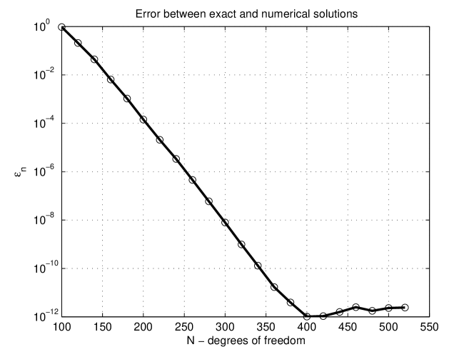
Figure 8: Error on the numerical computation of a solitary wave solution. Here $T=1$.

Figure 8 shows the graph of $\epsilon_{N}$ as a function of $N$. This result shows an excellent performance of this spectral method with an exponential convergence rate. In general, the error $\epsilon_{N}$ is bounded below by the maximum between the error due to the time integration algorithm and floating point arithmetic precision.

The exponential convergence rate to the exact solution is one of the features of spectral methods. It explains the success of these methods in several domains such as direct numerical simulation (DNS) of turbulence. One of the main drawbacks of spectral methods consists in the difficulties in handling complex geometries and various types of boundary conditions.

6 Numerical results

In this section we perform comparisons between the two dissipation models (23) and (24). Even though the computations we show deal with a 1D wave propagating in the negative $x-$direction, they have been performed with the 2D version of the code. The bathymetry $z=-h(x,y)$ is chosen to be a regularized step function which is translated in the $y-$direction. A typical function $h(x,y)$ is given by

$$h(x)=\left\{\begin{array}[]{lc}h_{l},&x\leq x_{0},\\ h_{l}+\frac{1}{2}(h_{r}-h_{l})\left(1+\sin\left(\frac{\pi}{\Delta x}(x-x_{0}-\frac{1}{2}\Delta x)\right)\right),&x_{0}<x<x_{0}+\Delta x,\\ h_{r},&x\geq x_{0}+\Delta x.\end{array}\right.$$ (58)

This test case is interesting from a practical point of view since it clearly illustrates the phenomena of long wave reflection by bottom topography. The parameters used in this computation are given in Table 2. All values are given in nondimensional form.

parameter	$h_{l}$	$h_{r}$	$x_{0}$	$\Delta x$	$\varepsilon$	$\mu$	$\nu_{1}$, $\nu_{2}$
value	0.5	1.0	$-0.5$	0.3	0.005	0.06	0.14

Table 2: Typical values of the parameters used in the numerical computations

6.1 Construction of the initial condition

We propagate on the free surface a so-called approximate soliton. Its classical construction is as follows. We begin with the non-dissipative Boussinesq equations on a flat bottom:

$$\eta_{t}+\bigl{(}(1+\varepsilon\eta)u\bigr{)}_{x}-\frac{\mu^{2}}{6}u_{xxx}=0,$$

$$u_{t}+\eta_{x}+\frac{\varepsilon}{2}(u^{2})_{x}-\frac{\mu^{2}}{2}u_{xxt}=0,$$ (59)

and look for $u$ in the following form:

$$u=-\eta+\varepsilon P+\mu^{2}Q+O(\varepsilon^{2}+\varepsilon\mu^{2}+\mu^{4}).$$ (60)

It is precisely at this step that one makes an approximation. One substitutes this asymptotic expansion into the governing equations and retains only the terms of order $O(\varepsilon+\mu^{2})$:

$$\eta_{t}-\eta_{x}+\varepsilon P_{x}+\mu^{2}Q_{x}-2\varepsilon\eta\eta_{x}+\frac{\mu^{2}}{6}\eta_{xxx}=O(\varepsilon^{2}+\varepsilon\mu^{2}+\mu^{4}),$$ (61)

$$-\eta_{t}+\eta_{x}+\varepsilon P_{t}+\mu^{2}Q_{t}+\varepsilon\eta\eta_{x}+\frac{\mu^{2}}{2}\eta_{xxt}=O(\varepsilon^{2}+\varepsilon\mu^{2}+\mu^{4}).$$

Add these two equations and set the coefficients of $\varepsilon$ and $\mu^{2}$ equal to 0:

$$\varepsilon: P_{x}+P_{t}-\eta\eta_{x}=0,$$ (62)

$$\mu^{2}: Q_{x}+Q_{t}+\frac{1}{6}\eta_{xxx}+\frac{1}{2}\eta_{xxt}=0.$$ (63)

Since the water depth is $h=1+\varepsilon\eta=1+O(\varepsilon)$, the approximate solitary wave should travel to the left with a celerity $c=1+O(\varepsilon)$ and depend on the variable $x+ct=x+t+O(\varepsilon)$. Consequently one has the following relations:

$$\frac{\partial f}{\partial t}=\frac{\partial f}{\partial x}+O(\varepsilon+\mu^{2}),\qquad f\in\{\eta,P,Q\}.$$

Replacing time derivatives by spatial ones in (62)-(63) yields

$$P_{x}=\frac{1}{2}\eta\eta_{x},\qquad Q_{x}=-\frac{1}{3}\eta_{xxx}.$$

By integration (using the fact that solitary waves tend to zero at infinity), one obtains

$$P=\frac{1}{4}\eta^{2},\qquad Q=-\frac{1}{3}\eta_{xx}$$ (64)

and the relation (60) connecting $\eta$ and $u$ becomes

$$u=-\eta+\frac{\varepsilon}{4}\eta^{2}-\frac{\mu^{2}}{3}\eta_{xx}+\ldots.$$ (65)

Substituting this expression for $u$ into (61) yields a classical KdV equation for $\eta$:

$$\eta_{t}-\left(1+\frac{3}{2}\varepsilon\eta\right)\eta_{x}-\frac{\mu^{2}}{6}\eta_{xxx}=0,$$ (66)

which admits solitary wave solutions of the form $\eta=\eta(x+ct)$:

$$\eta(x,t)=\frac{2(c-1)}{\varepsilon}{\rm sech}\,^{2}\left(\frac{1}{2\mu}\sqrt{6(c-1)}(x+ct)\right),$$

where $c>1$. The velocity $u$ is obtained from (65) by simple substitution. This approximate soliton is used in the numerical computations.

6.2 Comparison between the dissipative models

The snapshot of the function $\eta(x,y,t_{0})$ (divided by 10 for clarity’s sake) during and just after reflection by the step is given on Figure 9. Recall that the free surface is given by $z=\varepsilon\eta$.

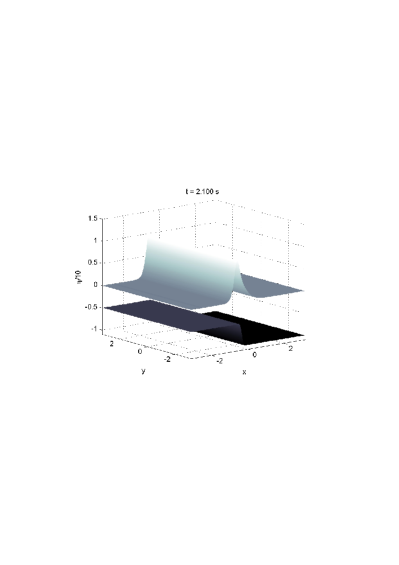
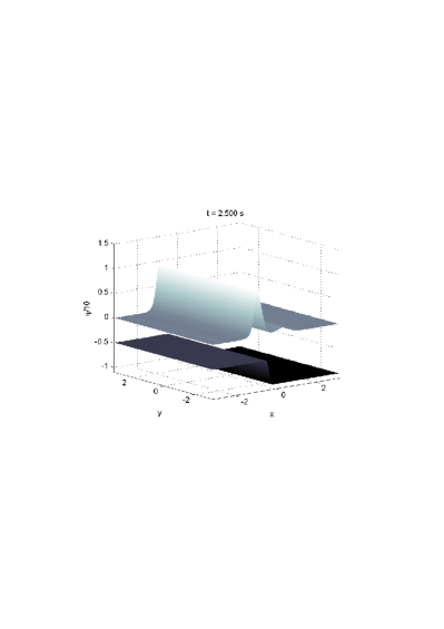
Figure 9: Interaction between a left-running solitary wave and a step at two different times. The plots represent $\eta/10$ while the true free-surface profiles are given by $z=\varepsilon\eta$.

Then we compare the two sets of equations (22), (23) and (22), (24). To do so we look at the section of the free surface at $y=0$ along the propagation direction.

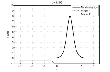
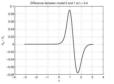
Figure 10: Free-surface snapshot before the interaction with the step: (left) the curves corresponding to the three models are almost superimposed; (right) difference between model II and model I.

Figure 10 shows that even at the beginning of the computations the two models give slightly different results. The amplitude of the pulse obtained with model I is smaller. It can be explained by the presence of the term $\nu_{1}S\mathbf{u}$ which is bigger in magnitude than $\varepsilon\nu_{2}\nabla^{2}\mathbf{u}$. Within graphical accuracy, there is almost no difference between the conservative case and model II.

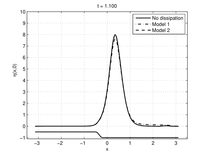
Figure 11: Free surface just before the interaction with the step

In Figure 11 one can see that differences between the two solitons continue to grow. In particular we see an important drawback of the dissipation model I: just after the wave crest the free surface has some kind of residual deformation which is clearly non-physical. Our numerical experiments show that the amplitude of this residue depends almost linearly on the parameter $\nu_{1}$. We could hardly predict this effect directly from the equations without numerical experiments.

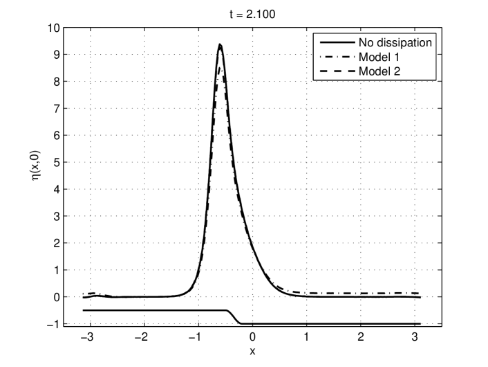
Figure 12: Beginning of the solitary wave deformation under the change in bathymetry

We would like to point out several soliton transformations in Figure 12 due to the interaction with bathymetry. First of all, since the depth decreases, the wave amplitude grows. Quantitatively speaking, the wave amplitude before the interaction is equal exactly to $8$ (without including dissipation) and over the step it becomes roughly $9.4$. On the other hand the soliton becomes less symmetric which is also expected. Because of periodic numerical boundary conditions we also observe the residue of the free-surface deformation coming through the left boundary.

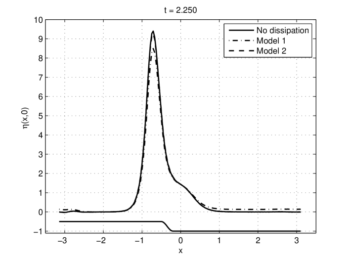
Figure 13: Initiation of the reflected wave separation

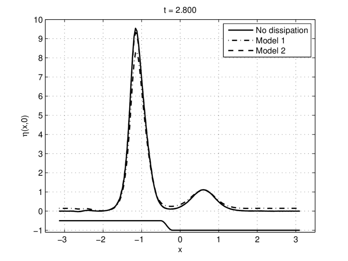
Figure 14: Separation of the reflected wave

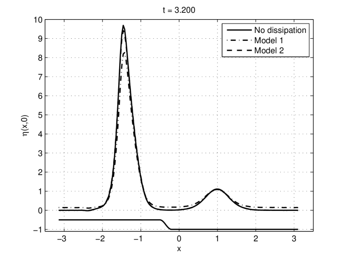
Figure 15: Two separate waves moving in opposite directions

Figures 13, 14 and 15 show the process of wave reflection from the step at the bottom. The reflected wave clearly moves in the opposite direction. The fact that we see almost no difference between Model II and the conservative case should not lead to the interpretation that dissipative effects are not important. One just has to wait long enough to see these effects play a role.

7 Conclusions

Comparisons have been made between two dissipation models. Model II, in which the decay is proportional to the second derivative of the velocity, appears to be better. At this stage we cannot show comparisons with laboratory experiments in order to demonstrate the performance of model II. Nevertheless, there is an indirect evidence. We refer one more time to the theoretical as well as experimental work of Bona et al. (1981). In order to model wave trains, they added to the Korteweg–de Vries equation an ad-hoc dissipative term in the form of the Laplacian (but in 1D). This term coincides with the results of our derivation if we model dissipation in the equations according to the second model. Their work shows excellent agreement between experiments and numerical solutions to dissipative KdV equation. Moreover our dissipative Boussinesq equations are in the same relationship with the classical Boussinesq equations (Peregrine, 1967) as Euler and Navier-Stokes equations. This is a second argument towards the physical pertinency of the results obtained with model II.

References

- Benjamin (1974) T. B. Benjamin. Lectures in Appl. Math., volume 15, chapter Lectures on nonlinear wave motion, pages 3–47. Amer. Math. Soc., Providence, RI, 1974.
- Benoit (2006) M. Benoit. Contribution à l’étude des états de mer et des vagues, depuis l’océan jusqu’aux ouvrages cotiers. 2006. Mémoire d’habilitation à diriger des recherches.
- Bona et al. (1981) J.L. Bona, W.G. Pritchard, and L.R. Scott. An evaluation of a model equation for water waves. Phil. Trans. R. Soc. Lond. A, 302:457–510, 1981.
- Bona et al. (2002) J.L. Bona, M. Chen, and J.-C. Saut. Boussinesq equations and other systems for small-amplitude long waves in nonlinear dispersive media. i: Derivation and linear theory. Journal of Nonlinear Science, 12:283–318, 2002.
- Boussinesq (1872) J. Boussinesq. Théorie des ondes et des remous qui se propagent le long d’un canal rectangulaire horizontal, en communiquant au liquide contenu dans ce canal des vitesses sensiblement pareilles de la surface au fond. J. Math. Pures Appl., 17:55–108, 1872.
- Boussinesq (1877) J. Boussinesq. Essai sur la théorie des eaux courantes. Mémoires présentés par divers Savants à l’Académie des Sciences, 23:1–680, 1877.
- Boussinesq (1895) J. Boussinesq. Lois de l’extinction de la houle en haute mer. C. R. Acad. Sc. Paris, 121:15–20, 1895.
- Boussinesq (1871) J. V. Boussinesq. Théorie générale des mouvements qui sont propagés dans un canal rectangulaire horizontal. C. R. Acad. Sc. Paris, 73:256–260, 1871.
- Chen (1998) M. Chen. Exact traveling-wave solutions to bidirectional wave equations. International Journal of Theoretical Physics, 37:1547–1567, 1998.
- de Saint-Venant (1871) A.J.C. de Saint-Venant. Théorie du mouvement non-permanent des eaux, avec application aux crues des rivières et à l’introduction des marées dans leur lit. C. R. Acad. Sc. Paris, 73:147–154, 1871.
- Dias et al. (2007) F. Dias, A.I. Dyachenko, and V.E. Zakharov. Theory of weakly damped free-surface flows: a new formulation based on potential flow solutions. submitted, 2007.
- Dutykh and Dias (2007a) D. Dutykh and F. Dias. Viscous potential free-surface flows in a fluid layer of finite depth. C. R. Acad. Sci. Paris, Ser. I, 345:113–118, 2007a.
- Dutykh and Dias (2007b) D. Dutykh and F. Dias. Water waves generated by a moving bottom. In Anjan Kundu, editor, Tsunami and Nonlinear waves, pages 63–94. Springer Verlag (Geo Sc.), 2007b.
- Heitner and Housner (1970) K.L. Heitner and G.W. Housner. Numerical model for tsunami runup. J. Waterway, Port, Coastal and Ocean Engineering, 96:701–719, 1970.
- Jiang et al. (1996) L. Jiang, C.-L. Ting, M. Perlin, and W.W. Schultz. Moderate and steep farady waves: instabilities, modulation and temporal asymmetries. J. Fluid Mech., 329:275–307, 1996.
- Kennedy et al. (2000) A.B. Kennedy, Q. Chen, J.T. Kirby, and R.A. Dalrymple. Boussinesq modelling of wave transformation, breaking, and runup. J. Waterway, Port, Coastal and Ocean Engineering, 126:39–47, 2000.
- Kirby (2003) J.T. Kirby. Advances in Coastal Modeling, V. C. Lakhan (ed), chapter Boussinesq models and applications to nearshore wave propagation, surfzone processes and wave-induced currents, pages 1–41. Elsevier, 2003.
- Lamb (1932) H. Lamb. Hydrodynamics, 6th edn. Cambridge University Press, 1932.
- Longuet-Higgins (1992) M.S. Longuet-Higgins. Theory of weakly damped stokes waves: a new formulation and its physical interpretation. J. Fluid Mech., 235:319–324, 1992.
- Madsen and Schaffer (1998) P. A. Madsen and H. A. Schaffer. Higher-order boussinesq-type equations for surface gravity waves: Derivation and analysis. Phil. Trans. R. Soc. Lond. A, 356:3123–3184, 1998.
- Madsen et al. (1991) P. A. Madsen, R. Murray, and O. R. Sorensen. A new form of the boussinesq equations with improved linear dispersion characteristics. Coastal Engineering, 15:371–388, 1991.
- Murray (1989) R. J. Murray. Short wave modelling using new equations of boussinesq type. In Proc., 9th Australian Conf. on Coast. and Oc. Engrg., 1989.
- Newell (1977) A. C. Newell. Finite amplitude instabilities of partial difference equations. SIAM Journal of Applied Mathematics, 33:133–160, 1977.
- Nwogu (1993) O. Nwogu. Alternative form of boussinesq equations for nearshore wave propagation. J. Waterway, Port, Coastal and Ocean Engineering, 119:618–638, 1993.
- Peregrine (1967) D. H. Peregrine. Long waves on a beach. J. Fluid Mech., 27:815–827, 1967.
- Peregrine (1972) D. H. Peregrine. Waves on Beaches and Resulting Sediment Transport, chapter Equations for water waves and the approximation behind them, pages 95–121. Academic Press, New York, 1972.
- Ruvinsky et al. (1991) K.D. Ruvinsky, F.I. Feldstein, and G.I. Freidman. Numerical simulations of the quasistationary stage of ripple excitation by steep-capillary waves. J. Fluid Mech., 230:339–353, 1991.
- Skandrani et al. (1996) C. Skandrani, C. Kharif, and J. Poitevin. Nonlinear evolution of water surface waves: the frequency down-shift phenomenon. Contemp. Math., 200:157–171, 1996.
- Spivak et al. (2002) B. Spivak, J.-M. Vanden-Broeck, and T. Miloh. Free-surface wave damping due to viscosity and surfactants. European Journal of Mechanics B-Fluids, 21:207–224, 2002.
- Tuck (1974) E.O. Tuck. The effect of a surface layer of viscous fluid on the wave resistance of a thin ship. J. Ship Research, 18:265–271, 1974.
- Ursell (1953) F. Ursell. The long-wave paradox in the theory of gravity waves. Proc. Camb. Phil. Soc., 49:685–694, 1953.
- Wei et al. (1995) G. Wei, J. T. Kirby, S. T. Grilli, and R. Subramanya. A fully nonlinear boussinesq model for surface waves. part 1. highly nonlinear unsteady waves. J. Fluid Mech., 294:71–92, 1995.
- Whitham (1999) G.B. Whitham. Linear and nonlinear waves. John Wiley & Sons Inc., New York, 1999.
- Witting (1984) J. M. Witting. A unified model for the evolution of nonlinear water waves. J. Comput. Phys., 56:203–236, 1984.
- Zelt (1991) J.A. Zelt. The run-up of nonbreaking and breaking solitary waves. Coastal Engineering, 15:205–246, 1991.
- Zhang and Vinals (1997) W. Zhang and J. Vinals. Pattern formation in weakly damped parametric surface waves. J. Fluid Mech., 336:301–330, 1997.