Detrended Fluctuation analysis of Bach’s Inventions and Sinfonias pitches

Abstract

Detrended Fluctuation Analysis (DFA), suitable for the analysis of nonstationary time series, is used to investigate power law in some of the Bach’s pitches series. Using DFA method, which also is a well-established method for the detection of long-range correlations, frequency series of Bach’s pitches have been analyzed. In this view we find same Hurts exponents in the range ($0.7-0.8$) in his Inventions and sinfonia.

1 Introduction

Mathematics and music have some vague sort of affinity, but most often than not the supposed relationship between the two fields turns out to consist of complicated structure. The relationship between mathematics and musical works has been hidden from the listener since the old days. Thus one is forced to make use of interpretative techniques in order to search for them, which is problematic from a methodological point of view. In addition to mathematics being seen as numerical symbolism, music is closely linked to absolute physical entities, such as frequency and relation between intervals (an interval is a space between two notes). It is an illustrated fact that not just musical notation, but also the relationship between music and time has something to do with mathematics. Among great variety of complex and disordered systems most of music parameters such as frequency and pitch (pitch is the sound frequency of any given note) Gonzalez ; lyan ; Heather , Amplitude or Dynamics (dynamics are the changes in volume during a musical piece) Jean , intervals (intervals are the distances between notes in the musical scale), Rhythm (rhythm is the structure of the placement of notes in musical time) can be considered as stochastic processes. Also, some authors try to cluster the music Rudi .

In this paper we characterize the complex behavior of note frequencies of a selection of Bach’s Inventions and Sinfonias through computation of the signal parameters and scaling exponents. Inventions and Sinfonias are a collection of short pieces which Bach wrote for musical education of his young pupils. In music, an Invention is a short composition (usually for a keyboard instrument) with two-part counterpoint, which is a broad organizational feature of much music, involving the simultaneous sounding of separate musical lines. The Inventions and Sinfonias are two and three voices music pieces respectively. These voices have independent characteristic behavior and for simplicity we consider only the upper voice. Because of non-stationary nature of music frequency series, and due to finiteness of available data samples, we should apply methods which are insensitive to non-stationarities, like trends. In order to separate trends from correlations we need to eliminate trends in our frequency data. Several methods are used effectively for this purpose: Detrended Fluctuation Analysis (DFA) Peng94 , Rescaled range analysis (R/S) hurst65 and Wavelet Techniques (WT) wtmm .

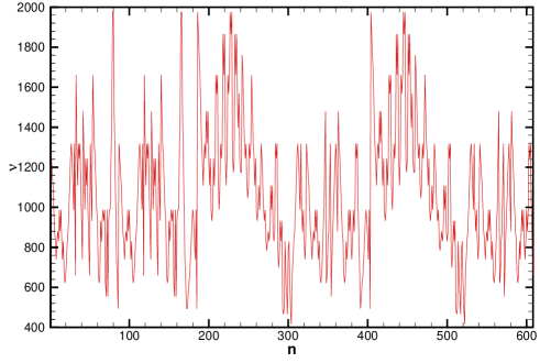
Figure 1: Typical up) sheet music and down) frequency series of Invention No.6 by Bach.

We use DFA method for the analysis and elimination of trends from data sets. DFA method introduced by Peng et al. Peng94 has became a widely used technique for the determination of (mono-) fractal scaling properties and the detection of long-range correlations in noisy, non-stationary time series physa ; kunhu . It has successfully been applied to diverse fields such as DNA sequences Peng94 ; DNA , cardiac dynamics cardiac , climate climate , neural receptors nural , economical time series economics etc.

The paper is organized as follows: In section II we describe DFA methods in details and analyze the frequency series of the Inventions and Sinfonias. We end the paper by drawing conclusions.

2 DFA and analysis of music frequency series

To implement the DFA, let us suppose we have a time series, $N(i)(i=1,...,N_{max})$ and determine the profile: $y(j)=\sum_{i=1}^{j}[N(i)-\langle N\rangle]$. Next we break up $N(i)$ into $K$ non-overlapping time intervals, $I_{n}$, of equal size $\tau$ where $n=0,1,...K-1$ and $K$ corresponds to the integer part of $N_{max}/\tau$. In each box, we fit the integrated time series by using a polynomial function, $y_{pol}(i)$, which is called the local trend. We detrend the integrated time series $y(i)$ in each box, and calculate the detrended fluctuation function: $Y(i)=y(i)-y_{pol}(i)$. For a given box size $s$, we calculate the root mean square fluctuation:

$$F(s)=\sqrt{\frac{1}{N_{max}}\sum_{i=1}^{N_{max}}[Y(i)]^{2}}.$$ (1)

The above computation is repeated for box sizes $s$ (different scales) to provide a relationship between $F(s)$ and $s$. A power law relation between $F(s)$ and $s$ indicates the presence of scaling

$$F(s)\sim s^{H}.$$ (2)

The parameter $H$, called Hurst exponent, represents the correlation properties of the signal: if $H=0.5$, there is no correlation and the signal is an uncorrelated signal Peng94 ; if $H<0.5$, the signal is anticorrelated; if $H>0.5$, there are positive correlations in the signal. In the two latest cases, the signal can be well approximated by the fractional Brownian motion law Feder88 . Also, the auto correlation function can be characterized by a power law $C(s)\equiv\langle N_{k}N_{k+s}\rangle\sim s^{-\gamma}$ with $\gamma=2-2H$. Its power spectra can be characterized by $S(\omega)\sim\omega^{-\beta}$ with frequency $\omega$ and $\beta=2H-1$. In non-stationary case, correlation exponent and power spectrum scaling are $\gamma=-2H$ and $\beta=2H+1$, respectively Peng94 ; eke02 .

It can be checked out that, frequency series is non-stationary. One can verify non-stationarity properties experimentally by measuring stability of average and variance in moving windows by, for example, using scale $s$ (Fig. 2a).

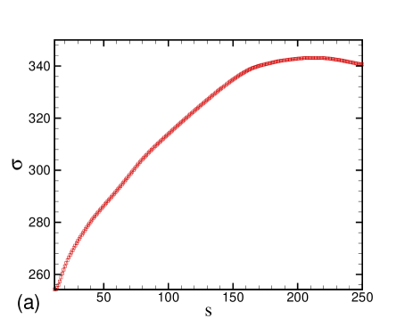
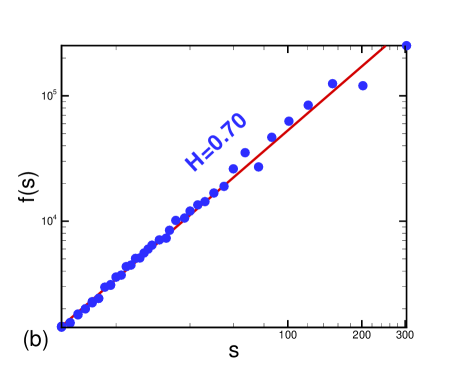
Figure 2: a) $s$ dependence of variation and b) The log-log plot $F(s)$ versus $s$ for Invention no.6 frequency series.

In Fig. 2b we plot in double-logarithmic scale the corresponding fluctuation function $F(s)$ against the box size s. Using the above procedure, we obtain the following estimate for the Hurst exponent: $H=0.70\pm 0.03$. The $F(s)$ exhibits an approximate scaling regime from $s=2$ up to nearly $s=6$ (in logarithmic scale). Since $H>0.5$ it is concluded that the frequency series show persistence; i.e. strong correlations between consecutive increments. The values which derived for quantities of DFA1 method for Invention no. 6 are given in Table 1 (second line). We have calculated the Hurst exponent for other Inventions and Sinfonia as well, all being in the $0.7-0.8$ range (Table 1).

Usually, in DFA method, deviation from a straight line in log-log plot of Eq.(2) occurs for small scales $s$. These deviations are intrinsic to the usual DFA method, since the scaling behavior is only approached asymptotically. Deviations limit the capability of DFA to determine the correct correlation behavior in very short records and in the regime of small $s$. The modified DFA is defined as follows physa :

$$F^{\rm mod}(s) = F(s){\langle[F^{\rm shuf}(s^{\prime})]^{2}\rangle^{1/2}\,s^{1/2}\over\langle[F^{\rm shuf}(s)]^{2}\rangle^{1/2}\,s^{\prime 1/2}}\quad{\rm(for}\,\,\,s^{\prime}\gg 1),$$ (3)

where $\langle[F^{\rm shuf}(s)]^{2}\rangle^{1/2}$ denotes the usual DFA fluctuation function, defined in Eq.(1), averaged over several configurations of shuffled data taken from original series, and $s^{\prime}\approx N/20$. The improvement is very useful especially for short records or records that have to be split into shorter parts to eliminate problematic nonstationarities, since the small $s$ regime can be included in the fitting range for the fluctuation exponent $H$.

The modified DFA method indicates the correct correlation behavior also in presence of broadly distributed data, where the common DFA fails to distinguish long-range correlations from deviations caused by broad distributions. The values of Hurst exponent obtained by modified DFA1 methods for frequency series is $0.72\pm 0.03$. The relative deviation of Hurst exponent which is obtained by modified DFA1 in comparison to DFA1 for original data is less than $4\%$.

Table 1: Values of Hurst $(H)$, power spectrum scaling $(\beta)$ and auto-correlation scaling $(\gamma)$ exponents for the selections of Inventions and sinfonias frequency series obtained by DFA1.

	$H$	$\beta$	$\gamma$
Invention no.1	$0.77\pm 0.03$	$2.54\pm 0.06$	$-1.54\pm 0.03$
Invention no.6	$0.72\pm 0.03$	$2.44\pm 0.06$	$-1.44\pm 0.03$
Sinfonia no.1	$0.71\pm 0.03$	$2.42\pm 0.06$	$-1.42\pm 0.03$
Sinfonia no.13	$0.73\pm 0.03$	$2.46\pm 0.06$	$-1.46\pm 0.03$

3 Conclusion

DFA is a scaling analysis method used to quantify long-range power-law correlations in signals. Many physical and biological signals are ‘noisy’, heterogeneous and exhibit different types of nonstationarities, which can affect the correlation properties of these signals. Applying DFA1 method demonstrates that the music frequency series have long range correlation. We calculated Hurst exponent for other Inventions and Sinfonia and found it to be in the $0.7-0.8$ range.

4 Acknowledgment

GRJ would like to acknowledge the hospitality extended during his visit at the IPM, UCLA, where this work was started.

References

- (1) D.L. Gonzalez, L. Morettini, F. Sportolari, O. Rosso, J.H.E. Cartwright and O. Piro, arXiv:chao-dyn/9505001, (1995).
- (2) Julyan H. E. Cartwright, Diego L. Gonz alez, and Oreste Piro, 1999 Phys. Rev. Lett. 82, 5389.
- (3) Heather D. Jennings, Plamen Ch. Ivanov, Allan de M. Martins, P.C. da Silva, G.M. Viswanathan, Physica A 336 (2004) 585 594.
- (4) Jean Pierre Boon and Olivier Decroly, 1995, Chaos 5(3) 501-508.
- (5) Rudi Cilibrasi, Paul Vitanyi and Ronald de Wolf, Computer Music Journal, 28:4, pp. 49 67, Winter 2004; Rudi Cilibrasi and Paul Vitanyi, 2005, IEEE TRANSACTIONS ON INFORMATION THEORY, 51(4), 1523 1545.
- (6) Peng C K, Buldyrev S V, Havlin S, Simons M, Stanley H E, and Goldberger A L, 1994 Phys. Rev. E 49, 1685; G. M. Viswanatha, C.-K. Peng, H. E. Stanley, and A. L. Goldberger, Phys. Rev. E 55, 845 (1997).
- (7) Hurst H E, Black R P and Simaika Y M, 1965 Long-term storage. An experimental study (Constable, London).
- (8) Muzy J F, Bacry E and Arneodo A, 1991 Phys. Rev. Lett. 67, 3515
- (9) Kantelhardt J W, Koscielny-Bunde E, Rego H H A, Havlin S and Bunde A, 2001 Physica A 295, 441.
- (10) Hu K, Ivanov P Ch, Chen Z, Carpena P and Stanley H E, 2001 Phys. Rev. E 64, 011114.
- (11) C.-K. Peng, S.V. Buldyrev, A.L. Goldberger, S. Havlin, F. Sciortino, M. Simons, and H.E. Stanley, Nature (Lon- don) 356, 168 (1992); R.N. Mantegna, S.V. Buldyrev, A.L. Goldberger, S. Havlin, C.-K. Peng, M. Simons, and H.E. Stanley, Phys. Rev. Lett. 73, 3169 (1994); R.N. Mantegna, S.V. Buldyrev, A.L. Goldberger, S. Havlin, C.-K. Peng, M. Simons, and H.E. Stanley, Phys. Rev. Lett. 76, 1979 (1996).
- (12) P.Ch. Ivanov, M.G. Rosenblum, C.-K. Peng, J.E. Mietus, S. Havlin, H.E. Stanley, and A.L. Goldberger, Nature (London) 383, 323 (1996); Ashkenazy Y, Ivanov P Ch, Havlin S, Peng C K, Goldberger A L and Stanley H E, 2001 Phys. Rev. Lett. 86, 1900; Bunde A, Havlin S, Kantelhardt J W, Penzel T, Peter J H and Voigt K, 2000 Phys. Rev. Lett. 85, 3736.
- (13) Koscielny-Bunde E, Bunde A, Havlin S, Roman H E, Goldreich Y and Schellnhuber H J, 1998 Phys. Rev. Lett. 81, 729; Ivanova K, Ausloos M, Clothiaux E E and Ackerman T P, 2000 Europhys. Lett. 52, 40.
- (14) S. Bahar, J.W. Kantelhardt, A. Neiman, H.H.A. Rego, D.F. Russell, L. Wilkens, A. Bunde, and F. Moss, Euro- phys. Lett. 56, 454 (2001).
- (15) N. Vandewalle and M. Ausloos, Phy. Rev. E 58, 6832 (1998); P. Grau-Carles, Physica A 287, 396 (2000).
- (16) Feder J, 1988 Fractals (Plenum Press, New York)
- (17) Eke A, Herman P, Kocsis L and Kozak L R, 2002 Physiol. Meas. 23, R1-R38.