On the Definition of Effective Permittivity and Permeability For Thin Composite Layers

Abstract

The problem of definition of effective material parameters (permittivity and permeability) for composite layers containing only one-two parallel arrays of complex-shaped inclusions is discussed. Such structures are of high importance for the design of novel metamaterials, where the realizable layers quite often have only one or two layers of particles across the sample thickness. Effective parameters which describe the averaged induced polarizations are introduced. As an explicit example, we develop an analytical model suitable for calculation of the effective material parameters $\varepsilon_{\rm{eff}}$ and $\mu_{\rm{eff}}$ for double arrays of electrically small electrically polarizable scatterers. Electric and magnetic dipole moments induced in the structure and the corresponding reflection and transmission coefficients are calculated using the local field approach for the normal plane-wave incidence, and effective parameters are introduced through the averaged fields and polarizations. In the absence of losses both material parameters are purely real and satisfy the Kramers-Kronig relations and the second law of thermodynamics. We compare the analytical results to the simulated and experimental results available in the literature. The physical meaning of the introduced parameters is discussed in detail.

I Introduction

The problem of extraction of material parameters for composite slabs implemented using complex-shape inclusions (often referred to as metamaterial slabs) has been discussed in a large number of recent articles, see e.g. [1, 2, 3, 4, 5, 6, 7, 8, 9, 10] for some example contributions. The physical meaning of many of the recent retrieval results is, however, controversial. Typically, the $S$-parameter retrieval procedure based on the Fresnel formulae is used to extract the effective material parameters under the normal plane-wave incidence. This technique is often known to lead to nonphysical material parameters that violate the second law of thermodynamics: Either the real part of $\varepsilon_{\textrm{eff}}$ or $\mu_{\textrm{eff}}$ obeys antiresonance and therefore the corresponding imaginary part has a “wrong” sign, see [3, 7] for some results indicating this phenomenon, and [4, 5, 6] for related criticism. It is important to bear in mind that even though the aforementioned material parameters might satisfy the Kramers-Kroning relations (thus being causal), these parameters have no physical meaning in electromagnetic sense as physically meaningful material parameters must satisfy simultaneously both the causality requirement and the passivity requirement [11]. The above discussed parameters (from now on we do not use for them the term “material parameter”) allow, however, to correctly reproduce the scattering results for normal plane wave incidence.

One particular example of complex slabs, referred to in the beginning of the paper, is double arrays of small scatterers. Such slabs present a very interesting problem as in several recent papers the authors state that double grids of electrically short wires (or electrically small plates) can be used to produce negative index of refraction in the optical [12, 13, 14, 15] and in the microwave regime [16]. In some cases, however, the nonphysical (antiresonant) behavior is seen in the extracted material parameters [14, 16] casting doubts over the meaningfulness of assigning negative index of refraction for these structures.

The goal of this work is to formulate the effective material parameters for double arrays of small scatterers through the macroscopic polarization and magnetization, and compare the results to those obtained using the $S$-parameter retrieval method (the reference results are obtained by different authors [14]). The particles in the arrays are modeled as electrically small electric dipoles in order to calculate, by using the local field approach, currents induced to each of the particles at normal plane wave incidence. Knowing the induced currents, the reflection and transmission coefficients for the arrays, as well as the induced electric and magnetic dipole moment densities (macroscopic polarization and magnetization) are calculated. Effective material parameters are then defined directly using the expressions for the averaged fields and the macroscopic polarization and magnetization. Finally, the double array is represented as a slab of a homogeneous material characterized by effective material parameters.

Since the layer is electrically thin and spatially dispersive, it is obvious that an effective material parameter model cannot adequately and fully describe the layer’s electromagnetic properties, and, moreover, effective parameters can be introduced in different ways. It is important to understand the physical meaning of different effective medium models and their applicability regions. In this paper we compare the material parameter extraction based on macroscopic properties calculated by means of the local field approach with the conventional method based on the $S$-parameter inversion.

The paper is organized in the following way: In Section II we use the local field approach to calculate the electric dipole moments induced in the particles and define the averaged fields needed in the determination of the effective material parameters. The derivation of these parameters is presented in Section III. In Section IV some calculated example results are presented, and these results are qualitatively compared with the numerical and experimental results available in the literature. Discussion is conducted on the physics behind the results. The work is concluded in Section V.

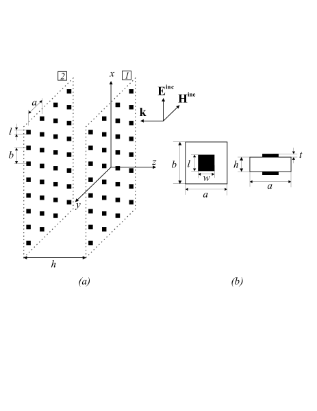
Figure 1: (a) Geometry of a double array of small scatterers (square patches). (b) The unit cell.

II Local field approach to determine the dipole moments and the averaged fields

II-A Electric dipole moments induced in the particles

Consider a double array of scatterers shown in Fig. 1. At this point the shape of the particles can be arbitrary, provided that they can be modeled using the electric dipole approximation. With this assumption the response of each particle can be described in terms of the induced electric dipole moment p which is determined by the particle polarizability $\alpha$ and the local electric field at the particle position.

The array is excited by a normally incident plane expressed as (see Fig. 1(a))

$$\mathbf{E}^{\rm ext}=\mathbf{E}_{0}e^{jk_{0}z}=E_{0}\mathbf{x}e^{jk_{0}z}.$$ (1)

The common notation for the wavenumber $k_{0}=\omega\sqrt{\varepsilon_{0}\mu_{0}}$ and for the free-space wave impedance $\eta_{0}=\sqrt{\mu_{0}/\varepsilon_{0}}$ is used. The electric dipole moment induced in a reference particle sitting in the first and the second grids reads:

$$\mathbf{p}_{1,2}=\alpha_{1,2}\mathbf{E}_{1,2}^{\rm loc},$$ (2)

where $\mathbf{E}_{1,2}^{\rm loc}$ is the local electric field exciting the reference particles. Since both layers are identical in this analysis, the notation for the particle polarizability is simplified as $\alpha_{1}=\alpha_{2}=\alpha$. The local electric fields can be expressed as

$$\mathbf{E}_{1}^{\rm loc}=\mathbf{E}_{1}^{\rm ext}+\beta(0)\mathbf{p}_{1}+\beta(h)\mathbf{p}_{2},$$

$$\mathbf{E}_{2}^{\rm loc}=\mathbf{E}_{2}^{\rm ext}+\beta(h)\mathbf{p}_{1}+\beta(0)\mathbf{p}_{2},$$ (3)

where $\beta(0)$ is called the self-interaction coefficient and $\beta(h)$ is the mutual interaction coefficient. Physically, $\beta(0)$ takes into account the contribution to the local field of the particles located in the same grid as the reference particle, whereas $\beta(h)$ takes into account the influence of the other grid.

By combining Eqs. (1), (2) and (3), the following system of equations is obtained for the unknown dipole moments:

$$\alpha^{-1}\mathbf{p}_{1}=\mathbf{E}_{0}+\beta(0)\mathbf{p}_{1}+\beta(h)\mathbf{p}_{2},$$

$$\alpha^{-1}\mathbf{p}_{2}=\mathbf{E}_{0}e^{-jk_{0}h}+\beta(h)\mathbf{p}_{1}+\beta(0)\mathbf{p}_{2}.$$ (4)

Solving this system of equations, the electric dipole moments induced on the particles in layers 1 and 2 read:

$$\mathbf{p}_{1}=\frac{\mathbf{E}_{0}}{\Delta}\bigg{[}\alpha^{-1}-\beta(0)+\beta(h)e^{-jk_{0}h}\bigg{]},$$ (5)

$$\mathbf{p}_{2}=\frac{\mathbf{E}_{0}}{\Delta}\bigg{[}[\alpha^{-1}-\beta(0)]e^{-jk_{0}h}+\beta(h)\bigg{]},$$ (6)

where $\Delta=[\alpha^{-1}-\beta(0)]^{2}-\beta(h)^{2}$. Approximate analytical formulas for the interaction coefficients have been established in [17, 18, 19, 20]:

$$\beta(0)=-\textrm{Re}\bigg{[}\frac{j\omega\eta_{0}}{4S_{0}}\bigg{(}1-\frac{1}{jk_{0}R}\bigg{)}e^{-jk_{0}R}\bigg{]}+\\ +j\bigg{(}\frac{k_{0}^{3}}{6\pi\varepsilon_{0}}-\frac{\eta_{0}\omega}{2S_{0}}\bigg{)},$$ (7)

$$\beta(h)=-\textrm{Re}\bigg{[}\frac{j\omega\eta_{0}}{4S_{0}}\bigg{\{}1-\frac{1}{jk_{0}\sqrt{R^{2}+h^{2}}}+\\ +\frac{h^{2}}{R^{2}+h^{2}}\bigg{(}1+\frac{1}{jk_{0}\sqrt{R^{2}+h^{2}}}\bigg{)}\bigg{\}}e^{-jk_{0}\sqrt{R^{2}+h^{2}}}+\\ +\frac{1}{4\pi\varepsilon_{0}}\bigg{\{}\frac{1}{h^{3}}+\frac{jk_{0}}{h^{2}}-\frac{k_{0}^{2}}{h}e^{-jk_{0}h}\bigg{]}+\\ -j\frac{\eta_{0}\omega}{2S_{0}}\cos(k_{0}h),$$ (8)

where $S_{0}$ is the unit cell area (for the rectangular-cell array $S_{0}=a\times b$, Fig. 1(b), and parameter $R$ is equal to $a/1.438$ [18]). The imaginary parts of the interaction constants $\beta(0)$ and $\beta(h)$ are exact, so that the energy conservation law is satisfied. The real parts are approximate, and the model is rather accurate for $ka<1.5\dots 2$ [18, 19, 20]. Note that the present definition of polarizability $\alpha$ includes also the effects of scattering, thus remaining a complex number even in the absence of absorption. If there is no absorption in the particles, the imaginary part of $\alpha$ reads (e.g., [21]):

$$\textrm{Im}\bigg{\{}\frac{1}{\alpha}\bigg{\}}=\frac{\eta_{0}\varepsilon_{0}\mu_{0}\omega^{3}}{6\pi}=\frac{k_{0}^{3}}{6\pi\varepsilon_{0}}.$$ (9)

In the far zone, the reflected field of one grid is a plane wave field with the amplitude [21]

$$\mathbf{E}^{\rm ref}_{1,2}=-j\frac{\eta_{0}\omega}{2S_{0}}\mathbf{p}_{1,2}.$$ (10)

The scattered plane-wave field at the reference plane $z=0$ reads:

$$\mathbf{E}^{\rm ref}_{z=0}=\mathbf{E}_{1}^{\rm ref}+\mathbf{E}_{2}^{\rm ref}=-j\frac{\eta_{0}\omega}{2S_{0}}(\mathbf{p}_{1}+\mathbf{p}_{2}e^{-jk_{0}h}).$$ (11)

Finally, the reflection and transmission coefficients can be written as:

$$R=\frac{E^{\rm ref}}{E^{\rm inc}}\bigg{|}_{z=0}=-j\frac{\eta_{0}\omega}{2S_{0}E_{0}}(p_{1}+p_{2}e^{-jk_{0}h}),$$ (12)

$$T=\frac{E^{\rm trans}}{E^{\rm inc}}\bigg{|}_{z=0}=1-j\frac{\eta_{0}\omega}{2S_{0}E_{0}}(p_{1}+p_{2}e^{jk_{0}h}).$$ (13)

II-B Definition of the averaged fields

The total averaged electric and magnetic fields in the vicinity of the array are, by definition, the sum of incident field and the averaged scattered field:

$$\widehat{\mathbf{E}}=\langle\mathbf{E}^{\rm inc}+\mathbf{E}^{\rm ref}\rangle,\quad\widehat{\mathbf{H}}=\langle\mathbf{H}^{\rm inc}+\mathbf{H}^{\rm ref}\rangle.$$ (14)

Under plane-wave excitation each grid creates reflected and transmitted plane waves having the amplitudes given by Eq. (10). Those fields are the scattered fields averaged in the transverse plane. In order to average the fields inside the slab, the field that is scattered by the first grid and propagates towards the second grid, and the field scattered by the second grid and propagating towards the first grid are considered, see Fig. 2.

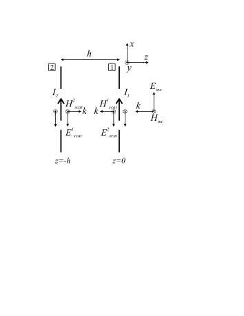
Figure 2: Incident and scattered fields in the problem geometry.

The averaged electric field inside the slab can be expressed as follows:

$$\widehat{\mathbf{E}}=\frac{1}{h}\int_{-h}^{0}\bigg{[}\mathbf{E}_{0}e^{jk_{0}z}-j\frac{\eta_{0}\omega}{2S_{0}}\bigg{(}\mathbf{p}_{1}e^{jk_{0}z}+\mathbf{p}_{2}e^{-jk_{0}(z+h)}\bigg{)}\bigg{]}dz.$$ (15)

After conducting the integration, we find the volume-averaged electric field:

$$\widehat{\mathbf{E}}=e^{-jk_{0}h/2}\bigg{(}\mathbf{E}_{0}-j\frac{\eta_{0}\omega}{2S_{0}}(\mathbf{p}_{1}+\mathbf{p}_{2})\bigg{)}\frac{\sin(k_{0}h/2)}{k_{0}h/2}.$$ (16)

Analogously, the averaged magnetic field can be expressed as

$$\widehat{\mathbf{H}}=-\frac{e^{-jk_{0}h/2}}{\eta_{0}}\bigg{(}\mathbf{E}_{0}-j\frac{\eta_{0}\omega}{2S_{0}}(\mathbf{p}_{1}-\mathbf{p}_{2})\bigg{)}\frac{\sin(k_{0}h/2)}{k_{0}h/2}.$$ (17)

III Effective material parameters

Let us start from the common definition of the constitutive parameters of an isotropic homogeneous material:

$$\mathbf{D}=\varepsilon_{0}\widehat{\mathbf{E}}+\mathbf{P}=\varepsilon_{0}\varepsilon_{\textrm{eff}}\widehat{\mathbf{E}},\quad\mathbf{P}=\frac{\mathbf{p}}{V},$$ (18)

$$\mathbf{B}=\mu_{0}\widehat{\mathbf{H}}+\mathbf{M}=\mu_{0}\mu_{\textrm{eff}}\widehat{\mathbf{H}},\quad\mathbf{M}=\frac{\mathbf{m}}{V}.$$ (19)

Here $\mathbf{P}$ and $\mathbf{M}$ are the volume-averaged polarization and magnetization, $\mathbf{p}$ and $\mathbf{m}$ are the electric and magnetic dipole moments induced in the unit cell, and $V$ is the volume of the unit cell. Knowing $\widehat{\mathbf{E}}$, $\widehat{\mathbf{H}}$, $\mathbf{P}$, and $\mathbf{M}$ for our particular layer we define effective material parameters as:

$$\varepsilon_{\textrm{eff}}=1+\frac{\mathbf{P}}{\varepsilon_{0}\widehat{\mathbf{E}}},\quad\mu_{\textrm{eff}}=1+\frac{\mathbf{M}}{\mu_{0}\widehat{\mathbf{H}}}.$$ (20)

Naturally, these parameters have more limited physical meaning than the usual parameters of a bulk homogeneous sample, but they can be used as a measure for averaged polarizations in a thin layer. Let us next find these parameters for our particular example grid in terms of its geometry and inclusion polarizabilities.

In order to simplify the forthcoming notations, the sum and difference of the electric dipole moments with the use of Eqs. (5), (6) can be written in the following manner:

$$\mathbf{p_{1}}+\mathbf{p_{2}}=\mathbf{E}_{0}\frac{2e^{-jk_{0}h/2}\cos(k_{0}h/2)}{\alpha^{\prime-1}},$$ (21)

$$\mathbf{p_{1}}-\mathbf{p_{2}}=\mathbf{E}_{0}\frac{2je^{-jk_{0}h/2}\sin(k_{0}h/2)}{\alpha^{\prime\prime-1},}$$ (22)

where

$$\alpha^{\prime-1}=\alpha^{-1}-\beta(0)-\beta(h),$$ (23)

$$\alpha^{\prime\prime-1}=\alpha^{-1}-\beta(0)+\beta(h).$$ (24)

It is important to note that for lossless particles the imaginary parts of $\alpha^{\prime-1}$ and $\alpha^{\prime\prime-1}$ can be solved exactly from the power balance requirement [19]:

$$\textrm{Im}\{\alpha^{\prime-1}\}=\frac{\eta_{0}\omega}{S_{0}}\cos^{2}(k_{0}h/2),$$ (25)

$$\textrm{Im}\{\alpha^{\prime\prime-1}\}=\frac{\eta_{0}\omega}{S_{0}}\sin^{2}(k_{0}h/2).$$ (26)

The use of exact expressions for the imaginary parts is very important: Approximate relations would lead to complex material parameters of lossless grids, where the imaginary part would have no physical meaning.

The total averaged electric polarization which we need to substitute in Eq. (20) reads

$$\mathbf{P}=\frac{\mathbf{p}_{1}+\mathbf{p}_{2}}{V}.$$ (27)

In the following, we consider lossless particles with the inverse polarizabilities

$$\alpha^{\prime-1}={\rm{Re}}\{\alpha^{\prime-1}\}+j{\rm{Im}}\{\alpha^{\prime-1}\},$$ (28)

$$\alpha^{\prime\prime-1}={\rm{Re}}\{\alpha^{\prime\prime-1}\}+j{\rm{Im}}\{\alpha^{\prime\prime-1}\}.$$ (29)

The imaginary parts in the above relations satisfy (25) and (26). Substituting first (21) into (27), and then (27) into (20), the effective permittivity obtained after some mathematical manipulations is as follows:

$$\varepsilon_{\textrm{eff}}=1+\frac{k_{0}h}{V\varepsilon_{0}}\bigg{[}\textrm{Re}\{\alpha^{\prime-1}\}\tan\bigg{(}\frac{k_{0}h}{2}\bigg{)}-\frac{\eta_{0}\omega}{S_{0}}\sin^{2}\bigg{(}\frac{k_{0}h}{2}\bigg{)}\bigg{]}^{-1}.$$ (30)

Notice that the permittivity is purely real, as it should be since the particles in the arrays are lossless.

For our system of two identical grids of small particles the effective permeability $\mu_{\textrm{eff}}$ defined by (20) can be also expressed in terms of the induced electric dipole moments. Considering one unit cell formed by two particles of length $l$ with $x$-directed dipole moments $p_{1,2}$, we can write for the currents on the particles (averaged along $x$) $I_{1,2}=j\omega p_{1,2}/l$. The magnetic moment of this pair of particles (referred to the unit cell center) is then

$$m=\mu_{0}l\frac{h}{2}(I_{1}-I_{2})=j\omega\mu_{0}\frac{h}{2}(p_{1}-p_{2}).$$ (31)

After inserting first (22) into (31), and then (31) into (20), the effective permeability reads:

$$\mu_{\textrm{eff}}=1+\frac{\eta_{0}\omega k_{0}h^{2}}{2V}\bigg{[}\textrm{Re}\{\alpha^{\prime\prime-1}\}+\frac{\eta_{0}\omega}{2S_{0}}\sin(k_{0}h)\bigg{]}^{-1}.$$ (32)

We can again observe that this quantity is purely real, as it should be in the absence of losses. Notice that the procedure presented here can easily be generalized to different particle geometries.

As is apparent from the definition, these effective parameters measure cell-averaged electric and magnetic polarizations in the layer. Can they be used to calculate the reflection and transmission coefficients from the layer? This question will be considered next using a numerical example.

IV Numerical examples

In this section, the double array of square patches studied in [14] is considered as a representative example of comparison between the effective parameters introduced here and material parameters formally extracted from measured or calculated $S$-parameters.

The geometry of the double-grid array is the same as considered above (Fig. 1). The unit cell is characterized by the following parameters: Edge lengths of the patches $t=l$, the lattice constants $a=b$, the metal layer thickness $p$, and the distance between the layers equals $h$. The dimensions of the unit cell considered in [14] are the following: $w=l=300$ nm, $t=20$ nm, $a=b=650$ nm, $p=20$ nm, $h=80$ nm. Since the double array considered in [14] is targeted to the use at THz frequencies, the metal thickness $p$ becomes comparable to the dielectric spacer thickness $h$. The physical thickness of the slab is $D=h+2p$. However, at THz frequencies one must take into account nonzero fields inside metal particles (here gold is considered, which at these high frequencies is usually characterized by the Drude model (e.g., [11])). For this reason an effective thickness of $D_{\rm eff}=1.5D$ is chosen for the analysis, but we should bear in mind that this is only a rough estimation, and an accurate determination of this effective slab thickness is very difficult.

Notice that, as it is stated in [20], the limitation $ka<1.5...2$ in the analytical model for the interaction constants (Section II) is not critical for these calculations until the lattice resonance at $ka=2\pi$ is reached, since the reflection properties near resonances are mainly determined by the particle resonances. In this case, it means that the model is accurate enough up to approximately 460 THz.

The following rough estimates are used for calculating the particle polarizabilities. A known [21] antenna model for short strip particles is used by setting the particle width equal to the particle length. The polarizability is resonant and can be characterized in the microwave regime by an equivalent LC-circuit, where $C$ is approximated as the input capacitance of a small dipole antenna having length $l$ and radius $r_{0}=w/4$, and $L$ is the inductance of a short strip having length $l$, width $w$, and thickness $t$ [22]:

$$C\approx\frac{\pi(l/2)\varepsilon_{0}}{\log(l/r_{0})},$$ (33)

$$L\approx 0.2l\bigg{(}\log\frac{l}{w+t}+1.19+0.22\frac{w+t}{l}\bigg{)}.$$ (34)

(The values of $l,w,t$ are inserted in eq. (34) in millimeters. The result is in nano-Henrys.) As mentioned above, in the THz range the behavior of metals is different from the microwave regime. Following the treatment in [23], the penetration of fields inside the particles can be represented by an additional parallel capacitance $C_{\textrm{add}}$ and a series inductance $L_{\textrm{add}}$ [23]:

$$C_{\textrm{add}}=\frac{\varepsilon_{0}wt}{l_{\textrm{eff}}},$$ (35)

$$L_{\textrm{add}}=\frac{l_{\textrm{eff}}}{\varepsilon_{0}wt\omega_{p}^{2}},$$ (36)

where $\omega_{p}$ is the plasma frequency of considered metal (gold in this case) and $l_{\textrm{eff}}$ is the effective particle length. The physical clarification of the above parameters is available in [23]. Due to the cosine current distribution the effective length is approximated as $l_{\textrm{eff}}=2l$. Finally, the particle polarizability reads:

$$\alpha=\frac{(C+C_{\textrm{add}})l^{2}}{1-\omega^{2}(L+L_{\textrm{add}})(C+C_{\textrm{add}})}$$ (37)

Fig. 3 shows the magnitudes of the reflection and transmission coefficients calculated using Eqs. (12) and (13). Comparing this result with the experimental results presented in Fig. 4a of Ref. [14], good agreement is observed. The shape of the reflection and transmission functions follows the ones presented in [14]. The differences in the amplitude levels and transmission frequencies are well expected: The model used here does not take losses in the particles into account.

Figure 3: Calculated reflection and transmission coefficients.

The effective material parameters calculated using Eqs. (30) and (32) are depicted in Fig. 4. Both material parameters clearly behave in a physically sound manner: They are purely real, since lossless particles have been considered, and they are growing functions outside the resonant region. Contrary, the material parameters extracted in [14] for the same structure behave in a nonphysical manner: The imaginary parts of permittivity and permeability have the opposite signs over certain frequency ranges, thus, the passivity requirement is violated [4, 5, 11]. It is evident also from Fig. 4c and 4d of Ref. [14] that the extracted material parameters do not satisfy the Kramers-Kronig relations (e.g., the antiresonance in the real part of permittivity cannot correspond to a positive imaginary part (with the authors’ time dependence assumption) if inserted into Kramers-Kronig relations), thus, they have quite limited physical meaning [11]. Both of these problems are avoided with the method described here. On the other hand, the material parameters extracted from the reflection and transmission coefficients reproduce these properties of the layer exactly, while the parameters introduced here do not necessarily give so accurate predictions for reflection and transmission coefficients.

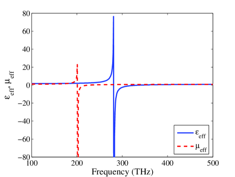
Figure 4: Calculated effective permittivity and permeability.

This is illustrated next by representing the double layer of particles as a slab of a homogeneous material having thickness $D_{\rm eff}$ and characterized by the material parameters shown in Fig. 4. The standard transmission-line equations are used to calculate the reflection and transmission coefficients for a normally incident plane wave. The result is depicted in Fig. 5. When comparing Figs. 3 and 5 it can be observed that the results do not correspond exactly to each other, even thought the principal features such as reflection frequencies around 200 and 300 THz seen in Fig. 3 are reproduced in Fig. 5. This is an expected result: There is no such uniform material (with physically sound material parameters) that would behave exactly as the actual double grid of resonant particles. In a truly homogeneous material the unit cell over which the averaging is performed should contain a large number of “molecules” yet remaining small compared to the wavelength. It is clear that for the considered double array this is not the case, and also spatial dispersion effects cannot be neglected.

In particular, very close to the grid resonances the induced dipole moments are very large, which corresponds to large values of the present effective parameters and to large electrical thickness of the homogenized slab. These large values correctly describe large polarizations in the grids, but they fail to correctly predict the reflection and transmission coefficients. On the contrary, the effective parameters retrieved from the layer’s $S$- parameters, correctly describe these reflection and transmission coefficients, but they do not describe polarization properties of the actual structure.

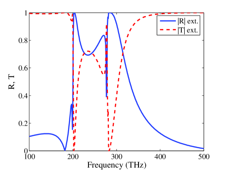
Figure 5: Reflection and transmission coefficients calculated when the double array is represented as a slab of homogeneous material characterized by $\varepsilon_{\textrm{eff}},\mu_{\textrm{eff}}$ depicted in Fig. 4.

It is also important to note that the standard $S$-parameter retrieval procedure often leads to nonphysical material parameters (see the discussion above). The material parameters defined through macroscopic polarization and magnetization are always physically sound since they are defined directly by the actual dipole moments induced in the microstructure. Thus, the effective material parameters assigned in this way always make physical sense.

V Conclusion

In this paper an analytical model to assign effective material parameters $\varepsilon_{\textrm{eff}}$ and $\mu_{\textrm{eff}}$ for double arrays of electrically small scatterers has been presented. The induced electric dipole moments have been calculated using the local field approach for a normally incident plane wave, and the corresponding averaged fields have been determined. The effective material parameters have been defined directly through the macroscopic polarization and magnetization. The derived expressions have been validated by comparing the calculations to the numerical and experimental results available in the literature. The main conclusion from this study is that simple effective medium models of electrically thin layers with complex internal structures are always limited in their applicability and in their physical meaning. Some models are best suitable to describe reflection and transmission coefficients at normal incidence (like the parameters conventionally retrieved from S-parameters), other models describe well the averaged induced polarizations in the structure and allow one to make conclusions about, for instance, negative permeability property (like the parameters introduced in this paper). In applications, it is important to understand what model is used and what properties of the layer this particular model actually describes. Finally, it is necessary to stress that the present study has been restricted to a particular special case of a dual layer of planar electrically polarizable particles. This approach needs appropriate modifications and extensions if, for instance, inclusions are also magnetically polarizable. For slabs containing more than two layers, the direct extension of this model corresponds to averaging over a unit cell containing three or more particles, which apparently is not useful for electrically thick slabs.

References

- [1] D. R. Smith, D. C. Vier, N. Kroll, and S. Schultz, “Direct calculation of permeability and permittivity for a left handed metamaterial”, Appl. Phys. Lett., vol. 77, no. 14, pp. 2246–2248, 2000.
- [2] D. R. Smith, S. Schultz, P. Markos, and C. M. Soukoulis, “Determination of effective permittivity and permeability of metamaterials from reflection and transmission coefficients”, Phys. Rev. B, vol. 65, pp. 195104(1–5), 2002.
- [3] T. Koschny, P. Markos, D. R. Smith, and C. M. Soukoulis, “Resonant and antiresonant frequency dependence of the effective parameters of metamaterials”, Phys. Rev. B, vol. 68, pp. 065602(1–4), 2003.
- [4] R. A. Delpine and A. Lakhtakia, “Comment I on “Resonant and antiresonant frequency dependence of the effective parameters of metamaterials””, Phys. Rev. B, vol. 70, p. 048601, 2004.
- [5] A. L. Efros, “Comment II on “Resonant and antiresonant frequency dependence of the effective parameters of metamaterials””, Phys. Rev. B, vol. 70, pp. 048602(1–2), 2004.
- [6] T. Koschny, P. Markos, D. R. Smith, and C. M. Soukoulis, “Reply to comments on “Resonant and antiresonant frequency dependence of the effective parameters of metamaterials””, Phys. Rev. B, vol. 70, p. 048603, 2004.
- [7] D. R. Smith, D. C. Vier, Th. Koschny, and C. M. Soukoulis, “Electromagnetic parameter retrieval from inhomogeneous metamaterials”, Phys. Rev. E, vol. 71, pp. 036617(1–11), 2005.
- [8] X. Chen, T. Gregorczyk. B.-I. Wu, J. Pacheo Jr., and J. A. Kong, “Robust method to retrieve the constitutive effective parameters of metamaterials”, Phys. Rev. E, vol. 70, pp. 016608(1–7), 2004.
- [9] D. R. Smith and J. B. Pendry, “Homogenization of metamaterials by field averagind (invited paper)”, J. Opt. Soc. Am. B, vol. 23, no. 3, pp. 391–403, 2006.
- [10] D. R. Smith, S. Schuring, and J. J. Mock, “Characterization of a planar artificial magnetic metamaterial surface”, Phys. Rev. E, vol. 74, pp. 036604(1–5), 2006.
- [11] L. D. Landau, E. M. Lifshitz, and L. P. Pitaevskii, Electrodynamics of continuous media, Oxford: Butterworth Heinemann, 2nd ed., 1984.
- [12] V. A. Podolkiy, A. K. Sarychev, and V. M. Shalaev, “Plasmon modes and negative refraction in metal nanowire composites”, Optics Express, vol. 11, no. 7, pp. 735–745, 2003.
- [13] V. M. Shalaev, W. Cai, U. K. Chettiar, H. Yuan, A. K. Sarychev, V. P. Drachev, and A. V. Kildishev, “Negative index of refraction in optical metamaterials”, Optics Lett., vol. 30, no. 24, pp. 3356–3358, 2005.
- [14] G. Dolling, C. Enkrich, M. Wegener, J. F. Zhou, C. M. Soukoulis, and S. Linden, “Cut-wire pairs and plate pairs as magnetic atoms for optical metamaterials”, vol. 30, no. 23, pp. 3198–3200, 2005.
- [15] A. V. Kildishev, W. Cai, U. K. Chettiar, H. Yuan, A. K. Sarychev, V. P. Drachev, and V. M. Shalaev, “Negative refractive index in optics of metal-dielectric composites”, J. Opt. Soc. Am. B, vol. 23, no. 3, pp. 423–433, 2006.
- [16] J. Zhou, L. Zhang, G. Tuttle, Th. Koschny, and C. M. Soukoulis, “Negative index materials using simple short wire pairs”, Phys. Rev. B, vol. 73, pp. 041101(1–4), 2006.
- [17] V. V. Yatsenko and S. I. Maslovski, “Electromagnetic diffraction by double arrays of dipole scatterers”, Proc. Int. Seminar Day on Diffraction’99, (St. Petersburg), pp. 196–199, 1999.
- [18] S. I. Maslovski and S. A. Tretyakov, “Full-wave interaction field in two-dimensional arrays of dipole scatterers”, Int. J. Electron. Commun. (AEU), vol. 53, no. 3, pp. 135–139, 1999.
- [19] V. Yatsenko, S. Maslovski, and S. Tretyakov, “Electromagnetic interaction of parallel arrays of dipole scatterers”, Progress in Electromagnetics Research, PIER, vol. 25, pp. 285–307, 2000.
- [20] V. V. Yatsenko, S. I. Maslovski, S. A. Tretyakov, S. L. Prosvirnin, and S. Zouhdi, “Plane-wave reflection from double arrays of small magnetoelectric scatterers”, IEEE Trans. Antennas Propag. vol. 51, no. 1, pp. 2–13, 2003.
- [21] S. Tretyakov, Analytical modeling in applied electromagnetics, Norwood, MA: Artech House, 2003.
- [22] M. Caulton, “Lumped elements in microwave integrated circuits,” in Advances in microwaves, vol. 8 (L. Young, ed.), pp. 143- 202, New York: Academic Press, Inc., 1974.
- [23] S. A. Tretyakov, “On geometrical scaling of split-ring and double-bar resonators at optical frequencies,” Metamaterials, vol. 1, pp. 40 -43, 2007.