Single-Scattering Optical Tomography

Abstract

We consider the problem of optical tomographic imaging in the mesoscopic regime where the photon mean free path is of order of the system size. Within the accuracy of the single-scattering approximation to the radiative transport equation, we show that it is possible to recover the extinction coefficient of an inhomogeneous medium from angularly-resolved measurements. Applications to biomedical imaging are described and illustrated with numerical simulations.

I Introduction

There has been considerable recent interest in the development of experimental methods for three-dimensional optical imaging of biological systems. Applications range from imaging of optically-thin (by which we mean nearly transparent) cellular and sub-cellular structures to optically-thick systems at the whole organ level in which multiple scattering of light occurs. In optically-thin systems, confocal microscopy Wilson and optical coherence microscopy Izatt_1994 can be used to generate three-dimensional images by optical sectioning. Alternatively, computed imaging methods such as optical projection tomography (OPT) Sharpe_2002 or interferometric synthetic aperture microscopy (ISAM) Ralston_2006 ; Ralston_2007 may be employed to reconstruct three-dimensional images by inversion of a suitable integral equation. In the case of OPT, the effects of scattering are ignored and geometrical optics is used to describe the propagation of light. The sample structure is then recovered by inversion of a Radon transform which relates the extinction coefficient of the sample to the measured intensity of the optical field. In the case of ISAM, the effects of scattering are accounted for within the accuracy of the first Born approximation to the wave equation. An inverse scattering problem is then solved to recover the susceptibility of the sample from interferometric measurements of the cross-correlation function of the optical field.

In optically-thick systems, multiple scattering of the illuminating field creates a fundamental obstruction to image formation. If the medium is macroscopically large and weakly absorbing, only diffuse light is transmitted. By making use of the diffusion approximation (DA) to the radiative transport equation (RTE) and solving an appropriate inverse problem, the aforementioned difficulty may, to some extent, be overcome. This approach forms the basis of diffusion tomography which can be used to reconstruct images with sub-centimeter resolution of highly-scattering media such as the human breast Arridge_1999 . The relatively low quality of reconstructed images is due to severe ill-posedness of the inverse problem.

Despite significant recent progress in optical imaging of both optically thin and thick media, little has been done for imaging of systems of intermediate optical thickness. This represents the subject of this study. In radiative transport theory, such systems are referred to as mesoscopic, meaning that the photon mean free path (also known as the scattering length) is of order of the system size vanrossum_1999 . In the mesoscopic scattering regime, applications to biological systems include engineered tissues and semitransparent organisms such as zebra fish, animal embryos, or small-animal extremities. In this case, light exhibits sufficiently strong scattering so that the image reconstruction methods of computed tomography are not applicable, yet the detected light is not diffuse and the diffusion tomography can not be employed.

In mesoscopic systems, the DA does not hold and the RTE must be used to describe the propagation of light vanrossum_1999 . In this study, light transport in the mesoscopic regime is described by the first-order scattering approximation to the radiative transport equation. This enables the derivation of a relationship between the extinction coefficient of the medium and the single-scattered light intensity, which represents the basis for a novel three-dimensional optical imagining technique that we propose and refer to as single scattering optical tomography (SSOT). SSOT uses angularly-selective measurements of scattered light intensity to reconstruct the optical properties of macroscopically inhomogeneous media, assuming that the measured light is predominantly single-scattered. The image reconstruction problem of SSOT consists of inverting a generalization of the Radon transform in which the integral of the extinction coefficient along a broken ray (which corresponds to the path of a single-scattered photon) is related to the measured intensity.

Our results are remarkable is several regards. First, similar to the case of computed tomography, inversion of the broken-ray Radon transform is only mildly ill-posed. Second, the inverse problem of the SSOT is two-dimensional and three-dimensional image reconstruction can be performed slice-by-slice. Third, in contrast to computed tomography, the experimental implementation of SSOT does not require rotating the imaging device around the sample to acquire data from multiple projections. Therefore, SSOT can be used in the backscattering geometry. Finally, SSOT makes use of intensity measurements, as distinct from the more technically challenging experiments of optical coherence microscopy or ISAM, which require information about the optical phase.

This paper is organized as follows. In Sec. II, we introduce the single-scattering approximation appropriate for the mesoscopic regime of radiative transport. We then derive a relationship between the scattering and absorption coefficients and the single-scattered intensity. This relationship is then exploited in Sec. III to discuss the physical principles of SSOT. In Sec. IV, numerical algorithms for both the forward and inverse problems are presented and illustrated in computer simulations.

II Mesoscopic Radiative Transport

We begin by considering the propagation of light in a random medium of volume $V$. The specific intensity $I({\bf r},{\bf\hat{s}})$ is the intensity measured at the point $\bf r$ and in the direction ${\bf\hat{s}}$, and is assumed to obey the time-independent RTE

$$\left[\hat{\bf s}\cdot\nabla+\mu_{a}({\bf r})+\mu_{s}({\bf r})\right]I({\bf r},\hat{\bf s})=\mu_{s}({\bf r})\int A(\hat{\bf s},\hat{\bf s}^{\prime})I({\bf r},\hat{\bf s}^{\prime})d^{2}{s}^{\prime}\ ,\ \ {\bf r}\in V\ ,$$ (1)

where $\mu_{a}({\bf r})$ and $\mu_{s}({\bf r})$ are the absorption and scattering coefficients. The phase function $A(\hat{\bf s},\hat{\bf s}^{\prime})$ describes the conditional probability that a photon traveling in the direction $\hat{\bf s}$ is scattered into the direction $\hat{\bf s^{\prime}}$ and is normalized so that $\int A(\hat{\bf s},\hat{\bf s}^{\prime})d^{2}\hat{\bf s}^{\prime}=1$ for all ${\bf\hat{s}}$. Eq. (1) is supplemented by a boundary condition of the form

$$I({\bf r},\hat{\bf s})=I_{\rm inc}({\bf r},\hat{\bf s})\ ,\ \ \hat{\bf s}\cdot\hat{\bf n}({\bf r})<0\ ,\ \ {\bf r}\in\partial V\ ,$$ (2)

where $\hat{\bf n}$ is the outward unit normal to $\partial V$ and $I_{\rm inc}$ is the incident specific intensity at the boundary.

The RTE (1) together with the boundary condition (2) can be equivalently formulated as the integral equation

$$I({\bf r},\hat{\bf s})=I_{b}({\bf r},\hat{\bf s})+\int G({\bf r},\hat{\bf s};{\bf r}^{\prime},\hat{\bf s}^{\prime})\mu_{s}({\bf r}^{\prime})A(\hat{\bf s}^{\prime},\hat{\bf s}^{\prime\prime})I({\bf r}^{\prime},\hat{\bf s}^{\prime\prime})d^{3}r^{\prime}d^{2}{s}^{\prime}d^{2}{s}^{\prime\prime}\ .$$ (3)

Here $I_{b}$ is the ballistic (unscattered) contribution to the specific intensity and $G$ is Green’s function for the ballistic RTE, which satisfies the equation

$$\left[\hat{\bf s}\cdot\nabla+\mu_{a}({\bf r})+\mu_{s}({\bf r})\right]I_{b}({\bf r},\hat{\bf s})=0\ ,$$ (4)

and obeys the boundary condition (2). If a narrow collimated beam of intensity $I_{0}$ is incident on the medium at the point ${\bf r}_{1}$ in the direction $\hat{\bf s}_{1}$, then $I_{b}({\bf r},\hat{\bf s})$ is given by

$$I_{b}({\bf r},\hat{\bf s})=I_{0}G({\bf r},\hat{\bf s};{\bf r}_{1},\hat{\bf s}_{1})\ ,$$ (5)

where ballistic Green’s function $G({\bf r},\hat{\bf s};{\bf r}^{\prime},\hat{\bf s}^{\prime})$ is expressed as

$$G({\bf r},\hat{\bf s};{\bf r}^{\prime},\hat{\bf s}^{\prime})=g({\bf r},{\bf r}^{\prime})\delta\left(\hat{\bf s}^{\prime}-\frac{{\bf r}-{\bf r}^{\prime}}{|{\bf r}-{\bf r}^{\prime}|}\right)\delta(\hat{\bf s}-\hat{\bf s}^{\prime}).$$ (6)

Here

$$g({\bf r},{\bf r}^{\prime})={1\over{|{\bf r}-{\bf r}^{\prime}|^{2}}}\exp\left[-\int_{0}^{|{\bf r}-{\bf r}^{\prime}|}\mu_{t}\left({\bf r}^{\prime}+\ell\frac{{\bf r}-{\bf r}^{\prime}}{|{\bf r}-{\bf r}^{\prime}|}\right)d\ell\right]\ ,$$ (7)

and the Dirac delta function $\delta(\hat{\bf s}-\hat{\bf s}^{{}^{\prime}})$ is defined by

$$\delta(\hat{\bf s}-\hat{\bf s}^{{}^{\prime}})=\delta(\varphi_{\hat{\bf s}}-\varphi_{\hat{\bf s}^{{}^{\prime}}})\delta\left(\cos\theta_{\hat{\bf s}}-\cos\theta_{\hat{\bf s}^{{}^{\prime}}}\right),$$ (8)

where we have introduced the extinction (attenuation) coefficient $\mu_{t}=\mu_{a}+\mu_{s}$, and $\theta$ and $\varphi$ are the polar angles of the respective unit vectors. Note that $g$ is the angularly-averaged ballistic Green’s function,

$$g({\bf r},{\bf r}^{\prime})=\int d^{2}{s}d^{2}{s}^{\prime}G({\bf r},\hat{\bf s};{\bf r}^{\prime},\hat{\bf s}^{\prime})\ .$$ (9)

By iterating Eq. (3) starting from $I^{(0)}=I_{b}$, corresponding to ballistic light propagation, we obtain

$$I({\bf r},\hat{\bf s})=I^{(0)}({\bf r},\hat{\bf s})+I^{(1)}({\bf r},\hat{\bf s})+I^{(2)}({\bf r},\hat{\bf s})+\cdots\ ,$$ (10)

where each term of the series is given by

$$I^{(n)}({\bf r},\hat{\bf s})=\int d^{3}r^{\prime}d^{2}{s}^{\prime}d^{2}{s}^{\prime\prime}G({\bf r},\hat{\bf s};{\bf r}^{\prime},\hat{\bf s}^{\prime})\mu_{s}({\bf r}^{\prime})A(\hat{\bf s}^{\prime},\hat{\bf s}^{\prime\prime})I^{(n-1)}({\bf r}^{\prime},\hat{\bf s}^{\prime\prime}).$$ (11)

The Born series (10) can be regarded as an expansion in the number of scattering events, each term corresponding to a successively higher order of scattering duderstadt_book . The convergence of this series requires that $||\int d^{3}r^{\prime}d^{2}{s}^{\prime}G({\bf r},\hat{\bf s};{\bf r}^{\prime},\hat{\bf s}^{\prime})\mu_{s}({\bf r}^{\prime})A(\hat{\bf s}^{\prime},\hat{\bf s}^{\prime\prime})||_{\infty}<1$, where $||\cdot||_{\infty}$ is the $L^{\infty}$ norm. For an isotropically scattering random medium, this norm can be calculated to be of the order duderstadt_book $(\mu_{s}/\mu_{t})(1-\mbox{exp}(-\mu_{t}R))$, where $R$ is the characteristic size of the system. Thus, the convergence requirement for the Born series associated with the RTE is always satisfied. For the system under investigation, this norm varies from $0.16$ to $0.5$, as the amount of scattering is increased such that $\mu_{s}R$ varies from $1.6$ to $6.4$, respectively. Therefore, very rapid convergence is expected.

Figure 1: (Color online) Illustrating the geometrical quantities used in Eq. (13). BR denotes broken ray.

In general, the specific intensity can be decomposed as $I=I_{b}+I_{s}$, where $I_{s}$ is the scattered part of the specific intensity. Within the accuracy of the single-scattering approximation, $I_{s}$ is given by the expression

$$I_{s}({\bf r},\hat{\bf s})=\int d^{3}r^{\prime}d^{2}{s}^{\prime}d^{2}{s}^{\prime\prime}G({\bf r},\hat{\bf s};{\bf r}^{\prime},\hat{\bf s}^{\prime})\mu_{s}({\bf r}^{\prime})A(\hat{\bf s}^{\prime},\hat{\bf s}^{\prime\prime})I_{b}({\bf r}^{\prime},\hat{\bf s}^{\prime\prime})\ .$$ (12)

Note that the single scattering approximation is expected to hold in the mesoscopic regime of radiative transport, where the system size is of order the scattering length (defined to be $\mu_{s}^{-1}$).

We now assume that the sample is a slab of width $L$ and that the beam is incident on one face of the slab at the point ${\bf r}_{1}$ in the direction $\hat{\bf s}_{1}$ and that the transmitted intensity is measured on the opposite face of the slab at the point ${\bf r}_{2}$ in the direction $\hat{\bf s}_{2}$ (see Fig. 1). We denote the scattered intensity measured in an such experiment by $I_{s}({\bf r}_{1},\hat{\bf s}_{1};{\bf r}_{2},\hat{\bf s}_{2})$. Performing the integral in expression (12) with $I_{b}$ given by (5) and using (6) yields

$$I_{s}({\bf r}_{1},\hat{\bf s}_{1};{\bf r}_{2},\hat{\bf s}_{2})=I_{0}\Theta(\pi-\theta_{1}-\theta_{2})\delta\left(|\varphi_{\hat{\bf s}_{1}}-\varphi_{\hat{\bf s}_{2}}|-\pi\right)\frac{\mu_{s}({\bf R}_{21})A(\hat{\bf s}_{2},\hat{\bf s}_{1})}{r_{21}\sin\theta_{1}\sin\theta_{2}}$$

$$\times\exp\left[-\int_{0}^{L_{1}}\mu_{t}({\bf r}_{1}+\ell\hat{\bf s}_{1})d\ell-\int_{0}^{L_{2}}\mu_{t}({\bf R}_{21}+\ell\hat{\bf s}_{2})d\ell\right]\ ,$$ (13)

where $\Theta(x)$ is the step function, ${\bf R}_{21}$ is the position of the turning point of the ray, ${\bf r}_{21}={\bf r}_{2}-{\bf r}_{1}$, $r_{21}=|{\bf r}_{21}|$, $L_{1}=|{\bf R}_{21}-{\bf r}_{1}|$, $L_{2}=|{\bf r}_{2}-{\bf R}_{21}|$, and the angles $\theta_{1}$ and $\theta_{2}$ are defined by $\cos\theta_{1,2}=\hat{\bf r}_{21}\cdot\hat{\bf s}_{1,2}$. The details of the derivation of Eq. (13) are presented in the Appendix. We note the following important relations:

$${\bf R}_{21}={\bf r}_{1}+L_{1}\hat{\bf s}_{1}={\bf r}_{2}-L_{2}\hat{\bf s}_{2}$$ (14)

$$L_{1}=r_{21}\frac{\sin\theta_{2}}{\sin(\theta_{1}+\theta_{2})}\ ,\ \ L_{2}=r_{21}\frac{\sin\theta_{1}}{\sin(\theta_{1}+\theta_{2})}\ ,$$ (15)

The physical meaning of the various terms in (13) is as follows. First, the angles $\varphi_{\hat{\bf s}_{1,2}}$ in the Dirac delta function $\delta\left(|\varphi_{\hat{\bf s}_{1}}-\varphi_{\hat{\bf s}_{2}}|-\pi\right)$ are the azimuthal angles of the unit vectors $\hat{\bf s}_{1,2}$ in a reference frame whose $z$-axis intersects both the position of the source and the detector (this axis is shown by a dashed line in Fig. 1 and should not be confused with the $z$-axis of the laboratory frame shown by a solid line). The presence of this one-dimensional delta function is the manifestation of the fact that two straight rays exiting from the points ${\bf r}_{1}$ and ${\bf r}_{2}$ in the directions $\hat{\bf s}_{1}$ and $-\hat{\bf s}_{2}$, respectively, can intersect only if $\hat{\bf s}_{1}$ and $\hat{\bf s}_{2}$ and ${\bf r}_{21}$ are in the same plane (equivalently, if $\varphi_{\hat{\bf s}_{1}}-\varphi_{\hat{\bf s}_{2}}=0,\pm\pi$) and point into different half-planes (this requires that $\varphi_{\hat{\bf s}_{1}}-\varphi_{\hat{\bf s}_{2}}=\pm\pi$). Second, the point of intersection exists within the plane only if $\theta_{1}+\theta_{2}<\pi$, which is expressed by the step function $\Theta(\pi-\theta_{1}-\theta_{2})$. We note that if, additionally, $\hat{\bf s}_{1}$ and $\hat{\bf s}_{2}$ are restricted so that $\hat{\bf z}\cdot\hat{\bf s}_{1}>0$ and $\hat{\bf z}\cdot\hat{\bf s}_{2}<0$ ($\hat{\bf s}_{1}$ points into the slab and $\hat{\bf s}_{2}$ points out of the slab), then ${\bf R}_{21}$ lies within the slab. Third, the factor $\mu_{s}({\bf R}_{21})A(\hat{\bf s}_{2},\hat{\bf s}_{1})$ is the “probability” that the ray is scattered at the point ${\bf r}={\bf R}_{21}$ and changes direction from $\hat{\bf s}_{1}$ to $\hat{\bf s}_{2}$. This factor is, in general, position-dependent. Fourth, $1/r_{21}\sin\theta_{1}\sin\theta_{2}$ is a geometrical factor. We note that it can be equivalently rewritten as $r_{21}/H_{21}H_{12}$, where $H_{21}$ and $H_{12}$ are the two heights of the triangle $({\bf r}_{1},{\bf R}_{21},{\bf r}_{2})$ drawn from the vertices ${\bf r}_{1}$ and ${\bf r}_{2}$, respectively, as shown in Fig. 1. Finally, it can be seen that the integral of $\mu_{t}$ in the argument of the exponential is evaluated along a broken ray which begins at ${\bf r}_{1}$, travels in the direction ${\bf\hat{s}}_{1}$, turns at the point ${\bf R}_{21}$, travels in the direction ${\bf\hat{s}}_{2}$, and exits the slab at ${\bf r}_{2}$.

III Physical principles of SSOT

The physical principle of SSOT is illustrated in Fig. 2 where a slab-shaped sample is illuminated by a normally incident beam. In the absence of scattering, the beam would propagate ballistically, as shown by the green ray. Detection of such unscattered rays is the basis of computed tomography. In the presence of scattering, the ray can change direction as shown in Fig. 2(a). Of course, scattering does not result in elimination of the ballistic ray. However, it is possible to employ angularly-selective detectors that do not register the ballistic component of the transmitted light. In the example shown in Fig. 2(a), it is assumed that only the intensity of the broken ray shown by the red line is detected. To avoid detection of the ballistic component of the transmitted light, the angularly-selective source and detector are not aligned with each other. Moreover, the data can be collected either on opposite sides of the slab (transmission measurements), or in the backscattering geometry. In both cases, rotation of the instrument around the sample is not required.

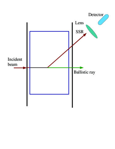
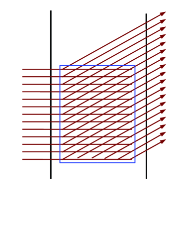
Figure 2: (Color online) (a) Schematic illustration of the broken-ray (or single-scattered ray, denoted here by SSR) trajectory. (b) Source-detector arrangement for SSOT. Reconstruction is performed independently slice-by slice. The blue rectangle represents the area in which a reconstruction can be performed.

By utilizing multiple incident beams and detecting the light exiting the sample at different points, as shown in Fig. 2(b), we will see that it is possible to collect sufficient data to reconstruct the spatial distribution of the attenuation coefficient in a fixed transverse slice of the slab. In addition to varying the source and detector positions, one can also vary the angles of incidence and detection. In principle, this can provide additional information for simultaneous reconstruction of absorption and scattering coefficients of the sample, a topic we will consider elsewhere.

The image reconstruction problem of SSOT is to reconstruct $\mu_{a}$, $\mu_{s}$ and $A$ from measurements of $I_{s}$. For simplicity, we assume that $\mu_{s}$ and $A$ are known, in which case we wish to determine $\mu_{a}$. To proceed, we use Eq. (13) to separate the known or measured quantities from those that need to be reconstructed, and introduce the data function

$$\phi({\bf r}_{1},\hat{\bf s}_{1};{\bf r}_{2},\hat{\bf s}_{2})=-\ln\left[\frac{r_{21}\sin\theta_{1}\sin\theta_{2}\int I_{s}({\bf r}_{1},\hat{\bf s}_{1};{\bf r}_{2},\hat{\bf s}_{2})d\varphi_{\hat{\bf s}_{2}}}{I_{0}\mu_{s}A(\hat{\bf s}_{1},\hat{\bf s}_{2})}\right]\ ,$$ (16)

where we have assumed that $A$ is position-independent. Note that if $I_{s}$ is experimentally measured, the angular integration on the right-hand side of (16) does not need to be performed numerically. The measured data is necessarily integrated in a narrow interval of $\varphi_{\hat{\bf s}_{2}}$ due to the finite aperture and acceptance angle of the detector. Note also that the above definition is only applicable for such configurations of sources and detectors such that $\theta_{1}+\theta_{2}<\pi$. Otherwise, any measured intensity is due to higher-order terms in the collision expansion which are not accounted for (13).

Making use of the definition (16) and Eq. (13), we find that $\mu_{t}$ obeys the integral equation

$$\phi({\bf r}_{1},\hat{\bf s}_{1};{\bf r}_{2},\hat{\bf s}_{2})=\int_{{\rm BR}({\bf r}_{1},\hat{\bf s}_{1};{\bf r}_{2},\hat{\bf s}_{2})}\mu_{t}({\bf r}(\ell))d\ell\ .$$ (17)

Here the integral is evaluated along the broken ray (such as the one shown in Fig. 1), which is uniquely defined by the source and detector positions and orientations, and $\ell$ is the linear coordinate along the ray.

According to (17), the attenuation function is linearly related to the data function. In this respect, the mathematical structure of SSOT is similar to the problem of inverting the Radon transform in computed tomography except that the integrals are evaluated along broken rays. Since $\mu_{t}$ may be regarded as a function of two variables, it is sufficient to consider only two-dimensional measurements. One possible choice is to vary the source and detector coordinates, $y_{1}$ and $y_{2}$, while keeping the angles of incidence and detection $\beta_{1}$ and $\beta_{2}$ fixed. By $\beta_{1}$ and $\beta_{2}$ we mean here the angles between the $z$-axis of the laboratory frame and the unit vectors $\hat{\bf s}_{1}$ and $\hat{\bf s}_{2}$, respectively. Note that these angles are not equal to the angles $\theta_{1}$ and $\theta_{2}$ shown in Fig. 1. The latter can vary in the measurement scheme described in this section, while $\beta_{1}$ and $\beta_{2}$ are fixed. Below, we omit $\beta_{1}$ and $\beta_{2}$ from the list of formal arguments of the data function and consider the equation

$$\phi(y_{1},y_{2})=\int_{{\rm BR}(y_{1},y_{2})}\mu_{t}(y(\ell),z(\ell))d\ell\ ,$$ (18)

where $\phi(y_{1},y_{2})$ is the two-dimensional data function.

As explained above, the selection of the points and directions of incidence and detection define a slice in which $\mu_{t}$ is to be reconstructed. In Fig. 1, this slice coincides with the $yz$-plane of the laboratory frame. Assuming that the $x$-coordinate is fixed, we then regard $\mu_{t}$ as a function of $y$ and $z$. Three-dimensional reconstruction is then performed slice-by-slice.

IV Image Reconstruction

In this section we illustrate image reconstruction in SSOT using a numerical technique based on discretization and algebraic inversion of the two-dimensional integral equation (18). We note that more sophisticated image reconstruction procedures which utilize the translational invariance of rays may also be derived. These methods are conceptually similar to those previously developed for optical diffusion tomography schotland_01_1 ; markel_04_4 and will be described elsewhere.

IV.1 Forward Problem

We begin by describing a method to generate simulated forward data to test the SSOT image reconstruction. Assuming an isotropically scattering sample with $A(\hat{\bf s},\hat{\bf s}^{\prime})=1/4\pi$, it can be shown from (3) erdmann_68_1 ; larsen_74_1 that the specific intensity everywhere inside the sample is related to the density of electromagnetic energy $u({\bf r})\equiv\int I({\bf r},\hat{\bf s})d^{2}{s}$ by the formula

$$I({\bf r},\hat{\bf s})=I_{b}({\bf r},\hat{\bf s})+\frac{1}{4\pi}\int G({\bf r},\hat{\bf s};{\bf r}^{\prime},\hat{\bf s}^{\prime})\mu_{s}({\bf r}^{\prime})u({\bf r}^{\prime})d^{3}r^{\prime}d^{2}{s}^{\prime},$$ (19)

where $u({\bf r})$ satisfies the integral equation

$$u({\bf r})=u_{b}({\bf r})+\frac{1}{4\pi}\int g({\bf r},{\bf r}^{\prime})\mu_{s}({\bf r}^{\prime})u({\bf r}^{\prime})d^{3}r^{\prime}\ ,$$ (20)

Here $g({\bf r},{\bf r}^{\prime})$ is given by (7) and $u_{b}({\bf r})\equiv\int I_{b}({\bf r},\hat{\bf s})d^{2}s$ is the ballistic energy density. We note that the assumption of isotropic scattering is the most stringent test for SSOT.

The specific intensity is computed by first solving the integral equation (20) and then substituting the obtained solution $u({\bf r})$ into (19) (where the ballistic part $I_{b}$ may be ignored). Note that $I({\bf r},\hat{\bf s})$ calculated from (19) satisfies the boundary conditions at all surfaces. We also stress that this numerical approach is non-perturbative and includes all orders of scattering.

In the simulations shown below, (20) is discretized on a rectangular grid and solved by standard methods of linear algebra. The energy density $u({\bf r})$ is assumed constant within each cubic cell, and the corresponding values $u_{n}=u({\bf r}_{n})$, where ${\bf r}_{n}$ is the center of the $n$th cubic cell, obey the algebraic system of equations obtained by discretizing Eq. (20). The off-diagonal elements of the matrix of this system corresponding to the integral on the right-hand side of (20) are given by $(\mu_{s}h^{3}/4\pi)g({\bf r}_{m},{\bf r}_{n})$, where $h$ is the discretization step. Here we can take advantage of the fact that $\mu_{s}$ was set to be constant throughout the sample, while the inhomogeneities were assumed to be purely absorbing. Computation of the diagonal elements is slightly more involved because $g({\bf r},{\bf r}^{\prime})$ diverges when ${\bf r}\rightarrow{\bf r}^{\prime}$. In this case, we need to find an approximation for the integral

$$S=\frac{\mu_{s}}{4\pi}\int_{V_{n}}g({\bf r}_{n},{\bf r})d^{3}r\ ,$$ (21)

where the integration is carried out over the $n$th cell. While integration over a cubic volume is difficult, the important fact is that the singularity in $g({\bf r},{\bf r}^{\prime})$ is integrable. We then write, approximately,

$$S\approx\mu_{s}\int_{0}^{R_{\rm eq}}g(0,{\bf r})r^{2}dr\ ,$$ (22)

where $R_{\rm eq}=(3/4\pi)^{1/3}h$ is the radius of a sphere of equivalent volume. For a sufficiently fine disctretization, $\mu_{t}R_{\rm eq}\ll 1$, which allows us to write $g(0,{\bf r})\approx 1/r^{2}$. This leads to $S=\mu_{s}R_{\rm eq}$, and the discretized version of Eq. (20) becomes

$$(1-\mu_{s}R_{\rm eq})u_{n}-\frac{\mu_{s}h^{3}}{4\pi}\sum_{m\neq n}g({\bf r}_{n},{\bf r}_{m})u_{m}=u_{b}({\bf r}_{n})\ .$$ (23)

We note that this set of equations is an accurate approximation to the integral equation (20) if $\mu_{s}R_{\rm eq}\sim\mu_{s}h\ll 1$. However, since in practice this inequality may be not very strong, the term $\mu_{s}R_{\rm eq}$ on the left-hand side of (23) is not neglected.

Eq. (23) can be written in matrix notation as

$${\mathcal{W}}|u\rangle=|b\rangle$$ (24)

where

$$\langle n|{\mathcal{W}}|m\rangle = \frac{1}{\alpha}\delta_{nm}\$$ (25)

$$-\ \frac{h^{2}}{|{\bf r}_{n}-{\bf r}_{m}|^{2}}\exp\left[-\int_{0}^{|{\bf r}_{n}-{\bf r}_{m}|}\mu_{t}\left({\bf r}_{m}+\hat{\bf u}({\bf r}_{n}-{\bf r}_{m})\ell\right)d\ell\right](1-\delta_{nm})\ ,$$

with $\delta_{nm}$ being the Kronecker delta function, $\alpha$ being a dimensionless coupling constant defined by

$$\alpha=\frac{\mu_{s}h}{4\pi(1-\mu_{s}R_{\rm eq})}\ ,$$ (26)

$\langle n|u\rangle=u_{n}$, and $\langle n|b\rangle=4\pi u_{b}({\bf r}_{n})/\mu_{s}h$. Note that the quantity $u_{b}({\bf r}_{n})$ is defined as an average over the $n$th cell, namely, $u_{b}({\bf r}_{n})=h^{-3}\int_{V_{n}}u_{b}({\bf r})d^{3}r$.

Computing the elements of the matrix ${\mathcal{W}}$ requires the evaluation of the integrals on the right-hand side of (25). For a homogeneous sample, this can be performed analytically. For an inhomogeneous sample, it is done numerically. Once this is accomplished, (24) is then solved by matrix inversion. We note that the symmetric matrix ${\mathcal{W}}$ is well-conditioned condition-number . This is illustrated in Fig. 3 where we plot all the eigenvalues of ${\mathcal{W}}$ for $\mu_{s}=0.08h^{-1}$ with the set of absorbing inhomogeneities described in section IV.3. We also note that ${\mathcal{W}}$ is positive-definite, so that $u$ and $u_{b}$ are positive. Also, it was verified in all simulations that the diffuse component of the density, defined as the quantity $u-u_{b}$, was positive everywhere inside the sample.

Figure 3: (Color online) All $53,680$ eigenvalues $w_{n}$ of the matrix ${\mathcal{W}}$ of Eq. 24 computed for $\mu_{s}=0.08h^{-1}$ and the set of absorbing inhomogeneities described in section IV.2.

Special attention must be given to the effects of discretization when computing the single-scattered intensity, the data function, and the forward data. Since the computations involve discrete rays, employing the expressions (13) and (16) that contain the delta-function $\delta\left(|\varphi_{\hat{\bf s}_{1}}-\varphi_{\hat{\bf s}_{2}}|-\pi\right)$ and the geometrical factor $1/r_{21}\sin\theta_{2}\sin\theta_{1}$ becomes cumbersome. Instead, we have derived the discrete analogues of these expressions starting form Eq. (12) from which (13) has been obtained. In particular, the expression for the single-scattered intensity (the discrete analog of (13)) is obtained from Eq. (12) as

$$I_{s}({\bf r}_{2},\hat{\bf s}_{2};{\bf r}_{1},\hat{\bf s}_{1})=\frac{\mu_{s}h^{3}}{4\pi}g({\bf r}_{2},{\bf R}_{21})u_{b}({\bf R}_{21})\ ,$$ (27)

where $u_{b}({\bf R}_{21})$ is the average of $u_{b}({\bf r})$ over the cell that contains ${\bf R}_{21}$. This expression and the expression (5) for the ballistic intensity suggest the definition of the data function of the form

$$\phi({\bf r}_{2},\hat{\bf s}_{2};{\bf r}_{1},\hat{\bf s}_{1})=-{\mbox{l}n}\left[\frac{4\pi}{h^{3}}\frac{I_{s}({\bf r}_{2},\hat{\bf s}_{2};{\bf r}_{1},\hat{\bf s}_{1})}{I_{0}\mu_{s}}\right].$$ (28)

This is the discrete analogue of (16). Finally, the data function is calculated according with this expression and using the specific intensity obtained from the discretized version of (19),

$$I({\bf r}_{2},\hat{\bf s}_{2};{\bf r}_{1},\hat{\bf s}_{1})=\frac{\mu_{s}h^{3}}{4\pi}\sum_{{\bf r}_{2}-{\bf r}_{n}=\hat{\bf s}_{2}|{\bf r}_{2}-{\bf r}_{n}|}g({\bf r}_{2},{\bf r}_{n})u_{n}\ ,$$ (29)

where $u_{n}$ must be computed numerically for the selected source. The condition on the sum means that summation is performed only over cells that are intersected by the ray exiting from the detection point ${\bf r}_{2}$ in the direction $\hat{\bf s}_{2}$. The above formula is valid for the specific measurement scheme which obtains when the intersection length of all such rays with any cubic cell is constant. Otherwise, a more complicated numerical integration must be employed. We note while Eqs. (28) and (29) are employed for simulated data, Eqs. (13) and (16) must be used when experimental data is available. Also, the use of experimental data avoids many mathematical complications that arise due to discretization of rays, needed to solve the forward RTE problem, usually computationally intensive.

In order to model the noise in measured data, the specific intensity obtained from the forward solver was scaled and rounded so that it was represented by 16-bit unsigned integers, similar to the measurement by a typical CCD camera. Then a statistically-independent positively-defined random variable was added to each measurement. The random variables were evenly distributed in the interval $[0,nI_{\rm av}]$, where $n$ is the noise level indicated in the figure legends below and $I_{\rm av}$ is the average measured intensity (a 16-bit integer). The DC part (the positive background) of the intensity was not subtracted (this procedure is commonly applied to the digital output of CCD chips). Then the simulated intensity measurements, together with the appropriately scaled incident intensity $I_{0}$ were substituted into (16) to obtain the data function $\phi$.

IV.2 Inverse Problem

We now describe the method by which we invert the integral equation (18). The discrete version of (18) has the form

$$\sum_{n}{\mathcal{L}}_{\nu n}\mu_{tn}=\phi_{\nu}\ ,$$ (30)

where the same grid is employed as is used to solve the forward problem, ${\mathcal{L}}_{\nu n}$ is the length of the intersection of the broken ray indexed by $\nu=(y_{1},y_{2})$ with the $n$th cubic cell (located within the selected $x$-slice of the sample). The matrix elements ${\mathcal{L}}$ are determined from simple geometric considerations. The matrix form of (30) is

$${\mathcal{L}}|\mu_{t}\rangle=|\phi\rangle\ .$$ (31)

The equation (31) can be solved using a regularized pseudoinverse natterer_book_01 , namely,

$$|\mu_{t}^{+}\rangle=({\mathcal{L}}^{*}{\mathcal{L}})^{-1}{\mathcal{L}}^{*}|\phi\rangle\ .$$ (32)

Here $({\mathcal{L}}^{*}{\mathcal{L}})^{-1}$ is understood in the following sense:

$$({\mathcal{L}}^{*}{\mathcal{L}})^{-1}=\sum_{n}\Theta(\sigma_{n}^{2}-\epsilon)\frac{|f_{n}\rangle\langle f_{n}|}{\sigma_{n}^{2}}\ ,$$ (33)

where $\Theta(x)$ is the step function, $\epsilon$ is a small regularization parameter, and $|f_{n}\rangle$ and $\sigma_{n}$ are the singular vectors and singular values  natterer_book_01 , respectively, of the matrix ${\mathcal{L}}$. These quantities are the solution of the symmetric eigenproblem ${\mathcal{L}}^{*}{\mathcal{L}}|f_{n}\rangle=\sigma_{n}^{2}|f_{n}\rangle$. A typical spectrum of singular values of ${\mathcal{L}}$ for $\mu_{s}=0.08h^{-1}$, $1,600$ measurements and $34^{2}=1,156$ unknown values of $\mu_{t}$ (the size of ${\mathcal{L}}$ in this example is $1,600\times 1,156$, so that the problem is slightly overdetermined) is shown in Fig. 4. It can be seen that matrix condition number condition-number for the inverse problem is much larger than for the forward problem. In the example shown in Fig. 4, the condition number is $\approx 10^{3}$. Thus the inverse problem is very mildly ill-posed.

Figure 4: (Color online) All $1,156$ non-zero singular values $\sigma_{n}$ of the matrix ${\mathcal{L}}$ defined by Eq. (30) (the size of ${\mathcal{L}}$ in this example is $1,600\times 1,156$).

IV.3 Numerical Results

In what follows, we illustrate applications of SSOT to biological imaging. In particular, the numerical simulations presented here are relevant for “semi-transparent” systems, such as zebra fish or engineered tissues. Also, the physical situations analyzed here are experimentally encountered for organ tissues at certain wavelengths of the illuminating beam welch_book .

Reconstructions were carried out for a rectangular isotropically scattering sample of dimensions $L_{x}=25h$, $L_{y}=122h$ and $L_{z}=40h$. The background absorption coefficient of the sample was equal to $0.01h^{-1}$ and was spatially modulated by absorbing inhomogeneities (the target). The target was a set of absorbing inclusions formed in the shape of letters, with absorption varying from $0.06h^{-1}$ to $0.2h^{-1}$. The inclusions were concentrated only in three layers: $x=6h$, $x=13h$ and $x=20h$, as shown in the columns marked model of Figs. 5-7. The scattering coefficient was constant throughout the sample, with three different values used throughout the simulations corresponding to $\mu_{s}=0.04h^{-1}$, $\mu_{s}=0.08h^{-1}$ and $\mu_{s}=0.16h^{-1}$. Thus, for example, in the case $\mu_{s}=0.04h^{-1}$ the contrast of $\mu_{t}$ (the ratio of $\mu_{t}$ in the target to the background value) varied from $2.0$ in the letters RADIOL to $4.8$ in the letters DEPT. In the case $\mu_{s}=0.16h^{-1}$, the contrast was smaller and varied from $1.18$ to $2.12$. We note that the contrast in the total attenuation coefficient depends weakly on the background absorption coefficient, compared to its dependence on the background scattering coefficient.

The sources were normally incident on the surface $z=0$. The detectors were placed on the opposite side of the sample and the specific intensity exiting the surface $z=L_{z}$ at the angle of $\pi/4$ with respect to the $z$-axis was measured. In this situation there are two possibilities—the exiting rays either make an angle of $\pi/4$ or $3\pi/4$ with the $y$-axis. In some cases, data from both directions were used. Note that the distance $L_{z}$ corresponds to the slab thickness $L$ used in Sec. II. The optical depth of the sample, $\mu_{s}L_{z}$, varied from $1.6$, for $\mu_{s}=0.04h^{-1}$, to $6.4$, for $\mu_{s}=0.16h^{-1}$ . This corresponds to the mesoscopic scattering regime in which the image reconstruction method of SSOT is applicable.

Reconstruction of the total attenuation coefficient $\mu_{t}$ was performed in slices $x=x_{\rm slice}$ separated by a distance $\Delta x=h$. For each slice, the source positions were $x=x_{\rm slice}$, $y=nh$, $z=0$, with $n$ being integers. The reconstruction area inside each slice was $44h\leq y\leq 77h$, $4h\leq z\leq 37h$, with the field of view $34h\times 34h$. At the noise levels $n=0$ and $n=1\%$, only the rays making an angle of $\pi/4$ with the $y$-axis were used; for the noise level $n=3\%$, the exiting rays which make an angle of $3\pi/4$ with the $y$-axis were also used in order to improve image quality of the reconstructions. Also, the regularization parameter $\epsilon$ in the regularized pseudoinverse (33) was varied to obtain the best visual appearance of images. Note that the absolute values of the reconstructed $\mu_{t}$ are not sensitive to the choice of $\epsilon$. Qualitatively, the same results are obtained by setting $\epsilon=0$, although we have found that selecting a small but nonzero value of $\epsilon$ tends to slightly improve image quality.

The results of image reconstructions for various noise levels are presented in Figs. 5–7, where we show both slices containing inhomogeneities and neighboring slices in which inhomogeneities are not present. It can be seen that the spatial resolution depends on the noise level and contrast, and can be as good as one discretization step, $h$. Note that the reconstructed images are in very good quantitative agreement with the model (all panels in each figure are plotted using the same color scale) and stable in the presence of noise. When $\mu_{s}=0.16h^{-1}$ (Fig. 7) the optical depth of the sample is $\mu_{s}L_{z}=6.4$. This is a borderline case when scattering is sufficiently strong so that the single-scattering approximation of SSOT may be expected to be inaccurate. Indeed, the image quality in Fig. 7 is markedly worse than in Figs. 5 and 6, yet the letters in the image remain legible.

We emphasize that the reconstructed images presented here are based on simulated data obtained by solving the RTE exactly, thereby accounting for all orders of scattering. For samples which are optically thick, the resulting reconstructions evidently exhibit artifacts due to the breakdown of the single scattering approximation (which is not possible physically but achievable in simulations). Such would be absent if only single-scattered light were detected. To illustrate this idea, we present in Fig. 8 reconstructed images for the case $\mu_{s}=0.16h^{-1}$ using forward data in which only single-scattered light is retained. Here, instead of solving the full RTE, the data function was directly calculated from (17). The aforementioned procedure of generating data overestimates the performances of the imaging method. It can be seen from Fig. 8 that, as expected, significantly better reconstructions result.

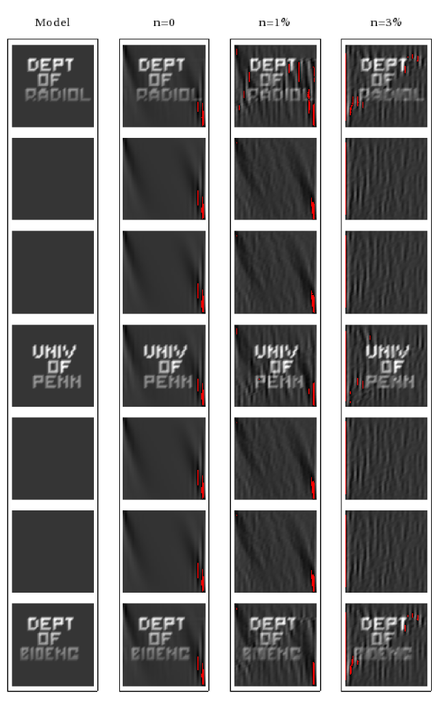
Figure 5: (Color online) Image reconstruction for a slab with $\mu_{s}=0.04h^{-1}$ and various noise levels $n$. The absorbing inhomogeneities are placed in the slices $x=6h$, $x=13h$ and $x=20h$, and the rows show the slices $x=6h$, $7h$, $12h$, $13h$, $14h$, $19h$, and $20h$. The same color scale is used for all slices, with the maximum (white) corresponding to $\mu_{t}=0.24h^{-1}$ and the minimum (black) to $\mu_{t}=0$. Red regions correspond to negative values of the reconstructed extinction coefficient.

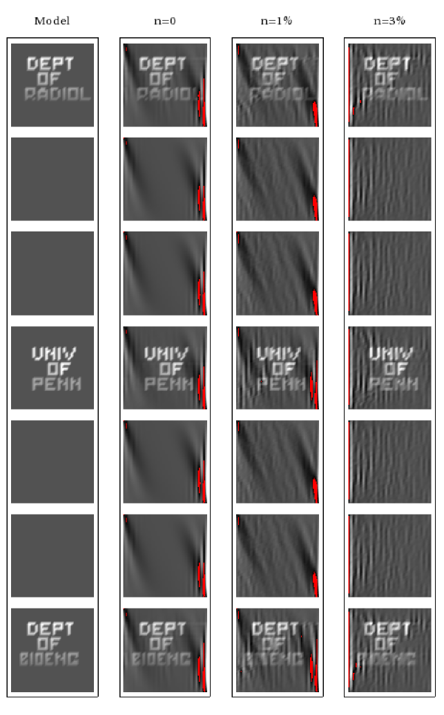
Figure 6: (Color online) Image reconstruction for a slab with $\mu_{s}=0.08h^{-1}$. The same color scale is used for all slices, with the maximum (white) corresponding to $\mu_{t}=0.28h^{-1}$ and the minimum (black) to $\mu_{t}=0$. All the other details are as for Fig. 5.

Figure 7: (Color online) Image reconstruction for a slab with $\mu_{s}=0.16h^{-1}$. The same color scale is used for all slices, with the maximum (white) corresponding to $\mu_{t}=0.36h^{-1}$ and the minimum (black) to $\mu_{t}=0$. All the other details are as for Fig. 5.

Figure 8: (Color online) Image reconstruction for $\mu_{s}=0.16h^{-1}$, for a data function corresponding only to single-scattered light and calculated according to (18). All the other details are as for Fig. 7.

V Discussion

We have investigated the problem of optical tomography in the mesoscopic regime. Within the accuracy of the single scattering approximation to the RTE, we have derived a relation between the absorption and scattering coefficients and the specific intensity. In particular, for a homogeneously scattering medium, we have shown that the intensity measured by an angularly-selective detector is related to the integral of the attenuation coefficient along a broken ray. By inverting this relation, we are able to recover the attenuation coefficient of the medium.

The image reconstruction technique we have implemented breaks down in the multiple scattering regime. In future work, we plan to explore corrections to the single scattering approximation. In addition, since electromagnetic waves in random media are, in general, polarized, we also intend to explore the effects of polarization within the framework of the generalized vector radiative transport equation ishimaru . Finally, we note that a technique for fluorescence imaging of mesoscopic objects has recently been reported ntziachristos . It would thus be of interest to investigate the fluorescent analog of SSOT.

Appendix A Derivation of Eq. (13)

Substitution of (5) into (12) with ${\bf r}={\bf r}_{2}$ and $\hat{\bf s}=\hat{\bf s}_{2}$ results in the following expression for the single-scattered intensity:

$$I_{s}({\bf r}_{1},\hat{\bf s}_{1};{\bf r}_{2},\hat{\bf s}_{2})=I_{0}A(\hat{\bf s}_{2},\hat{\bf s}_{1})\int\mu_{s}({\bf r})g({\bf r}_{2},{\bf r})g({\bf r},{\bf r}_{1})$$

$$\hskip 28.45274pt\times\delta(\hat{\bf u}({\bf r}_{2}-{\bf r})-\hat{\bf s}_{2})\delta(\hat{\bf u}({\bf r}-{\bf r}_{1})-\hat{\bf s}_{1})d^{3}r\ ,$$ (34)

where we have introduced the notation $\hat{\bf u}({\bf r})={\bf r}/r$. In the following analysis, the manipulation of delta functions is done in accordance with the theory of generalized functions Lighthill_book .

We now make the change of variables ${\bf r}={\bf r}_{1}+{\bf R}$, ${\bf R}=R\hat{\bf R}$ and $d^{3}r=d^{3}R=R^{2}dRd^{2}\hat{R}$. The integral over $d^{2}\hat{R}$ is immediately evaluated and (34) becomes

$$I_{s}({\bf r}_{1},\hat{\bf s}_{1};{\bf r}_{2},\hat{\bf s}_{2})=I_{0}A(\hat{\bf s}_{2},\hat{\bf s}_{1})\int g({\bf r}_{2},{\bf r}_{1}+R\hat{\bf s}_{1})g({\bf r}_{1}+R\hat{\bf s}_{1},{\bf r}_{1})$$

$$\hskip 28.45274pt\times\mu_{s}({\bf r}_{1}+R\hat{\bf s}_{1})\delta(\hat{\bf u}({\bf r}_{21}-R\hat{\bf s}_{1})-\hat{\bf s}_{2})R^{2}dR\ .$$ (35)

We then write the remaining delta-function as

$$\delta(\hat{\bf u}-\hat{\bf s}_{2})=\delta(\varphi_{\hat{\bf u}}-\varphi_{\hat{\bf s}_{2}})\delta\left(\cos\theta_{\hat{\bf u}}-\cos\theta_{\hat{\bf s}_{2}}\right)\ .$$ (36)

Here ${\bf u}={\bf r}_{21}-R\hat{\bf s}_{1}$ and $\theta$ and $\varphi$ are polar angles of the respective unit vectors. It is convenient to work in a reference frame whose $z$-axis coincides with the source-detector line. We then find that $\varphi_{\hat{\bf u}}=\varphi_{\hat{\bf s}_{1}}\pm\pi$. Consequently,

$$\delta(\varphi_{\hat{\bf u}}-\varphi_{\hat{\bf s}_{2}})=\delta\left(|\varphi_{\hat{\bf s}_{1}}-\varphi_{\hat{\bf s}_{2}}|-\pi\right)\ .$$ (37)

We next write

$$\delta\left(\cos\theta_{\hat{\bf u}}-\cos\theta_{\hat{\bf s}_{2}}\right)=\delta(f(R))\ ,$$ (38)

where

$$f(R)=\frac{r_{21}-R\cos\theta_{1}}{\sqrt{r_{21}^{2}-2r_{21}R\cos\theta_{1}+R^{2}}}-\cos\theta_{2}\ .$$ (39)

It can be verified that if $\theta_{1}+\theta_{2}\geq\pi$, the equation $f(R)=0$ has no positive roots. In the opposite limit, however, there is one positive root $R=L_{1}$. Note that the lengths $L_{1}$ and $L_{2}$ are defined by (15) and illustrated in Fig. 1. We thus have

$$R^{2}\delta(f(R))=\Theta(\pi-\theta_{1}-\theta_{2})L_{1}^{2}\frac{\delta(R-L_{1})}{|f^{\prime}(L_{1})|}\ .$$ (40)

Computation of the above derivative is straightforward and yields

$$|f^{\prime}(L_{1})|=\frac{L_{1}}{r_{21}L_{2}\sin^{2}(\theta_{1}+\theta_{2})}\ .$$ (41)

Collecting everything, we arrive at

$$R^{2}\delta(\hat{\bf u}({\bf r}_{21} - R\hat{\bf s}_{1})-\hat{\bf s}_{2})=$$ (42)

$$\delta\left(|\varphi_{\hat{\bf s}_{1}}-\varphi_{\hat{\bf s}_{2}}|-\pi\right)\Theta(\pi-\theta_{1}-\theta_{2})\frac{r_{21}L_{1}L_{2}\delta(R-L_{1})}{\sin^{2}(\theta_{1}+\theta_{2})}\ .$$

We then recall that ${\bf r}_{1}+L_{1}\hat{\bf s}={\bf R}_{21}$, $L_{1}=|{\bf R}_{21}-{\bf r}_{1}|$, $L_{2}=|{\bf r}_{2}-{\bf R}_{21}|$ and obtain

$$g({\bf r}_{2},{\bf r}_{1}+L_{1}\hat{\bf s}_{1}) = \frac{1}{L_{2}^{2}}\exp\left[-\int_{0}^{L_{2}}\mu_{t}({\bf R}_{21}+\hat{\bf s}_{2}\ell)d\ell\right]\ ,$$ (43)

$$g({\bf r}_{1}+L_{1}\hat{\bf s}_{1},{\bf r}_{1}) = \frac{1}{L_{1}^{2}}\exp\left[-\int_{0}^{L_{1}}\mu_{t}({\bf r}_{1}+\hat{\bf s}_{1}\ell)d\ell\right]\ .$$ (44)

Finally, using (15), we arrive at the result (13).

References

- (1) T. Wilson and C.J.R. Sheppard, Theory and Practice of Scanning Optical Microscopy (Academic Press, 1984).
- (2) J.A. Izatt, M.R. Hee, G.M. Owen, E.A. Swanson, and J.G. Fujimoto, Opt. Lett. 19, 590 (1994).
- (3) J. Sharpe, U. Ahlgren, P. Perry, B. Hill, A. Ross, J. Hecksher-Sorensen, R. Baldock and D. Davidson, Science 296, 541 (2002).
- (4) T.S. Ralston, D.L. Marks, P.S. Carney and S.A. Boppart, J. Opt. Soc. Am. A 23, 1027(2006).
- (5) T.S. Ralston, D.L. Marks, P.S. Carney and S.A. Boppart, Nature Physics 3, 129 (2007).
- (6) S. Arridge, Inv. Prob. 15, R41 (1999).
- (7) M.C.W. van Rossum and Th.M. Nieuwenhuizen, Rev. Mod. Phys. 71, 313 (1999).
- (8) A. Ishimaru, Wave Propagation and Scattering in random Media (IEEE, 1997).
- (9) J. J. Duderstadt, W. R. Martin, Transport theory (John Wiley and Sons, 1979).
- (10) J. C. Schotland and V. A. Markel, J. Opt. Soc. Am. A, vol. 18, no. 11, pp. 2767–2777, 2001.
- (11) V. A. Markel and J. C. Schotland, Phys. Rev. E, vol. 70, no. 5, p. 056616(19), 2004.
- (12) R. C. Erdmann and C. E. Siewert, J. Math. Phys., vol. 9, no. 1, pp. 81–89, 1968.
- (13) E. W. Larsen, J. Math. Phys., vol. 15, no. 3, pp. 299–305, 1974.
- (14) The measure of how numerically well-conditioned the problem associated with solving the linear equation is the condition number of the matrix . This can be regarded as the rate at which the solution, , changes with respect to a change in , and can be calculated as the ratio between the maximal and minimal singular values of , respectively. A problem with a low condition number is said to be well-conditioned, while a problem with a high condition number is said to be ill-conditioned.
- (15) F. Natterer and F. Wubbeling, Mathematical methods in image reconstruction. Philadelphia: SIAM, 2001.
- (16) A. J. Welch and M. J. C. van Gemert, Optica-thermal response of laser-irradiated tissue (Plenum Press, 1995).
- (17) C. Vinegoni, C. Pitsouli, D. Razansky, N. Perrimon, V. Ntziachristos, Nature Methods 5, 45 (2008).
- (18) M. J. Lighthill, Fourier Analysis and Generalized Functions (Cambridge U. P., Cambridge, England, 1960)