Subwavelength resolution with three-dimensional isotropic transmission-line lenses

Abstract

Dispersion, impedance matching and resolution characteristics of an isotropic three-dimensional flat lens (“superlens”) are studied. The lens is based on cubic meshes of interconnected transmission lines and bulk loads. We study a practical realization of the lens, based on the microstrip technology. The dispersion equations that have been previously derived, are verified with full-wave simulations. The isotropy of the structure is verified with analytical as well as simulation results. The resolution characteristics of a practically realizable, lossy lens are studied analytically.

I Introduction

Materials with simultaneously negative material parameters (double-negative or backward-wave materials, where permittivity $\varepsilon$ and permeability $\mu$ are both effectively negative) [1] have received a lot of interest in the recent literature. One of the most exciting applications of these materials is a device capable of subwavelength resolution (resolution that exceeds the diffraction limit) [2]. The first demonstrations of realized artificial backward-wave materials were done in the microwave region using periodic structures consisting of metal wires (negative $\varepsilon$) and split-ring resonators (negative $\mu$) [3].

Also the use of loaded transmission-line networks has been proposed for the realization of wide-band and low-loss backward-wave materials in the microwave region [4, 5]. These networks are inherently one-or two-dimensional structures [6, 7]. Recently, also three-dimensional, isotropic transmission-line-based backward-wave materials have been proposed [8, 9, 10] and realized [11].

It has been shown that subwavelength imaging of the near-field is possible even without backward-wave materials (note that in these cases the focusing of the propagating modes is not possible). This phenomenon can be achieved with a bulk material slab having negative permittivity or permeability [12], or without any bulk material by using planar sheets supporting surface plasmons [13, 14, 15]. Also devices which operate in the “canalization” regime have been used successfully to obtain subwavelength resolution [16, 17]. Some of the previous methods have also been suggested for use in the optical region [12, 18, 19].

In this paper, we make a detailed study of a three-dimensional, isotropic superlens based on loaded transmission-line networks. This approach to superlens design that we use here was originally proposed in [10]. Here we confirm the isotropy of the structure by studying the dependence of the dispersion on the direction of propagation and verify the analytical design equations presented in [10] with full-wave simulations. We also confirm that the impedance matching, which is essential for operation of the device, is preserved for all directions of propagation. The resolution enhancement capability of a practically realizable, lossy lens is analytically studied using a method presented in [20]. Although the lens inherently achieves ideal operation at a single frequency only (the dispersion curves of forward-wave and backward-wave materials intersect at a single frequency point), we show that the enhancement of the evanescent modes (which enables subwavelength resolution) is possible in a small frequency band near the optimal operation frequency.

Figure 1: Structure of the superlens. If the source plane is at $z=0$, the image plane is situated at $z=2l$.

II The structure of the lens

We study the superlens structure presented in [10, 11]. The superlens is a combination of two types of transmission-line networks: a region with effectively negative $\varepsilon$ and $\mu$ is sandwiched between two regions possessing effectively positive $\varepsilon$ and $\mu$ (forward-wave regions), see Fig. 1. As was previously shown in [10], the transmission-line networks are easy to realize using the microstrip technology and we continue to use this approach in this paper (the design equations can be applied to other types of transmission lines as well, see [10]). The forward-wave network has a unit cell as shown in Fig. 2. The unit cell of the backward-wave network is otherwise similar to the one shown in Fig. 2, but it is loaded with lumped capacitors of value $2C$ (in series with the microstrip lines) in all of the six branches of the unit cell and an inductor of value $L$ is connected from the center node of the microstrip line to the ground. See [11] for a representation of the unit cell structure of both networks.

Figure 2: The unit cell of a three-dimensional, forward-wave transmission-line network based on the microstrip technology (the substrate is not shown for clarity). The backward-wave unit cell is similar, but with lumped capacitors in each of the six branches of the transmission lines (connected in series) and with a lumped inductor, connected between the center node and the ground.

III Dispersion

The dispersion equations for the forward-wave and backward-wave networks have been derived in [10] and they read (in the lossless case):

$$\cos(q_{x})+\cos(q_{y})+\cos(q_{z})=\frac{1}{2j\omega LS_{\rm BW}}-3\frac{K_{\rm BW}}{S_{\rm BW}}$$ (1)

and

$$\cos(q_{x})+\cos(q_{y})+\cos(q_{z})=-3\frac{K_{\rm FW}}{S_{\rm FW}},$$ (2)

where

$$S_{\rm BW}=\frac{j\omega C}{(D_{\rm t}+j\omega CB_{\rm t})(A_{\rm t}+j\omega CB_{\rm t})+\omega^{2}C^{2}B_{\rm t}^{2}},$$ (3)

$$K_{\rm BW}=\frac{-(B_{\rm t}C_{\rm t}-D_{\rm t}A_{\rm t})(A_{\rm t}+j\omega CB_{\rm t})}{[(D_{\rm t}+j\omega CB_{\rm t})(A_{\rm t}+j\omega CB_{\rm t})+\omega^{2}C^{2}B_{\rm t}^{2}]B_{\rm t}}-\frac{A_{\rm t}}{B_{\rm t}},$$ (4)

$$S_{\rm FW}=\frac{1}{B_{\rm t}(A_{\rm t}+D_{\rm t})},$$ (5)

$$K_{\rm FW}=-\frac{B_{\rm t}C_{\rm t}-D_{\rm t}A_{\rm t}}{A_{\rm t}+D_{\rm t}}\frac{1}{B_{\rm t}}-\frac{A_{\rm t}}{B_{\rm t}},$$ (6)

$$\left[\begin{array}[]{ccc}A_{\rm t}&B_{\rm t}\\ C_{\rm t}&D_{\rm t}\end{array}\right]=\left[\begin{array}[]{ccc}\cos(k_{\rm TL}d/2)&jZ_{0,\rm TL}\sin(k_{\rm TL}d/2)\\ jZ_{0,\rm TL}^{-1}\sin(k_{\rm TL}d/2)&\cos(k_{\rm TL}d/2)\end{array}\right].$$ (7)

In (1)-(6) the indices FW and BW correspond to the dispersion equations of forward- and backward-wave networks, respectively, and $q_{i}=k_{i}d$ (wavenumber normalized by the period $d$), where $k_{i}$ is the wavenumber in the network along axis $i$. In (7) $k_{\rm TL}$ and $Z_{0,\rm TL}$ are the wavenumber and impedance of the waves in the transmission lines, respectively. Note that $Z_{0,\rm TL}$ is usually different for the forward-wave and backward-wave networks in order to obtain impedance matching of the networks [10].

The parameters of the structure that is studied here are the same as in [11], see Table I ($\varepsilon_{\rm r}$ is the permittivity of the substrate of the microstrip lines). Dispersion curves of the forward-wave and backward-wave networks can be studied analytically using (1)-(7). The unit cells of the both networks have also been simulated with Ansoft HFSS full-wave simulator to obtain the dispersion curves for both networks. See Fig. 3 for the dispersion curves when a planewave is considered ($k_{x}=k_{y}=0$). The simulation results agree very well for all axial directions (practically identical plots). From Fig. 3 we can conclude that the optimal operation frequency of the superlens is $f=0.8513$ GHz (the frequency at which the dispersion curves intersect) and at that point the wavenumber has value $k_{z}\approx 47.65$ 1/m.

TABLE I: Parameters of the superlens structure.

$d$	$Z_{\rm 0,TL,FW}$	$Z_{\rm 0,TL,BW}$	$C$	$L$	$\varepsilon_{\rm r}$
13 mm	$66$ $\Omega$	$89$ $\Omega$	3.3 pF	6.8 nH	2.33

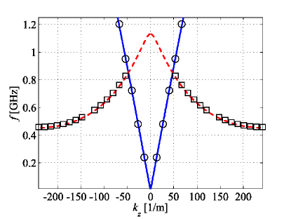
Figure 3: Dispersion curves for the forward-wave (solid line: analytical; circles: HFSS) and backward-wave (dashed line: analytical; squares: HFSS) networks. Propagation along the $z$-axis is considered ($k_{x}=k_{y}=0$).

From (1) and (2) we clearly see that if we consider diagonal propagation ($k_{x}$, $k_{y}$ and $k_{z}$ may all be nonzero depending on the direction of propagation), this introduces some anisotropy to the dispersion. To study this effect, we have analyzed propagation in the structure in other than the axial directions. It has been seen that for the backward-wave network the isotropy is achieved in a large bandwidth below and above the second stopband (for this example, the isotropic region is approximately from 0.5 GHz to 2 GHz), and for the forward-wave network at low frequencies (for this example, below 2 GHz). The operation frequency of the designed lens is well within this isotropic region for both networks. The optimal operation frequency obtained here differs slightly from the one previously presented for a similar structure [11]. The reason for this is that here we have assumed the effective permittivity of the transmission lines to be equal to $\varepsilon_{\rm r}$ (to simplify comparison between the analytical and simulation results).

See Figs. 4 and 5 for the results considering different propagation directions. Note that for the diagonal propagation, the dispersion curves extend to larger values of $k_{\rm tot}=\sqrt{k_{x}^{2}+k_{y}^{2}+k_{z}^{2}}$ than it is shown in Figs. 4 and 5 (these regions are not of interest for superlens operation). The HFSS simulation results agree very well for all of the presented curves. For clarity only the diagonal propagation corresponding to the case with $k_{x}=k_{y}=k_{z}$ is presented (squares and circles).

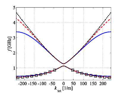
Figure 4: Dispersion curves for the backward-wave network. Solid line: $k_{x}=k_{y}=0$; dashed line: $k_{y}=0$, $k_{x}=k_{z}$; dotted line: $k_{x}=k_{y}=k_{z}$; squares: $k_{x}=k_{y}=k_{z}$ (HFSS).

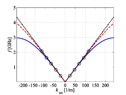
Figure 5: Dispersion curves for the forward-wave network. Solid line: $k_{x}=k_{y}=0$; dashed line: $k_{y}=0$, $k_{x}=k_{z}$; dotted line: $k_{x}=k_{y}=k_{z}$; circles: $k_{x}=k_{y}=k_{z}$ (HFSS).

IV Impedance matching

As was shown in [10, 11], the impedance matching is crucial for the operation of the superlens. Here we use the equations derived for the characteristic impedances of the forward-wave and backward-wave networks [10] to see if the matching is preserved for all propagation directions. In the following we study the matching analytically and tune the impedances of the transmission lines slightly to obtain optimal resolution performance (in [11] and in the previous section the impedance values were not ideal due to the fact that the values were taken from an experimental prototype). It was found that by changing the impedance of the forward-wave transmission lines to $Z_{0,\rm TL,FW}=69.46$ $\Omega$, the wavenumbers and the characteristic impedances of the networks can be matched at the frequency $f=0.8513$ GHz. In the rest of this paper, we use this impedance value and the other design characteristics stay the same as shown in Table I.

See Fig. 6 for the characteristic impedances of the both networks for different propagation directions. Note that because we are interested in the matching between the two networks, the characteristic impedance is defined as the ratio of the voltage and the $z$-component of the current (as was done in [10, 11]). We see that although the values of the impedances change as the direction of propagation changes (naturally, because the impedance depends on $k_{z}$), the matching is preserved for different propagation directions at the operation frequency ($f=0.8513$ GHz).

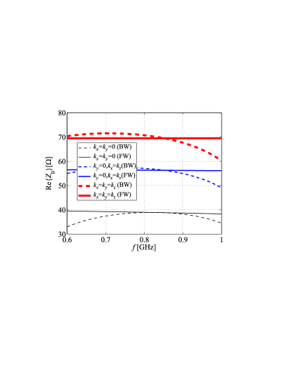
Figure 6: The characteristic impedances of forward-wave and backward-wave networks for different propagation directions.

V Resolution characteristics

V-A Resolution enhancement

To evaluate the performance of the designed lens, we adopt the same method of calculating the resolution enhancement as in [20], where the resolution enhancement was defined for a two-dimensional (planar) lens as:

$$R_{e}=\frac{k_{t\rm,max}}{k_{0}},$$ (8)

where $k_{t\rm,max}$ is the maximum transverse wavenumber that is transmitted from the source plane to the image plane and $k_{0}$ is the maximum transverse wavenumber corresponding to propagating modes ($k_{0}\approx 47.65$ 1/m for the lens that we study here, as can be seen from Fig. 3). Because we consider a three-dimensional lens, the transverse wavenumber is now defined as $k_{t}=\sqrt{k_{x}^{2}+k_{y}^{2}}$, see Fig. 1.

In [20], $k_{t\rm,max}$ was derived analytically from the dimensions of the used superlens (taking into account the effect of losses) as well as calculated from the optical transfer function that was derived analytically and also measured. It was concluded that a good approximation for $k_{t\rm,max}$ is the value of $k_{t}$, at which the absolute value of the optical transfer function drops to 0.5 [20]. In the following, we calculate the transmission coefficient of the lens studied in this paper using the previously derived equations [10]. From the absolute value of the transmission coefficient (which corresponds to the optical transfer function used in [20]) we obtain $R_{e}$ by finding $k_{t\rm,max}$ from the plotted curves as described above.

First, let us see how the thickness of the superlens affects the resolution enhancement. We have calculated the resolution enhancement for the superlens described in the previous sections, taking into account realistic losses caused by the substrate and by the lumped elements (loss tangent of the substrate is $\tan\delta=0.0012$ and the quality factors of the capacitors and inductors are 500 and 50, respectively) [11]. In the calculations, the losses can be taken into account by using complex values for $C$ and $L$ and by replacing (7) by

$$\left[\begin{array}[]{ccc}A_{\rm t}&B_{\rm t}\\ C_{\rm t}&D_{\rm t}\end{array}\right]=\left[\begin{array}[]{ccc}\cosh(\gamma d/2)&jZ_{0,\rm TL}\sinh(\gamma d/2)\\ jZ_{0,\rm TL}^{-1}\sinh(\gamma d/2)&\cosh(\gamma d/2)\end{array}\right],$$ (9)

where

$$\gamma=\frac{\pi\varepsilon_{\rm r}(\varepsilon_{\rm r}-1)\tan\delta}{\sqrt{\varepsilon_{\rm r}}(\varepsilon_{\rm r}-1)\lambda_{0}}+jk_{\rm TL}.$$ (10)

See Fig. 7 for the resolution enhancement as a function of the thickness of the lens (here the thickness refers to the distance from the source plane to the image plane, i.e., thickness is equal to $2l$). Note that when we find $k_{t\rm,max}$ for different thicknesses, the “worst case” is always used. Because of the fact that the impedance values are different for different directions of propagation (see Fig. 6), $k_{t\rm,max}$ is slightly different for various propagation directions. As expected by the results of Fig. 6, $|k_{t\rm,max}|$ is the smallest for the case when $k_{x}=k_{y}$. In the calculation of Fig. 7 and in section V B this “worst case” is used to calculate $R_{e}$.

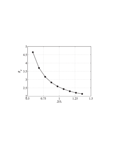
Figure 7: Resolution enhancement of the lens, as a function of the thickness of the lens (distance between source and image) in wavelengths at the optimal operation frequency ($f=0.8513$ GHz). The larger dots show the points in which $R_{e}$ was analytically calculated. Losses of the substrate and the lumped components are taken into account.

V-B Bandwidth

Ideal operation of the superlens described in this paper can be achieved only at a single frequency, as can be seen from Fig. 3. Nevertheless, it is clear that although a small change in the frequency distorts the image seen in the image plane, focusing of the propagating modes and enhancement of the evanescent modes are still expected to happen in some small but finite frequency band. Here we rely on the assumption that the resolution enhancement can still be defined with (8), i.e., the distortion of the image is not very dramatic and $k_{t\rm,max}$ can still be defined as described above. In the following, the operation band is defined as the frequency band where $R_{e}>2$.

First, let us study a lens with the thickness of the backward-wave network being 4 unit cells and the distance between the source and image planes being 8 unit cells. In wavelengths this is $0.78\lambda$ at the center frequency ($f=0.8513$ GHz), because $\lambda=2\pi/k_{0}\approx 0.132$ m. See Fig. 8 for a plot of the transmission coefficient (the absolute value). From Fig. 8 we see that the bandwidth is approximately 2 percent.

Next, we make the lens thinner to see how this affects the bandwidth. Now the thickness of the backward-wave network is 3 unit cells and the distance between the source and image planes is 6 unit cells. In wavelengths this is $0.58\lambda$ at the center frequency. See Fig. 9 for the absolute value of the transmission coefficient corresponding to this case. From Fig. 9 we can conclude that the bandwidth is approximately 6 percent.

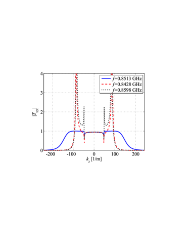
Figure 8: Transmission from the source plane to the image plane as a function of the transverse wavenumber. Solid line: $f=0.8513$ GHz; dashed line: $f=0.8482$ GHz; dotted line: $f=0.8598$ GHz. The band where $R_{e}>2$ is approximately 2 $\%$. The distance between the source and image planes equals $0.78\lambda$ at the center frequency.

VI Conclusions

We have shown that a three-dimensional isotropic transmission-line network can be designed in such a way that the effective permittivity and permeability of the network are negative (a backward-wave material). When combined with a transmission-line network with positive effective permittivity and permeability, the resulting device (superlens) can achieve subwavelength resolution in a small frequency band. In this paper we have verified the previously derived dispersion equations by full-wave simulations and have shown that the designed structure is isotropic in all propagation directions (not just along the three orthogonal ones). We have also confirmed that impedance matching of the two types of networks is possible for an arbitrary direction of propagation. We have analytically studied the effect of losses and the physical size on the resolution and bandwidth characteristics of the designed lens. When high-quality, low-loss components and materials are used, the designed lens can achieve substantial resolution enhancement in a relative bandwidth of a few percents, with the thickness of the lens being of the order of one wavelength.

Figure 9: Transmission from the source plane to the image plane as a function of the transverse wavenumber. Solid line: $f=0.8513$ GHz; dashed line: $f=0.8232$ GHz; dotted line: $f=0.8743$ GHz. The band where $R_{e}>2$ is approximately 6 $\%$. The distance between the source and image planes equals $0.58\lambda$ at the center frequency.

References

- [1] V. G. Veselago, “The electrodynamics of substances with simultaneously negative values of and ,” Sov. Phys. Usp., vol. 10, pp. 509–514, Jan.-Feb. 1968.
- [2] J. B. Pendry, “Negative refraction makes a perfect lens,” Phys. Rev. Lett., vol. 85, pp. 3966–3969, Oct. 2000.
- [3] R. A. Shelby, D. R. Smith, and S. Schultz, “Experimental verification of a negative index of refraction,” Science, vol. 292, pp. 77–79, Apr. 2001.
- [4] C. Caloz, H. Okabe, T. Iwai, and T. Itoh, “Transmission line approach of left-handed (LH) materials,” in Proc. USNC/URSI National Radio Science Meeting, vol. 1, San Antonio, TX, June 2002, p. 39.
- [5] G. V. Eleftheriades, A. K. Iyer, and P. C. Kremer, “Planar negative refractive index media using periodically - loaded transmission lines,” IEEE Trans. Microwave Theory Tech., vol. 50, no. 12, pp. 2702–2712, Dec. 2002.
- [6] C. Caloz and T. Itoh, “Transmission line approach of left-handed (LH) materials and microstrip implementation of an artificial LH transmission line” IEEE Trans. Antennas Propag., vol. 52, no. 5, pp. 1159–1166, May 2004.
- [7] A. Grbic and G. V. Eleftheriades, “Overcoming the diffraction limit with a planar left-handed transmission-line lens,” Phys. Rev. Lett., vol. 92, p. 117403, Mar. 2004.
- [8] A. Grbic and G. V. Eleftheriades, “An isotropic three-dimensional negative-refractive-index transmission-line metamaterial,” J. Appl. Phys., vol. 98, p. 043106, 2005.
- [9] W. J. R. Hoefer, P. P. M. So, D. Thompson, and M. M. Tentzeris, “Topology and design of wide-band 3D metamaterials made of periodically loaded transmission line arrays,” 2005 IEEE MTT-S International Microwave Symposium Digest, pp. 313–316, June 2005.
- [10] P. Alitalo, S. Maslovski, and S. Tretyakov, “Three-dimensional isotropic perfect lens based on -loaded transmission lines,” J. Appl. Phys., vol. 99, p. 064912, 2006.
- [11] P. Alitalo, S. Maslovski, and S. Tretyakov, “Experimental verification of the key properties of a three-dimensional isotropic transmission-line superlens,” J. Appl. Phys., vol. 99, p. 124910, 2006.
- [12] N. Fang, H. Lee, C. Sun, and X. Zhang, “Sub–diffraction-limited optical imaging with a silver superlens,” Science, vol. 308, no. 5721, pp. 534–537, Apr. 2005.
- [13] S. Maslovski, S. A. Tretyakov, and P. Alitalo, “Near-field enhancement and imaging in double planar polariton-resonant structures,” J. Appl. Phys., vol. 96, no. 3, pp. 1293–1300, Aug. 2004.
- [14] M. J. Freire and R. Marqués, “Planar magnetoinductive lens for three-dimensional subwavelength imaging,” Appl. Phys. Lett., vol. 86, p. 182505, 2005.
- [15] P. Alitalo, S. Maslovski, and S. Tretyakov, “Near-field enhancement and imaging in double planar polariton-resonant structures: Enlarging superlens,” Phys. Lett. A, vol. 357, no. 4–5, pp. 397–400, 2006.
- [16] P. A. Belov, C. R. Simovski, and P. Ikonen, “Canalization of subwavelength images by electromagnetic crystals,” Phys. Rev. B, vol. 71, p. 193105, 2005.
- [17] P. Ikonen, P. Belov, C. Simovski, and S. Maslovski, “Experimental demonstration of subwavelength field channeling at microwave frequencies using a capacitively loaded wire medium,” Phys. Rev. B, vol. 73, p. 073102, 2006.
- [18] A. Al and N. Engheta, “Optical nanotransmission lines: synthesis of planar left-handed metamaterials in the infrared and visible regimes,” J. Opt. Soc. Am. B, vol. 23, no. 3, pp. 571–583, Mar. 2006.
- [19] P. Alitalo, C. Simovski, A. Viitanen, and S. Tretyakov, “Near-field enhancement and subwavelength imaging in the optical region using a pair of two-dimensional arrays of metal nanospheres,” Phys. Rev. B, vol. 74, p. 235425, 2006.
- [20] A. Grbic and G. V. Eleftheriades, “Practical limitations of subwavelength resolution using negative-refractive-index transmission-line lenses,” IEEE Trans. Antennas Propag., vol. 53, no. 10, pp. 3201–3209, Oct. 2005.