Unveiling community structures in weighted networks

Abstract

Random walks on simple graphs in connection with electrical resistor networks lead to the definition of Markov chains with transition probability matrix in terms of electrical conductances. We extend this definition to an effective transition matrix $P_{ij}$ to account for the probability of going from vertex $i$ to any vertex $j$ of the original connected graph $G$. Also, we present an algorithm based on the definition of this effective transition matrix among vertices in the network to extract a topological feature related to the manner graph $G$ has been organized. This topological feature corresponds to the communities in the graph.

Keywords: communities in networks, weighted graph, electrical network, random walks, Laplacian spectrum.

PACS-No.: 89.75.-k, 89.75.Hc, 05.10.-a

1 Introduction

Network modeling is becoming an essential tool to study and understand the complexity of many natural and artificial systems Barabasi05 . Applications BarabasiRev ; MendesRev ; NewmanRev include technological networks as the Internet, World Wide Web and electric power grid; biological networks as metabolic Barabasi02 ; Holme03 ; AmaralNat05 and amino acid residue networks Vendruscolo ; Greene03 ; Atilgan05 ; AlvesA07 ; and far more studied, social networks. This understanding firstly passes through the analysis of their topological features, usually related to complex networks. Examples are the degree distribution $P(k)$, average degree $\langle k\rangle$, clustering coefficient $C$, the “betweenness” of a vertex $i$ and “assortative mixing” describing correlations among vertices in the network.

Nowadays, an important research issue within complex network (graph) field is the study and identification of its community structure, a problem also known as graph partitioning. Many definitions of community are presented in the literature. In essence, this amounts to divide the network into groups where vertices inside each group share denser connections among them when compared with connections across any two groups. The main concerns in proposing methods to find communities are in developing well successful automatic discovery computer algorithms and execution time that can not be prohibitive for large network sizes $n$.

More recently various methods have been proposed to find good divisions of networks NewmanEPJB04 ; Arenas05 . In particular, some techniques are based on Betweenness measures NewmanPRE69 , resistor network HubermanEPJB38 , Laplacian eigenvalues NewmanXXX06 ; Munoz04 , implementing quantitative definitions of community structures in networks Loreto04 or through out benefit functions known as modularity NewmanPRE69 ; NewmanXXX06 . Those methods discover communities in time runs that typically scale with the network size as ${\cal{O}}(n^{3})$ or even ${\cal{O}}(n^{4})$. However, there is a proposal that scales linearly in time but needs a parameter dependent considerations HubermanEPJB38 . This method views the network as an electric circuit with current flowing throught all edges represented by resistors. The automatic community finding procedure is hampered by the need of electing two nodes (poles) that lie in different communities and defining a threshold in voltage spectrum.

Here we show how random walkers on graphs, also in connection with electrical networks, unveil the hierarchies of subnetworks or the so called community structure. Our method combines Laplacian eigenvalue approach with electrical network theory. A brief review of how the spectral graph theory can characterize the structural properties of graphs using the eigenvectors of the Laplacian matrix, related to the adjacency matrix, has been presented by Newman NewmanXXX06 .

The main aspect of the method relies on a generalization of the usual transition probability matrix ${\bf P}$. The matrix element $P_{ij}$ means the probability for a walk on a weighted graph at $i$ to its adjacent vertex $j$. The interpretation of conductances, the inverse of resistances, among any vertices leads to the definition of an effective transition matrix that accounts for hops on the graph. Defining a similarity matrix as a function of the effective transition matrix elements it is possible to extract a topological feature related to the manner graph $G$ has been organized. It turns out that this topological feature corresponds to hierarchical classes of vertices which we interpret as communities of the network theory.

To explain our method, we present the essential of the spectral analysis of Laplacian matrices in Section 2. In Section 3 we present the arguments leading to the similarity matrix that sets a scale to extract the community structure. In Section 4 we describe how to implement the algorithm and show the results for the karate club network studied by Zachary Zachary and for the model designed by Ravasz and Barabási Barabasi03 , an example of network with scale-free property and modular structure. Section 5 concentrates our discussions on weighted graphs and the final Section 6 contains our conclusions.

2 Laplacian eigenvalues and transition matrix

Let us consider a simple graph $G$, i.e., undirected and with no loops or multiple edges, on a finite vertex set $V=\{1,2,\cdots,n\}$ and edge set $E$, represented by the adjacency matrix ${\bf A}$. The degree $k_{i}$ for each vertex $i$ is obtained from the adjacency matrix ${\bf A}$ as $k_{i}=\sum_{j=1}^{n}A_{ij}$. For non-weighted graphs, the symmetric $n\times n$ adjacency matrix takes values $A_{ij}=1$, if there is an edge connecting vertices $(i,j)$ and 0 otherwise. Thus, $k_{i}$ counts the number of edges that connect the selected vertex $i$ to other vertices. This extends naturally to weighted adjacency matrix but we leave its version to Section 5.

For our purpose we study the graph $G$ through a positive semidefinite matrix representation. This is achieved in the usual manner using the Laplacian. The Laplacian matrix of a graph $G$ on $n$ vertices, denoted by ${\bf L}(G)$, is simply the matrix with elements

$$L_{ij}=\left\{\begin{array}[]{cl}k_{i}{}&~{}{\rm if}~{}~{}i=j\\ -1{}&~{}{\rm if}~{}~{}i~{}{\rm and}~{}j~{}{\rm are~{}adjacents}\\ ~{}~{}0{}&~{}{\rm otherwise}\,,\end{array}\right.$$ (1)

which corresponds to the degree diagonal matrix minus the adjacency matrix, ${\bf L=K-A}$. The Laplacian matrix has a long history. It was introduced by Kirchhoff in 1847 with a paper related to electrical networks Grone91 and consequently is also known as Kirchhoff matrix.

The Laplacian matrix is real and symmetric. Moreover, ${\bf L}$ is a positive semidefinite singular matrix with $n$ eigenvalues $\lambda_{i}$ and eigenvectors $v_{i}$. If we label the eigenvalues in increasing order $\lambda_{1}\leq\lambda_{2}\leq\cdots\leq\lambda_{n}$, we have ${\bf L}(G)\,v_{1}=0$. The eigenvalue $\lambda_{1}=0$ is always the smallest one and has the normalized eigenvector $v_{1}=(1,1,\cdots,1)/\sqrt{n}$. Since the matrix ${\bf L}(G)$ is singular, it has no inverse, but in such cases it is possible to introduce the so-called generalized inverse $({\bf L}^{\dagger})$ of ${\bf L}$ according to Moore and Penrose’s definition Campbell_book .

Among many properties for the second smallest eigenvalue $\lambda_{2}(G)$, known as the algebraic connectivity, we recall that Grone91 ; Kliemann05 $\lambda_{2}(G)=0~{}~{}{\it iff}~{}G~{}{\rm is~{}not~{}connected}$. For connected networks, the eigenvector components of the first non-null eigenvalue ($\lambda_{2}$) has been applied as an approximate method for grouping vertices into communities Hall70 ; Munoz04 ; NewmanXXX06 . However the success in partitioning depends on how well $\lambda_{2}$ is separated from other eigenvalues.

From now on we identify the graph $G=(V,E)$ with an electrical network connected by edges of unit resistances BollobasBook ; voltage_probability . A random walk on $G$ is a sequence of states (vertices) chosen among their adjacent neighbors. To describe the overall behavior of a walker on $G$, one needs to go beyond the usual analysis of Markov chains with transition matrix $P_{ij}$, probability to go from vertex $i$ to an adjacent vertex $j$, to include also hops, i.e., moves across the graph. For this end, we evaluate the effective resistances $r_{ij}$ between all distinct vertices $i$ and $j$ of $G$. Those effective resistances $r_{ij}$ can be numerically evaluated by means of the electrical network theory as Gutman03 ; Gutman04

$$r_{ij}~{}=~{}(L^{\dagger})_{ii}+(L^{\dagger})_{jj}-(L^{\dagger})_{ij}-(L^{\dagger})_{ji}\,,$$ (2)

for $i\neq j$ and $r_{ij}=0$ for $i=j$. Here, ${\bf L}^{\dagger}(G)$ is the Moore-Penrose generalized inverse of the Laplacian matrix ${\bf L}(G)$. Its definition amounts to write ${\bf L}^{\dagger}(G)$ as

$$(L^{\dagger})_{ij}=\sum_{k=1}^{n-1}\frac{1}{\lambda_{k}}\,v_{ki}v_{kj}\,.$$ (3)

This leads to a simple formulation of the effective resistances between all pairs of vertices as a function of the eigenvalues and eigenvectors of ${\bf L}(G)$,

$$r_{ij}~{}=~{}\sum_{k=1}^{n-1}\frac{1}{\lambda_{k}}(v_{ki}-v_{kj})^{2}\,.$$ (4)

As a natural generalization, it is convenient to define the effective conductances $c_{ij}$ for all pairs of vertices $(i,j)$ as $c_{ij}=1/r_{ij}$, for $i\neq j$.

As a consequence of the above results it is possible to extend the usual random process that moves around through adjacent states $i$ and $j$ to hops on the graph. We define the hop transition probability from vertex $i$ to any vertex $j$ by

$$P_{ij}~{}=~{}\frac{c_{ij}}{c_{i}}\,,$$ (5)

where $c_{ij}$ is the effective conductance from $i$ to $j$ and $c_{i}=\sum_{j}c_{ij}$. Since a connected network is considered, the probability that a walker who begins the run at any given vertex $i$ and reaches any other given vertex does not vanish.

3 METHOD

Although $P_{ij}$ is not necessarily equal to $P_{ji}$, it is possible to describe hierarchical classes of states perceived by the walker as follows.

Firstly, we consider the generalized “distance” expression,

$$d^{(q)}_{ij}~{}=~{}\frac{\left(\sum_{k\neq i,j}^{n}|P_{ik}-P_{jk}|^{q}\right)^{1/q}}{n-2}\,,$$ (6)

where $q$ is a positive real number, as a similarity measure between any vertices. Small $d^{(q)}_{ij}$ would imply high similarity between $i$ and $j$ and could be used to set a hierarchical classification. Unfortunately this measure does not provide a good score to classify those states into communities. We have realized that the fluctuations $S_{ij}$ in $|P_{ik}-P_{jk}|$ indeed play the main role for that classification. Let us take $q=1$ and define

$$\overline{d}_{ij}~{}=~{}\frac{\sum_{k\neq i,j}^{n}|P_{ik}-P_{jk}|}{n-2}$$ (7)

as the average “distance” between $i$ and $j$. The standard deviation between those vertices is given by

$$S_{ij}~{}=~{}\left[\frac{1}{n-3}\sum_{k\neq i,j}^{n}\left(|P_{ik}-P_{jk}|-\overline{d}(i,j)\right)^{2}\right]^{1/2}\,.$$ (8)

As a matter of fact, this quantity gives a better description of the similarity among the vertices in opposite to the average value in Eq. (6). The importance of those fluctuations to classify vertices into communities may be surmised saying that we should not ask how far away two vertices are, but who are their neighbors.

Secondly, we explore the behavior of $P_{ij}$ because low transition probability to go from state $i$ to $j$ means that state $j$ is less accessible from state $i$. On the other hand, high transition probability among states defines a class of easily connected states. This is better understood in terms of $1/P_{ij}$. Since the elements $P_{ij}$ are not necessarily symmetric, we define how close $i$ and $j$ are by taken as distance ${\rm min}\{1/P_{ij},1/P_{ji}\}=1/{\rm max}\{P_{ij},P_{ji}\}\equiv 1/P^{max}_{\{ij\}}$. In other words, the quantity $1/P^{max}_{\{ij\}}$ sets different levels of transient classes on $G(V,E)$.

Thirdly, in order to have a well defined class of states we should expect small transition probability for leaving it. Let us also introduce the notation $P^{min}_{\{ij\}}\equiv{\rm min}\{P_{ij},P_{ji}\}$. Thus, a large value of $\Delta_{ij}\equiv P^{max}_{\{ij\}}-P^{min}_{\{ij\}}$ is consequence of small value for the leaving probability $P^{min}_{\{ij\}}$ and large value for $P^{max}_{\{ij\}}$.

Therefore, we extract the desired hierarchical analysis defining heuristically a similarity matrix (or “distance matrix”) ${\bf D}$ taken simultaneously into account the above remarks:

$$D_{ij}~{}=~{}S_{ij}\,\frac{{\rm max}\{\Delta_{ij},P^{min}_{\{ij\}}\}}{P^{max}_{\{ij\}}}\,.$$ (9)

Comparative values of $P^{min}_{\{ij\}}$, for different $(i,j)$ pairs, may be translated as a penalty when they are rather large, which has an intimate connection with $\Delta_{ij}$. Thus, the maximum between $\Delta_{ij}$ and $P^{min}_{\{ij\}}$ enters in the nominator of Eq. (9) as an extra term to help to set a similarity (or proximity) scale. As we will show in the next sections, the symmetric matrix ${\bf D}$ is able to unveil the entire transient classes of states.

4 Evaluating community identification

To understand the meaning of those transient classes we investigate in some examples the structure of $G(V,E)$ encoded by the similarity matrix. Our analysis reveal well-defined classes of vertices. They occur at different levels of the hierarchical tree under $D_{ij}$ with the interesting interpretation of communities i.e., with the structure of well-defined subnetworks.

4.1 Performance on artificial community graphs

Before discussing a particular issue on how to implement the algorithm we report its performance on graphs with a well known fixed community structure NewmanPRE69 . Our method was tested on large number of graphs with $n=128$ vertices and designed to have four communities of 32 vertices. Each graph is randomly generated with probability $p_{in}$ to connect vertices in the same community and probability $p_{out}$ to those vertices in different communities. Those probabilities are evaluated in order to make the average degree of each vertex equals to 16. The test amounts to evaluate the fraction of vertices correctly classified as a function of $z_{out}$, the average number of edges a given vertex has to outside of its own community. Our algorithm classifies correctly vertices into the four communities for small values of $z_{out}$, decreasing its performance towards $z_{out}=8$. We have, for example, the fractions $0.99\pm 0.01$, $0.95\pm 0.01$, $0.81\pm 0.02$, $0.57\pm 0.03$, respectively for $z_{out}=5,6,7$ and 8. The error bar was evaluated over 100 randomly generated graphs. Those results are competitive with the analyzed algorithms in Ref. Arenas05 . Moreover, we stress that the proposed method is fully parameter independent. Also, its computational cost is limited to methods in computing the eigenvalues and eigenvectors of symmetric matrices. In general it amounts to initial ${\cal O}(n^{3})$ operations, with subsequent less expensive iterations ${\cal O}(n^{2})$.

4.2 A graph with leaves

The method is quite simple and much of the computer time is spent in calculating the eigenvalues and eigenvectors of $\bf L$. All that remains to calculate is the effective resistances in Eq. (4) and, with the elements $P_{ij}$, the final similarity matrix $\bf D$ in Eq. (9). However, some care is needed when the graph presents what we call leaves. This is explained as follows.

We present in Fig. 1 a small graph to display the information contained in the matrix ${\bf D}$ and how to perform the hierarchical analysis. This example shows a graph containing a subgraph with tree-like topology. A tree is a connected acyclic graph. In this example, the tree is the subgraph with vertex numbers 5, 6 and 7, which we call leaves. Their effective resistances are $r_{56}=r_{57}=r_{35}=1$ and therefore we have $r_{36}=r_{37}=2$. For tree-like subgraphs the effective resistances correspond to the number of edges $\ell_{ij}$ connecting vertices $i$ and $j$. Therefore, $r_{ij}=\ell_{ij}$ for acyclic branches. Also $r_{48}=1$ because there is only one way of reaching vertex 8 from vertex 4. On the other hand, whenever we have different paths joining adjacent vertices $(i,j)$, we obtain $r_{ij}<1$ as consequence of calculating the effective resistance of resistors connected in parallel and in series. For example, $r_{89}=r_{8(10)}=r_{9(10)}=0.6667$. To unveil the hierarchical structure of graphs with leaves, we need to proceed as follows because well-defined transient classes of states are only identified for graphs with no local tree-like topology. Suppose we start with a graph with $m$ vertices ($m=10$). If the graph has leaves, we collect leaf after leaf to remove acyclic branches and we end up with a reduced number of vertices $n$ ($n<m$). After collecting all leaves, we work with the Laplacian matrix of order $n$ obtained from the reduced adjacency matrix. During this process we keep trace of the original labels. The hierarchical structure of this example is shown in Fig. 2 as a dendrogram where we have joined the previously removed vertices (6, 7 and 5) to vertex 3 because they naturally belong to the same community as vertex 3 does. All presented dendrograms have their similarity (y-axis) ${\bf D}$ scaled to be in the range $(0,100)$. This allows a comparative display of their branches.

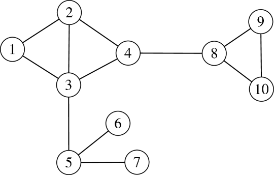
Figure 1: A simple graph with a tree-like subgraph: vertices 5, 6 and 7. Our graph figures are drawn using VISONE (www.visone.de).

Figure 2: The community structure of graph in Fig. 1 is depicted as a hierarchical tree or dendrogram with the complete linkage method for the similarity matrix $D$. Our dendrogram figures are drawn with the data plotting package and programming language R (http://www.R-project.org).

4.3 Zachary karate club network

To illustrate further the meaning of transient classes on $G(V,E)$ from global information carried out by ${\bf D}$ we analyze two well known networks in the literature.

The first example (Fig. 3) corresponds to the network of members of the karate club studied by Zachary Zachary . This graph contains a single leaf: member 12. Our analysis led to the hierarchical structure shown in Fig. 4 by means of a hierarchical clustering tree, defining communities at different levels. The two main communities reproduce exactly the observed splitting of the Zachary club and studied by different community finding techniques NewmanPRE69 ; NewmanEPJB04 ; Arenas05 ; HubermanEPJB38 ; Munoz04 ; Loreto04 ; NewmanPRE6904 ; Zhou_hier . Interestingly, a smaller community presented by the hierarchical tree can be clearly identified in Fig. 3. It consists of members displayed with shaded circles. This small group is only influenced by its members and has a direct interaction with the instructor.

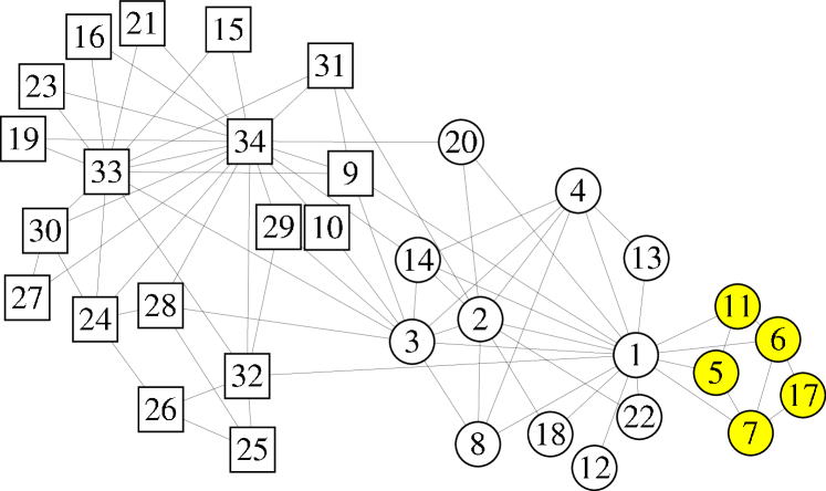
Figure 3: The karate club network studied by Zachary. Individual numbers represent the members of the club and edges their relationships as observed outside the normal activities of the club. Squares and circles indicate the observed final splitting of the karate club into two communities led by the administrator (34) and the instructor (1). A clear further splitting is identified with shaded circles.

Figure 4: The hierarchical structure of network in Fig. 3 is shown as a dendrogram with the complete linkage method. It correctly identifies the two main communities of the karate club.

4.4 Ravasz and Barabási square hierarchical network

The second example is shown in Fig. 5. It was designed by Ravasz and Barabási Barabasi03 as a prototype of hierarchical organization we may encounter in real network with scale-free topology and high modularity. The main figure is built with the module in (a). A similar figure but with more connections between vertices can be built with the module in (b). The study of $D_{ij}$ reveals community structures at different hierarchical levels in Fig. 6, respectively for the graphs generated with the modules (a) and (b).

The hierarchical trees present similar structures, but the hierarchical levels in both figures clearly display different network formation patterns. Moreover, the hierarchical formation pattern of $G(V,E)$ with branches at different heights may be seen as a measure of how cohesive those subgroups are. The normalized scale for $D_{ij}$ then can be used to also set degrees of cohesiveness related to the community formation.

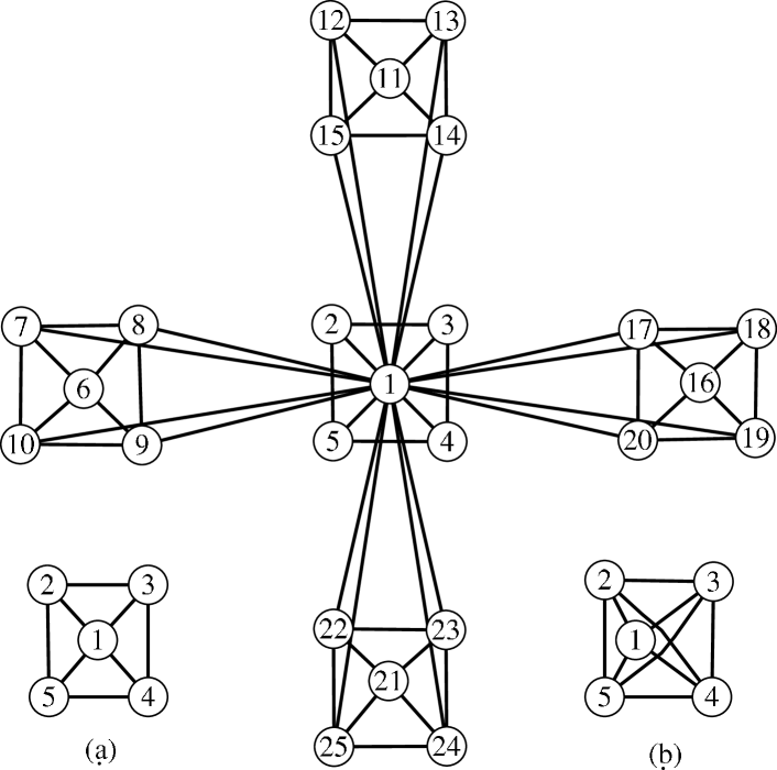
Figure 5: The deterministic hierarchical scale-free model with $n=5$ vertices proposed by Ravasz et al. Barabasi02 . It is built by generating replicas of the small 5-vertex module (a) shown at left side.

Figure 6: Hierarchical structure for the formation pattern of the network in Fig. 5. Dendrogram (a) refers to the network built with module (a) in Fig. 5 whereas dendrogram (b) refers to the graph built with module (b) in Fig.5.

5 WEIGHTS ON THE EDGES

Our method also applies to graphs such that each edge has a positive real number, the weight of the edge. The structure of the graph is now represented by the corresponding weighted adjacency matrix $\bf W$. It assigns weight $w_{ij}>0$ if and only if $i$ and $j$ are connected vertices and 0, otherwise. The concept of the Laplacian matrix extends directly to weighted edges, ${\bf L}(G)={\bf E}(G)-{\bf W}(G)$, where $E_{ii}=\sum_{j=1}^{n}w_{ij}$ is the diagonal weighted matrix whose values are the total weight of the edges adjacents to vertex $i$. Again, ${\bf L}(G)$ is a real symmetric matrix where the row sums and the column sums are all zero. Thus, we have the same spectral properties as recalled to the particular case $w_{ij}=1$ for all adjacent vertices $i$ and $j$. Therefore, the method presented to unweighted graphs extends naturally to weighted ones with no change in the algorithm.

5.1 Performance on artificial community weighted graphs

We have also verified the performance of this method on weighted graphs with fixed community structure NewmanE70W . Our test is performed on the same artificial graphs randomly generated as described in Section 4.A. The computer generated graphs have 128 vertices and are divided into four groups of 32 vertices. Here, edges among vertices are randomly chosen such that the average degree is fixed at 16. The test is performed for the most difficult situation where $z_{out}=z_{in}=8$. That is, each vertex has as many adjacent connections to inside as to outside its community. For each graph, we attach a weight $w>1$ to the edges inside each community and keep the fixed weight 1 for those edges which lie between communities. We evaluate again the fraction of vertices classified correctly as a function of $w$. As $w$ increases from the starting value 1, the weights enhance the community structure. This is clearly highlighted by our method. Our performance amounts to the following fractions of correctly classified vertices, $0.89,0.94,0.97$ and 0.98, respectively for $w=1.4,1.6,1.8$ and 2. The averages were calculated over 100 randomly generated graphs, with error bars smaller than 0.01.

5.2 identifying cohesive subgroups

As an example, we apply our method to the problem of analyzing weighted interactions related to verify how pairs of teachers are engaged in professional discussions Frank96 . This is a social network with $n=24$ members. Their edges are characterized by the professional discussions in a high school, called “Our Hamilton High”, during the 1992-1993 school year. Teachers were asked to list and weight the frequency of their discussions in that school to at most five teachers. This way of attributing weights leads to a directed network. The weights should follow a scale running from 1, for discussions occuring less than once a month, to the largest weight value 4, for almost daily discussions Frank96 . Every vertex number contains characteristics of teachers as gender, race, subject field, room assignment, among others. To perform our analysis we have defined the weights to each edge as the average of the values placed on the edges in the original directed network. Thus, this new weighted network is characterized by edges with real values in the range $(0.5,4)$ as representing the interactions among the members of that school. The community structure revealed by our analysis is represented by the dendrogram in Fig. 7. Its structure exhibits the formation of various communities. For comparison with the results in Frank96 , we also pick out the four main groups. The study of the their members reveals an association mainly according to race and gender, as also found in Ref. Frank96 . However, there are some differences in the members identification in each group. This may be due to the fact we are not analyzing exactly the same weighted network: our network is made undirect throught out an average process while the original one was handled in its original directed form.

Figure 7: Network community of professional discussions among teachers at “Our Hamilton High”.

6 Conclusions

In conclusion, random walks on graphs in connection with electrical networks highlight a topological property of $G(V,E)$: transient classes of vertices which we interpret as communities in the original graph. Here we emphasize that those special classes of vertices are a direct consequence of effective transition probabilities, which display a global perspective about the map of interactions that characterize the graph. We demonstrate its high performance in identifying community structures in some examples which became benchmark for initial algorithm validation. Moreover, it is parameter tunning independent. Our criterion to define communities depends only on $G(V,E)$ and not on any explicit definition of what a community structure must be.

It is likely that our proposed algorithm may produce new insights for large graphs. Application examples may include protein-protein interactions and the compartment identification in food-web structures. The visual information about how members form communities along the hierarchical tree may permit understand and characterize cohesive communities.

Acknowledgments

The author acknowledges valuable discussions with O. Kinouchi, A.S. Martinez and the support from the Brazilian agencies CNPq (303446/2002-1) and FAPESP (2005/04067-6).

References

- (1) A.-L. Barabási, Nature Phys. 1, 68 (2005).
- (2) R. Albert and A.-L. Barabási, Rev. Mod. Phys. 74, 47 (2002).
- (3) S.N. Dorogovtsev and J.F.F. Mendes, Adv. Phys. 51, 1079 (2002).
- (4) M.E.J. Newman, SIAM Review 45, 167 (2003).
- (5) P. Holme, M. Huss and H. Jeong, Bioinformatics 19, 532 (2003).
- (6) E. Ravasz, A.L. Somera, D.A. Mongru, Z.N. Oltvai and A.-L. Barabási, Science 297, 1551 (2002).
- (7) R. Guimerà and L.A.N. Amaral, Nature 433 895 (2005).
- (8) M. Vendruscolo, N.V. Dokholyan, E. Paci and M. Karplus, Phys. Rev. E 65, 061910 (2002).
- (9) L.H. Greene and V.A. Higman, J. Mol. Biol. 334, 781 (2003).
- (10) A.R. Atilgan, P. Akan and C. Baysal, Biophys. J. 86, 85 (2004).
- (11) N.A. Alves and A.S. Martinez, Physica A 375 336 (2007).
- (12) M.E.J. Newman, Eur. Phys. J. B. 38, 321 (2004).
- (13) L. Danon, A. Diaz-Guilera, J. Duch and A. Arenas, J. Stat. Mech. P09008 (2005).
- (14) M.E.J. Newman and M. Girvan, Phys. Rev. E 69, 026113 (2004).
- (15) F. Wu, B.A. Huberman, Eur. Phys. J. B 38, 331 (2004).
- (16) M.E.J. Newman, Phys. Rev. E 74 036104 (2006).
- (17) L. Donetti and M. A. Muñoz, J. Stat. Mech. P10012 (2004).
- (18) F. Radicchi, C. Castellano, F. Cecconi, V. Loreto and D. Parisi, Proc. Natl. Acad. Sci. USA 101 2658 (2004); C. Castellano, F. Cecconi, V. Loreto, D. Parisi, and F. Radicchi, Eur. Phys. J. B 38, 311 (2004);
- (19) W.W. Zachary, J. Anthropological Research 33, 452 (1977).
- (20) E. Ravasz and A.-L. Barabási, Phys. Rev. E 67, 026112 (2003).
- (21) R. Grone, Linear Algebra Appl. 150, 167 (1991) and references therein.
- (22) S.L. Campbell and C.D. Meyer, Generalized Inverses of Linear Transformations. Dover Publications, New York (1991).
- (23) A. Baltz and L. Kliemann, Lecture Notes in Computer Science 3418, 373 (2005).
- (24) K.M. Hall, Manag. Sci. 17, 219 (1970).
- (25) B. Bollobás, Modern Graph Theory, Springer-Verlag, New York 1998.
- (26) P.G. Doyle and J.L. Snell, Random walks and electric networks, Mathematical Association of America, 1999. (http://math.dartmouth.edu/ doyle/docs/walks/walks.ps)
- (27) W. Xiao and I. Gutman, Theor. Chem. Acc. 110, 284 (2003).
- (28) I. Gutman and W. Xiao, Bulletin de l’Academie Serbe des Sciences et des Arts (Cl. Math. Natur.) 129, 15 (2004).
- (29) M.E.J. Newman, Phys. Rev. E 69, 066133 (2004).
- (30) H. Zhou, Phys. Rev. E 67, 061901 (2003).
- (31) M.E.J. Newman, Phys. Rev. E 70, 056131 (2004).
- (32) K.A. Frank, Social Networks 18, 93 (1996).