Multiscale modeling of biopolymer translocation through a nanopore

Abstract

We employ a multiscale approach to model the translocation of biopolymers through nanometer size pores. Our computational scheme combines microscopic Langevin molecular dynamics (MD) with a mesoscopic lattice Boltzmann (LB) method for the solvent dynamics, explicitly taking into account the interactions of the molecule with the surrounding fluid. Both dynamical and statistical aspects of the translocation process were investigated, by simulating polymers of various initial configurations and lengths. For a representative molecule size, we explore the effects of important parameters that enter in the simulation, paying particular attention to the strength of the molecule-solvent coupling and of the external electric field which drives the translocation process. Finally, we explore the connection between the generic polymers modeled in the simulation and DNA, for which interesting recent experimental results are available.

1 Introduction

Biological systems exhibit a complexity and diversity far richer than the simple solid or fluid systems traditionally studied in physics or chemistry. The powerful quantitative methods developed in the latter two disciplines to analyze the behavior of prototypical simple systems are often difficult to extend to the domain of biological systems. Advances in computer technology and breakthroughs in simulational methods have been constantly reducing the gap between quantitative models and actual biological behavior. The main challenge remains the wide and disparate range of spatio-temporal scales involved in the dynamical evolution of complex biological systems. In response to this challenge, various strategies have been developed recently, which are in general referred to as “multiscale modeling”. These methods are based on composite computational schemes in which information is exchanged between the scales.

We have recently developed a multiscale framework which is well suited to address a class of biologically related problems. This method involves different levels of the statistical description of matter (continuum and atomistic) and is able to handle different scales through the spatial and temporal coupling of a mesoscopic fluid solvent, using the lattice Boltzmann method [1] (LB), with the atomistic level, which employs explicit molecular dynamics (MD). The solvent dynamics does not require any form of statistical ensemble averaging as it is represented through a discrete set of pre-averaged probability distribution functions, which are propagated along straight particle trajectories. This dual field/particle nature greatly facilitates the coupling between the mesoscopic fluid and the atomistic level, which proceeds seamlessy in time and only requires standard interpolation/extrapolation for information-transfer in physical space. Full details on this scheme are reported in Ref. [2]. We must note that to the best of our knowledge, although LB and MD with Langevin dynamics have been coupled before [3], this is the first time that such a coupling is put in place for long molecules of biological interest.

Motivated by recent experimental studies, we apply this multiscale approach to the translocation of a biopolymer through a narrow pore. These kind of biophysical processes are important in phenomena like viral infection by phages, inter-bacterial DNA transduction or gene therapy [4]. In addition, they are believed to open a way for ultrafast DNA-sequencing by reading the base sequence as the biopolymer passes through a nanopore. Experimentally, translocation is observed in vitro by pulling DNA molecules through micro-fabricated solid state or membrane channels under the effect of a localized electric field [5]. From a theoretical point of view, simplified schemes [6] and non-hydrodynamic coarse-grained or microscopic models [7, 8] are able to analyze universal features of the translocation process. This, though, is a complex phenomenon involving the competition between many-body interactions at the atomic or molecular scale, fluid-atom hydrodynamic coupling, as well as the interaction of the biopolymer with wall molecules in the region of the pore. A quantitative description of this complex phenomenon calls for state-of-the art modeling, towards which the results presented here are directed.

2 Numerical Set-up

In our simulations we use a three-dimensional box of size $N_{x}\times N_{x}/2\times N_{x}/2$ in units of the lattice spacing $\Delta x$. The box contains both the polymer and the fluid solvent. The former is initialized via a standard self-avoiding random walk algorithm and further relaxed to equilibrium by Molecular Dynamics. The solvent is initialized with the equilibrium distribution corresponding to a constant density and zero macroscopic speed. Periodicity is imposed for both the fluid and the polymer in all directions. A separating wall is located in the mid-section of the $x$ direction, at $x/\Delta x=N_{x}/2$, with a square hole of side $h=3\Delta x$ at the center, through which the polymer can translocate from one chamber to the other. For polymers with up to $N=400$ beads we use $N_{x}=80$; for larger polymers $N_{x}=100$. At $t=0$ the polymer resides entirely in the right chamber at $x/\Delta x>N_{x}/2$. The polymer is advanced in time according to the following set of Molecular Dynamics-Langevin equations for the bead positions $\vec{r}_{p}$ and velocities $\vec{v}_{p}$ (index $p$ runs over all beads):

$$M_{p}\frac{d\vec{v}_{p}}{dt} = -\sum_{q}\partial_{\vec{r}_{p}}V_{LJ}(\vec{r}_{p}-\vec{r}_{q})+\gamma(\vec{u}_{p}-\vec{v}_{p})+M_{p}\vec{\xi}_{p}-\lambda_{p}\partial_{\vec{r}_{p}}\kappa_{p}$$ (1)

These interact among themselves through a Lennard-Jones potential with $\sigma=1.8$ and $\varepsilon=10^{-4}$:

$$V_{LJ}(r)=4\varepsilon\left[\left(\frac{\sigma}{r}\right)^{12}-\left(\frac{\sigma}{r}\right)^{6}\right]$$ (2)

This potential is augmented by an angular harmonic term to account for distortions of the angle between consecutive bonds. The second term in Eq.(1) represents the mechanical friction between a bead and the surrounding fluid, $\vec{u}_{p}$ is the fluid velocity evaluated at the bead position and $\gamma$ the friction coefficient. In addition to mechanical drag, the polymer feels the effects of stochastic fluctuations of the fluid environment, through the random term, $\vec{\xi}_{p}$. This is related to the third term in Eq.(1), which is an incorrelated random term with zero mean. Finally, the last term in Eq.(1) is the reaction force resulting from $N-1$ holonomic constraints for molecules modelled with rigid covalent bonds. The bond length is set at $b=1.2$ and $M_{p}$ is the bead mass equal to 1.

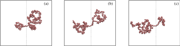
Figure 1: Snapshots of a typical event: a polymer ($N=300$) translocating from the right to the left is depicted at a time equal to (a) 0.11, (b) 0.47, and (c) 0.81 of the total time for this translocation. The vertical line in the middle of each panel shows the wall.

Translocation is induced by a constant electric force ($F_{drive}$) which acts along the $x$ direction and is confined in a rectangular channel of size $3\Delta x\times\Delta x\times\Delta x$ along the streamwise ($x$ direction) and cross-flow ($y,z$ directions). The solvent density and kinematic viscosity are $1$ and $0.1$, respectively, and the temperature is $k_{B}T=10^{-4}$. All parameters are in units of the LB timestep $\Delta t$ and lattice spacing $\Delta x$, which we set equal to 1. Additional details have been presented in Ref. [2]. In our simulations we use $F_{drive}=0.02$ and a friction coefficient $\gamma=0.1$. It should be kept in mind that $\gamma$ is a parameter governing both the structural relation of the polymer towards equilibrium and the strength of the coupling with the surrounding fluid. The MD timestep is a fraction of the timestep for the LB part $\Delta t=m\Delta t_{MD}$, where $m$ is a constant typically set at $m=5$. With this parametrization, the process falls in the fast translocation regime, where the total translocation time is much smaller than the Zimm relaxation time. We refer to this set of parameters as our “reference”; we explore the effect of the most important parameters for certain representative cases.

3 Translocation dynamics

Extensive simulations of a large number of translocation events over $100-1000$ initial polymer configurations for each length confirm that most of the time during the translocation process the polymer assumes the form of two almost compact blobs on either side of the wall: one of them (the untranslocated part, denoted by $U$) is contracting and the other (the translocated part, denoted by $T$) is expanding. Snapshots of a typical translocation event shown in Fig. 1 strongly support this picture. A radius of gyration $R_{I}(t)$ (with $I=U,T$) is assigned to each of these blobs, following a static scaling law with the number of beads $N_{I}$: $R_{I}(t)\sim N_{I}^{\nu}(t)$ with $\nu\simeq 0.6$ being the Flory exponent for a three-dimensional self-avoiding random walk. Based on the conservation of polymer length, $N_{U}+N_{T}=N_{tot}$, an effective translocation radius can be defined as $R_{E}(t)\equiv(R_{T}(t)^{1/\nu}+R_{U}(t)^{1/\nu})^{\nu}$. We have shown that $R_{E}(t)$ is approximately constant for all times when the static scaling applies, which is the case throughout the process except near the end points (initiation and completion of the event) [2]. At these end points, deviations from the mean field picture, where the polymer is represented as two uncorrelated compact blobs, occur. The volume of the polymer also changes after its passage through the pore. At the end, the radius of gyration is considerably smaller than it was initially: $R_{T}(t_{X})<R_{U}(0)$, where $t_{X}$ is the total translocation time for an individual event. For our reference simulation an average over a few hundreds of events for $N=200$ beads showed that $\lambda_{R}=R_{T}(t_{X})/R_{U}(0)\sim 0.7$. This reveals the fact that as the polymer passes through the pore it is more compact than it was at the initial stage of the event, due to incomplete relaxation.

The variety of different initial polymer realizations produce a scaling law dependence of the translocation times on length [8]. By accumulating all events for each length, duration histograms were constructed. The resulting distributions deviate from simple gaussians and are skewed towards longer times (see Fig. 2(a) inset). Hence, the translocation time for each length is not assigned to the mean, but to the most probable time ($t_{max}$), which is the position of the maximum in the histogram (noted by the arrow in the inset of Fig. 2(a) for the case $N=200$). By calculating the most probable times for each length, a superlinear relation between the translocation time $\tau$ and the number of beads $N$ is obtained and is reported in Fig. 2(a). The exponent in the scaling law $\tau(N)\sim N^{\alpha}$ is calculated as $\alpha\sim 1.28\pm 0.01$, for lengths up to $N=500$ beads. The observed exponent is in very good agreement with a recent experiment on double-stranded DNA translocation, that reported $\alpha\simeq 1.27\pm 0.03$ [9]. This agreement makes it plausible that the generic polymers modeled in our simulations can be thought of as DNA molecules; we return to this issue in section 5.

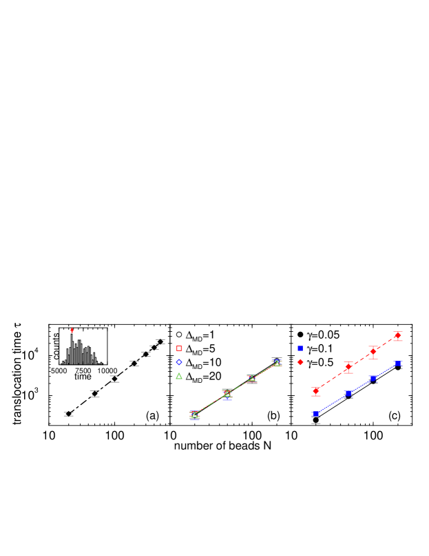
Figure 2: (a) Scaling of $\tau$ with the number of beads $N$. Inset: distribution of translocation times over 300 events for $N=200$. Time is given in units of the LB timestep. The arrow shows the most probable translocation time for this length. Effect of the various parameters on the scaling law: (b) changing the value of the MD timestep ($\Delta t_{MD}$); (c) changing the value of the solvent-molecule coupling coefficient $\gamma$.

4 Effects of parameter values

We next investigate the effect that the various parameters have on the simulations, using as standard of comparison the parameter set that we called the “reference” case. For all lengths and parameters about 100 different initial configurations were generated to assess the statistical and dynamical features of the translocation process. As a first step we simulate polymers of different lengths ($N=20-200$). Following a procedure similar to the previous section we extract the scaling laws for the translocation time and their vatiation with the friction coefficient $\gamma$ and the MD timestep $\Delta t_{MD}$. The results are shown in Fig. 2(b) and (c). In these calculations the error bars were also taken into account. The scaling exponent for our reference simulation ($\gamma=0.1$) presented in Fig. 2(a) is $\alpha\simeq 1.27\pm 0.01$ when only the lengths up to $N=200$ are included. The exponent for smaller damping ($\gamma=0.05$) is $\alpha\simeq 1.32\pm 0.06$, and for larger ($\gamma=0.5$) $\alpha\simeq 1.38\pm 0.04$. By increasing $\gamma$ by one order of magnitude the time scale rises by approximately one order of magnitude, showing an almost linear dependence of the translocation time with hydrodynamic friction; we discuss this further in the next section. However, for larger $\gamma$, thus overdamped dynamics and smaller influence of the driving force, the deviation from the $\alpha=1.28$ exponent suggests a systematic departure from the fast translocation regime. Similar analysis for various values of $\Delta t_{MD}$ shows that the exponent becomes $\alpha\simeq 1.34\pm 0.04$ when $\Delta t_{MD}$ is equal to the LB timestep ($m=1$); for $m=10$ the exponent is $\alpha\simeq 1.32\pm 0.04$, while for $m=20$, $\alpha\simeq 1.28\pm 0.01$ with similar prefactors.

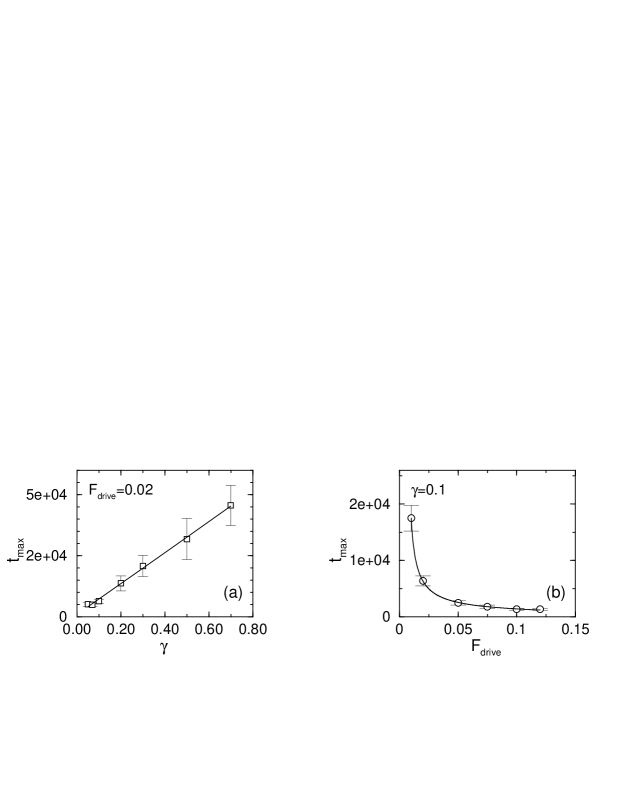
Figure 3: Variation of $t_{max}$ with (a) $\gamma$, and (b) $F_{drive}$ for $N=200$ beads.

We next consider what happens when we fix the length to $N=200$ and vary $\gamma$ and the pulling force $F_{drive}$. For all forces used, the process falls in the fast translocation regime. The most probable time ($t_{max}$) for each case was calculated and the results are shown in Fig. 3. The dependence of $t_{max}$ on $\gamma$ is linear related to the linear dependence of $\tau$ on $\gamma$, mentioned in the previous section. The variation of $t_{max}$ with $F_{drive}$ follows an inverse power law: $t_{max}\sim 1/F_{drive}^{\mu}$, with $\mu$ of the order 1. The effect of $\gamma$ is further explored in relation to the effective radii of gyration $R_{E}$, and is presented in Fig. 4. The latter must be constant when the static scaling $R\sim N^{0.6}$ holds. This is confirmed for small $\gamma$ up to about $0.2$. As $\gamma$ increases, $R_{E}$ is no more constant with time, and shows interesting behavior: it increases continuously up to a point where a large fraction of the chain has passed through the pore and subsequently drops to a value smaller than the initial $R_{U}(0)$. Hence, as $\gamma$ increases large deviations from the static scaling occur and the translocating polymer can no longer be represented as two distinct blobs. In all cases, the translocated blob becomes more compact. For all values of $\gamma$ considered, $\lambda_{R}$ is always less than unity ranging from $0.7$ ($\gamma$=0.1) to $0.9$ ($\gamma$=0.5) following no specific trend with $\gamma$.

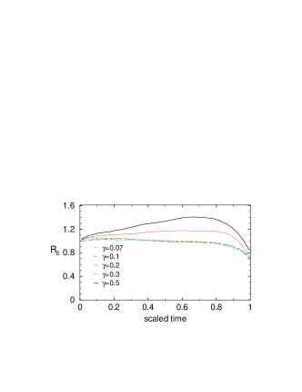
Figure 4: The dependence of the effective radii of gyration $R_{E}(t)$ on $\gamma$ ($N=200$). Time and $R_{E}$ are scaled with respect to the total translocation time and $R_{U}(0)$ for each case.

5 Mapping to real biopolymers

As a final step towards connecting our computer simulations to real experiments and after having established the agreement in terms of the scaling behavior, we investigate the mapping issue of the polymer beads to double-stranded DNA. In order to interpret our results in terms of physical units, we turn to the persistence length ($l_{p}$) of the semiflexible polymers used in our simulations. Accordingly, we use the formula for the fixed-bond-angle model of a worm-like chain [10]:

$$l_{p}=\frac{b}{1-\cos\langle\theta\rangle}$$ (3)

where $\langle\theta\rangle$ is complementary to the average bond angle between adjacent bonds. In lattice units ($\Delta x$) an average persistence length for the polymers considered, was found to be approximately $12$. For $\lambda$-phage DNA $l_{p}\sim 50$ nm [11] which is set equal to $l_{p}$ for our polymers. Thereby, the lattice spacing is $\Delta x\sim 4$ nm, which is also the size of one bead. Given that the base-pair spacing is $\sim 0.34$ nm, one bead maps approximately to $12$ base pairs. With this mapping, the pore size is about $\sim 12$ nm, close to the experimental pores which are of the order of $10$ nm. The polymers presented here correspond to DNA lengths in the range $0.2-6$ kbp. The DNA lengths used in the experiments are larger (up to $\sim$ 100kbp); the current multiscale approach can be extended to handle these lengths, assuming that appropriate computational resources are available.

Choosing polymer lengths that match experimental data we compare the corresponding experimental duration histograms (see Fig. 1c of Ref. [9]) to the theoretical ones. This comparison sets the LB timestep to $\Delta t\sim 8$ nsec. In Fig. 5 the time distributions for representative DNA lengths simulated here are shown. In this figure, physical units are used according to the mapping described above and promote comparison with similar experimental data [9]. The MD timestep for $m=5$ will then be $t_{MD}\sim 40$ nsec indicating that the MD timescale related to the coarse-grained model that handles the DNA molecules is significantly stretched over the physical process. Exact match to all the experimental parameters is of course not feasible with coarse-grained simulations. However, essential features of DNA translocation are captured, allowing the use of the current approach to model similar biophysical processes that involve biopolymers in solution. This can become more efficient by exploiting the freedom of further fine-tuning the parameters used in this multiscale model.

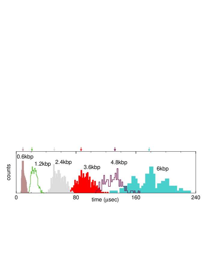
Figure 5: Histograms of calculated translocation times for a large number of events and different DNA lengths. The arrows link to the most probable time ($t_{max}$) for each case.

6 Conclusions

In summary, we applied a multiscale methodology to model the translocation of a biopolymer through a nanopore. Hydrodynamic correlations between the polymer and the surrounding fluid have explicitly been included. The polymer obeys a static scaling except near the end points for each event (initiation and completion of the process) and the translocation times vary exponentially with the polymer length. A preliminary exploration of the effects of the most important parameters used in our simulations was also presented, specifically the values of the friction coefficient and the pulling force describing the effect of the external electric field that drives the translocation. These were found to significantly affect the dynamic features of the process. Finally, our generic polymer models were directly mapped to double-stranded DNA and a comparison to experimental results was discussed.

Acknowledgments.

MF acknowledges support by Harvard’s Nanoscale Science and Engineering Center, funded by NSF (Award No. PHY-0117795).

References

- [1] Wolf-Gladrow, D. A.: Lattice gas cellular automata and lattice Boltzmann models. Springer Verlag, New York 2000; Succi, S.: The lattice Boltzmann equation. Oxford University Press, Oxford 2001; Benzi, R. Succi, S., and Vergassola, M.:, The lattice Boltzmann-equation - Theory and applications. Phys. Rep. 222 (1992) 145–197.
- [2] Fyta, M. G., Melchionna, S., Kaxiras, E., and Succi, S.: Multiscale coupling of molecular dynamics and hydrodynamics: application to DNA translocation through a nanopore. Multiscale Model. Simul. 5 (2006) 1156–1173.
- [3] Ahlrichs, P. and Duenweg, B.: Lattice-Boltzmann simulation of polymer-solvent systems. Int. J. Mod. Phys. C 9 (1999) 1429–1438; Simulation of a single polymer chain in solution by combining lattice Boltzmann and molecular dynamics. J. Chem. Phys. 111 (1999) 8225–8239.
- [4] Lodish, H., Baltimore, D., Berk, A., Zipursky, S., Matsudaira, P., and Darnell, J.: Molecular Cell Biology, W.H. Freeman and Company, New York (1996).
- [5] Kasianowicz, J. J., et al: Characterization of individual polynucleotide molecules using a membrane channel. Proc. Nat. Acad. Sci. USA 93 (1996) 13770–13773; Meller, A., et al: Rapid nanopore discrimination between single polynucleotide molecules. 97 (2000) 1079–1084; Li, J., et al: DNA molecules and configurations in a solid-state nanopore microscope. Nature Mater. 2 (2003) 611–615.
- [6] Sung, W. and Park, P. J.: Polymer translocation through a pore in a membrane. Phys. Rev. Lett. 77 (1996) 783–786.
- [7] Matysiak, S., et al: Dynamics of polymer translocation through nanopores: Theory meets experiment. Phys. Rev. Lett. 96 (2006) 118103.
- [8] Lubensky, D. K. and Nelson, D. R.: Driven polymer translocation through a narrow pore. Biophys. J. 77 (1999) 1824–1838.
- [9] Storm, A. J. et al: Fast DNA translocation through a solid-state nanopore. Nanolett. 5 (2005) 1193–1197.
- [10] Yamakawa, H.: Modern Theory of Polymer Solutions, Harper & Row, NY 1971.
- [11] Hagerman, P. J.: Flexibility of DNA. Annu. Rev. Biophys. Biophys. Chem. 17 (1988) 265–286; Smith, S., Finzi, L., and Bustamante, C.: Direct mechanical measurement of the elasticity of single DNA molecules by using magnetic beads. Science 258 (1992), 1122–1126.