Automatic Reconstruction of Fault Networks from Seismicity Catalogs: 3D Optimal Anisotropic Dynamic Clustering

Abstract

We propose a new pattern recognition method that is able to reconstruct the $3D$ structure of the active part of a fault network using the spatial location of earthquakes. The method is a generalization of the so-called dynamic clustering method, that originally partitions a set of datapoints into clusters, using a global minimization criterion over the spatial inertia of those clusters. The new method improves on it by taking into account the full spatial inertia tensor of each cluster, in order to partition the dataset into fault-like, anisotropic clusters. Given a catalog of seismic events, the output is the optimal set of plane segments that fits the spatial structure of the data. Each plane segment is fully characterized by its location, size and orientation. The main tunable parameter is the accuracy of the earthquake localizations, which fixes the resolution, i.e. the residual variance of the fit. The resolution determines the number of fault segments needed to describe the earthquake catalog, the better the resolution, the finer the structure of the reconstructed fault segments. The algorithm reconstructs successfully the fault segments of synthetic earthquake catalogs. Applied to the real catalog constituted of a subset of the aftershocks sequence of the 28th June 1992 Landers earthquake in Southern California, the reconstructed plane segments fully agree with faults already known on geological maps, or with blind faults that appear quite obvious on longer-term catalogs. Future improvements of the method are discussed, as well as its potential use in the multi-scale study of the inner structure of fault zones.

OUILLON, DUCORBIER and SORNETTE 3D determination of fault patterns Guy Ouillon, Lithophyse, 1 rue de la croix, 06300 Nice, France (e-mail: lithophyse@free.fr) Caroline Ducorbier, LPMC, CNRS and University of Nice, 06108 Nice, France () Didier Sornette, D-MTEC, ETH Zurich, Kreuzplatz 5, CH-8032 Zurich, Switzerland and D-ESS and IGPP, UCLA, Los Angeles, California, USA (e-mail: dsornette@ethz.ch)

1 Introduction

Tectonic deformation encompasses a wide spectrum of scales, both in spatial and temporal dimensions. This certainly constitutes a fundamental obstacle to thoroughly study, from observations alone, the whole set of relevant processes. It is now clear that seismic events occur on faults, while faults grow by accumulation of slip, by the growth of damage in the region of their tips, and by linkage between pre-existing faults of various sizes, all three processes occuring in large part during earthquakes (see Scholz (2002) for a review of earthquake nucleation and fault growth mechanisms and Sornette et al. (1990) and Sornette (1991) for a general theoretical set-up). In the last twenty years, a large amount of knowledge has been obtained on the statistical properties and general phenomenology of faults and earthquakes (including the distribution of sizes, of inter-event time distributions, the geometrical correlations, and so on), but a clear physical and mechanical understanding of the links and interactions between and among them is still missing. Such knowledge may prove decisive to drastically improve our understanding of seismic risks, especially the time-dependent risks associated with the future large and potentially destructive seismic events.

The study of natural fault networks and of earthquake catalogs is generally conducted in two very different ways, which clearly reveal still distinct scientific cultures. On one side, brittle tectonics (within which we include seismotectonics) and structural geology pays a lot of attention to structures, but dwells quite little on their nonlinear collective dynamics. Thus, brittle tectonics and structural geology are incapable of any predictive seismological statement, despite an impressive amount of theoretical and laboratory-validated concepts coming from rock physics and rheology (see Scholz (2002), Passchier and Trouw (2005) and Pollard and Fletcher (2005)), as well as from observational techniques. Brittle tectonics and structural geology mainly consider structures as isolated and thus focus on the “one-body” problem, generally solvable through the use of classical physics and/or the use of the mechanics of homogeneous media. On the other side, statistical analyses can reveal patterns, but rarely provide anything else than purely empirical descriptions of the data. Some statistical analyses may even be seriously flawed due to their very nature (see for instance Ouillon and Sornette (1996) who reveal a mechanism leading to spurious multifractal analyses of fault patterns). For instance, when dealing with earthquakes, most spatial analyses deal with epicenters or hypocenters. Since real earthquakes involve extended oriented structures, statistical analyses based on point-wise representation of earthquakes may led to spurious correlations between events, especially the smallest ones, which may distord any model of the collective build-up of a large shock by previous smaller events.

Statistical analyses can also be performed using fault networks, but they are most often restricted to the available 2D surface maps. It is then difficult to assess the amount of information that is genuinely representative of 3D active faulting at depth and, as such, related to seismogenesis, in the goal of developing better understanding and improved forecasts. There are several problems when working with networks of surface-intersecting faults. First, the sampling of fault data is by far more difficult and time-consuming than constructing earthquake catalogs, with the often unavoidable existence of subjective inputs. Second, one can only map small-scale features in small-scale domains (see Ouillon et al (1995) and Ouillon et al (1996) for a rather unique high-resolution multi-scale analysis of fracturing and faulting of the Arabic plate). The domains chosen for such sampling may not be good representative, as their choice may either be arbitrary or reflect practical constraints. Third, there can exist some masks (like cities, deserts or vegetation) which make observations impossible in sometimes vast areas. This can seriously bias statistical results (see Ouillon and Sornette (1996)). In any case, if one takes account of all those shortcomings, spatial analyses are possible at any scale (from millimeters to thousands of kilometers - see Ouillon et al (1995) and Ouillon et al (1996) which showed how to exploit such data with multifractal and anisotropic wavelet methods so as to reconstruct objective fault maps at multiple scales), but there is a terrible lack of data in the time domain. Darrozes et al. (1998) and Gaillot et al. (2002) studied the aftershock sequence of the 1980 M5.1 Arudy earthquake in the French Pyrénées using anisotropic wavelets. Their method is an extension of the Optimal Anisotropic Wavelet Coefficient method (Ouillon et al (1995); Ouillon et al (1996)). This method uses anisotropic filters, which properties (size and orientation) can vary from one location to another within the same dataset. At each spatial location, the shape of the filter is chosen such that it reveals best the local anisotropic features, if any (hence the “optimal” qualification). In this way, each pixel in the image is characterized by a local optimal anisotropy. This method allowed one to detect and map linear structures in the Arudy sequence, and to quantify their orientation. However, identified faults are still sets of neighbouring pixels, each pixel “ignoring” that it possibly belongs to the same fault as its neighbours. The images provided by wavelet analysis still need to be post-processed in order to compute, for example, the size of the lineaments. The method is also restricted to 2D datasets. Extension to 3D geometries would be theoretically straightforward, but the size of images to handle at the scale of a regional catalogue is totally unrealistic, as large volumes of space would have to be discretized at scales much lower than the earthquake localization accuracy.

The structure of the present state of a fault pattern integrates its whole history, i.e. reflects the largest possible time scale, which can be several tens of millions of years. At very short time scales, seismology offers pictures of the slip pattern over a reconstructed fault surface that occured during an earthquake. But this kind of inversion is performed only for the largest shocks. In between, paleo-seismology allows one to decipher the sliding history along discontinuities, but it still focuses on major faults and major seismic events for obvious reasons of time and space resolution. In fact, there is absolutely no work at all on the mechanics of faulting within a fault network as a whole derived from field observations, at time scales comparable with those of a seismic catalog. Obtaining such information would certainly constrain significantly our concepts and methods on the space-time organization of earthquakes and on the potential for their forecasts, with the ultimate goal of better assessment of time-dependent hazard.

Most studies focus on earthquake catalogs. This comes from the fact that earthquake catalogs contain in general a large number of events, allowing accurate statistics to be computed, and that building such a database is reasonably mastered at the technical level. A homogeneous seismographic network can span a very large domain, which allow for spatial analyses at scales from a few tens of meters to hundreds or thousands of kilometers, at least in $2D$. Depth is often omitted in most statistical analyses, as the increases of pressure and temperature, as well as the finite thickness of the seismogenic layer, clearly break any possible symmetry along the vertical direction, which one generally does not know how to deal with when performing statistics (see however Béthoux et al (1998) for a genuine 3D wavelet analysis of seismicity in the Alpine arc). Another reason for the use of seismic catalogs for the analysis of fault networks is that they also allow for clean analyses in the time domain, at scales varying from few seconds to decades.

Up to now, most of the information available on the structure of fault patterns comes from surface mapping at various scales. One can however question the reliability of such data sets, as earthquakes catalogs generally include large quantities of events which do not seem to be linked to any such faults, but rather seem to be associated with active faults buried at depth which do not cross-cut the surface. It is thus rather clear that comparing $2D$ map views of the long-term cumulative brittle deformation to the $3D$ structure of the short-term incremental deformation can provide at best a poor insight into, and at worst a biased incorrect model of, the multi-scale tectonic processes as a whole. A detailed knowledge of the $3D$ structure of fault networks is needed to better understand the mechanics of earthquake interaction and collective behaviour. In the last few years, in parallel to the ever increasing capabilities of computers, earthquake localization algorithms have significantly improved so that the accuracy for the spatial resolution of earthquake hypocenters dropped down to about $1km$, and even to a few tens of meters within clusters (when using relative locations through cross-correlating waveforms, Shearer et al (2005)). This provides new opportunities to learn about the detailed $3D$ structure of fault patterns at depth using seismicity itself as a diagnostic.

The basis of our paper is that seismic hazard assessment faces two fundamental bottlenecks: (i) catalogs are inherently incomplete with respect to the typical recurrence time of large earthquakes which are many times larger than the duration of the available catalogs; (ii) earthquakes occur on faults, but most of them are still unknown, drastically limiting our understanding and our assessment of seismic risks. The principal issue therefore lies in the association between earthquakes and faults. A recent effort to assign earthquakes and simple fault structures in the San Francisco Bay area showed significant disparities that arose from the simplified geometry of fault zones at depth and the amount and direction of systematic biases in the calculation of earthquake hypocenters (Wesson, 2003). The geometry of an active fault zone is often constrained by mapping the surface trace; dip angle at depth and depth extent are either constrained by results of controlled source seismology (if available) and the distribution of hypocenter locations or they are just extrapolated using geometric constraints, if seismologic constraints are not available. For example, one of the most sophisticated fault models available, the Community Fault Model (CFM) of the Southern California Earthquake Center (SCEC), combines available information on surface traces, seismicity, seismic reflection profiles, borehole data, and other subsurface imaging techniques to provide three-dimensional representations of major strike-slip, blind-thrust, and oblique-reverse faults of southern California (Plesch, 2002). Each fault is represented by a triangulated surface in a precise geographic reference frame. However, the representation of a fault by a simple surface cannot reflect the fine-detailed structure seen in extinct fault zones and in drilling experiments of active faults (e.g. Scholz, 2002 ; Faulkner, 2003). These results suggest that fault zones actually consist of narrow earthquake-generating cores, possibly accompanied by small subsidiary faults. Our present contribution is to propose a general method to identify and locate active faults in seismically active regions by using a scientifically rigorous approach based on active seismicity. Our goal is to gain a better understanding of the link between fault structures and earthquakes.

For this, the present paper presents a new pattern recognition method which determines an optimal set of plane segments, hereafter labeled as ‘faults’ that best fit a given set of earthquake hypocenters. In the first part, we provide a short overview of pattern recognition methods used to detect linear or planar features in images, such as the Hough and wavelet transforms. We then present in more details the dynamic clustering method, which provides a partition of a set of data points into clusters, before detailing our new method, a generalization of dynamic clustering to the case of anisotropic structures. We illustrate this new technique through benchmark tests on synthetic datasets, before providing results obtained on a subset of the Landers aftershocks sequence. The final discussion of our results compares this new method with other clustering methods, and outline its potential use in the study of fault-zones structures. We then sketch the next set of improvements for this method which will be developed in sequel papers.

2 Line and plane detection in image analysis

The detection of linear and planar structures in seismotectonics has a long history, but still suffers from a lack of quantitative methods. From the early years of instrumental seismology, the main instrument to identify faults from earthquakes has indeed been the eye. It is by visual inspection that tectonic plates boundaries or the Benioff plane in subduction zones have been delineated. Visual inspection remains the main approach to identify blind faults at smaller scales. Very few efforts have been devoted to the development of automatic digital detections of linear or planar spatial features from earthquake catalogs. We shall thus now describe two major approaches in image analysis, and outline their advantages and drawbacks, before turning to dynamic clustering.

2.1 The Hough transform

The Hough transform (see Duda and Hart, 1972) is a technique that is widely used in digital image analysis, with applications, for example, in the detection and characterization of edges, or the reconstruction of trajectories in particle physics experiments. The original Hough transform identifies linear features within an image, but it can be extended to other shapes (like circles or ellipses). We shall anyway present it for straight line detection in $2D$ for the sake of simplicity. The basic idea is that, given a set of data points, there is an infinite number of lines that can pass through each point. The aim of the Hough transform is to determine the set of lines that get through several points.

Each line can be parameterized using two parameters $r$ and $\theta$ in the Hough space. The parameter $r$ is the distance between this line and the origin, and $\theta$ is the orientation of the normal to that line (and is measured from the abscissa axis). Then, the infinite number of lines passing through a given point defines a curve $r(\theta)$ in the Hough plane. All lines passing through a point located at $(x_{0},y_{0})$ obey the equation $r(\theta)=x_{0}\cdot\cos(\theta)+y_{0}\cdot\sin(\theta)$. If we now consider several points of our dataset that are located on the same straight line in direct space, their associated $r(\theta)$ curves will all cross at the same $(r,\theta)$ point in the Hough space. Reciprocally, the corresponding line is then fully identified. Note that several distinct sets of $r(\theta)$ curves can cross in the Hough space at different $(r,\theta)$ locations, so that as many linear features can be extracted at once. This idea can be extended to arbitrary $2D$ structures (such as circles or ellipses) or to 3D spaces and planar features, provided that one extends the dimension of the Hough space correspondingly. For example, this dimension is equal to $4$ when one wants to detect straight lines in a $3D$ real space, so that the method is not used in practice in that case (or rather in a much simplified form, provided there is only a very small number of such lines to detect, see Bhattacharya et al (2000)). The dimension of the Hough space drops to $3$ when dealing with planar features.

The main problem of this technique is that it does not provide directly the spatial extension of the linear or planar features, only their positions in space, as each line (or plane) has an infinite size. A post-processing step must then be performed in order to compute the finite extension. Another drawback is that the Hough transform does not take account of the uncertainties in the localization of the set of data points, a crucial parameter in seismology. All in all, it appears that the Hough transform is very efficient only when dealing with few very clean ordered patterns (see however some specific strategies that can be defined to deal with real fracture planes (Sarti and Tubaro, 2002). Another major argument against the use of the Hough transform for fault segment reconstruction from seismic catalogs is that there is absolutely no way to include any other information one may have about seismic events, such as their seismic moment tensors, focal mechanisms or magnitudes.

2.2 The Optimal Anisotropic Wavelet Coefficient method

The characterization of anisotropy is a basic task in structural geology, tectonics and seismology. The orientations of structures stem from mechanical boundary conditions, which we are in general interested to invert. They control the future evolution of the system, which we are interested to predict. Tools for quantifying anisotropy generally materialize in rose diagrams (for $2D$ fracture maps for instance) or in stereographical projections (when data are sampled in $3D$ space). The main drawback of these representations is that they are scale-dependent. For example, as shown in (Ouillon, 1995 ; Ouillon et al, 1995), in the case of en-échelon fractures, small-scale and large-scale features will possess fundamentally different anisotropy properties. In that case, mapping at small scales will not give any clue on the large scale properties of the system. The so-called Optimal Anisotropic Wavelet Coefficient (OAWC) method, presented in the above publications, was designed to specifically address this problem.

For $2D$ signals, such as fault maps and fracture maps, a wavelet is a band-pass filter which is characterized, in real space, by a width (called resolution), a length and an azimut. In a nutshell, the OAWC method consists in fixing the resolution and convolving the wavelet with the map of fault traces, varying its length and azimut. For any given position, when the result of the convolution (which is the wavelet coefficient) reaches a maximum, one stores the associated azimut of the wavelet and switch to the next spatial location. Building a histogram of such optimal azimuts provides a rose diagram at the considered resolution. Performing this process at different resolutions allows one to describe the evolution of anisotropy with scale from a single initial data set. Looking at various maps of fractures and faults patterns in Saoudi Arabia, Ouillon, 1995 and Ouillon et al, 1995 were able to show that anisotropy properties change drastically at resolutions that can be related to the thicknesses of the mechanical layers involved in the brittle deformation process (from sandstone beds up to the continental crust).

The OAWC method has been extended to characterize the anisotropy of mineralization in thin plates, as well as to detect faults or lineaments from earthquakes epicenter maps (Darrozes et al, 1997 ; Darrozes et al, 1998 ; Gaillot et al, 1997 ; Gaillot et al, 1999 ; Grégoire et al, 1998). In this second class of applications, the issue concerning the finite accuracy of event localizations is addressed by considering a wavelet resolution larger than the spatial uncertainties. However, this method does not provide direct information about the size of the structures, and indeed does not manipulate structures as such. Each point in space is characterized by anisotropy properties, but the method do not naturally construct clusters from neighbouring points with similar characteristics. Moreover, its extension to $3D$ signals and their associated 3D patterns would prove unreasonably time-consuming (as space has to be discretized at a scale smaller than the chosen resolution) and would suffer from edge effects near the top and bottom of the seismogenic zone. Nothwithstanding its power and flexibility, it is no better that the Hough transform for our present problem of reconstructing a network of fault segments best associated with a given seismic catalog.

3 Dynamic clustering

3.1 Dynamic clustering in 2D

Dynamic clustering (also known as k-means) is a very general image processing technique that allows one to partition a set of data points using a simple criterion of inertia. The method is described in many papers or textbooks (see for example Mac Queen (1967)), so it will suffice for our purposes to perform a practical demonstration in $2D$ - but extension of the method to $3D$ is straightforward.

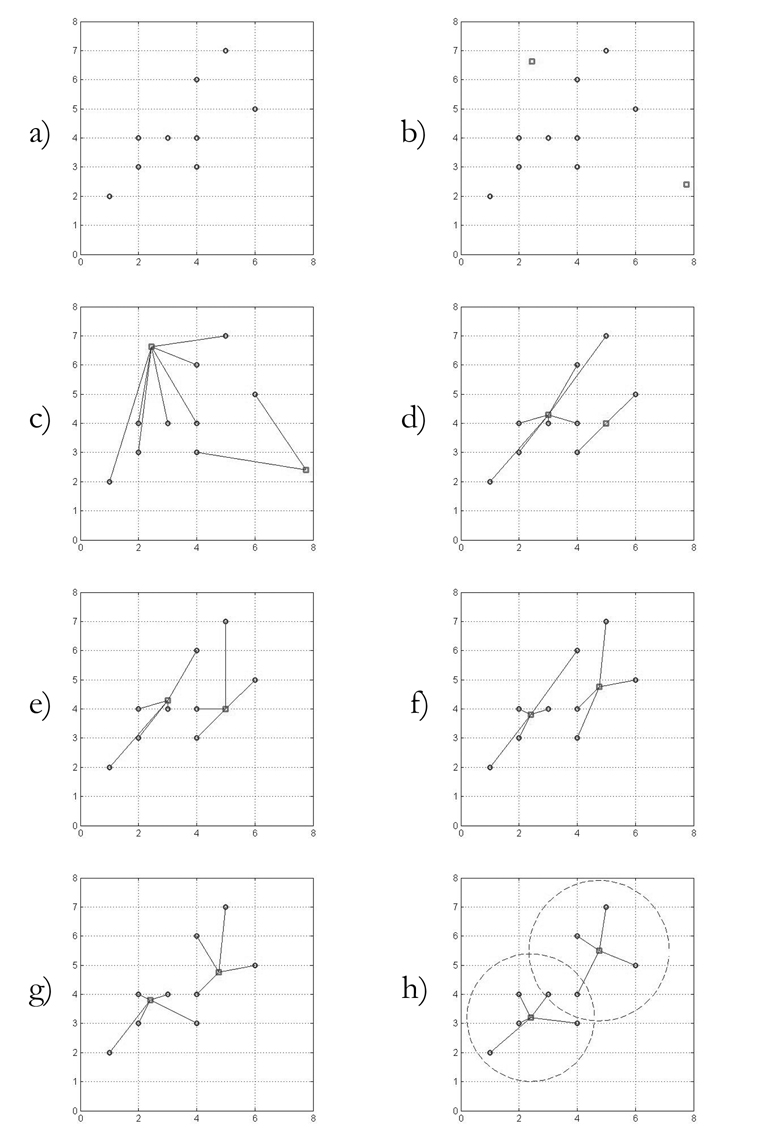
Figure 2: Presentation of the classical dynamic clustering method. a) set of $9$ data points represented by the circles which need to be partitioned into $2$ clusters - b) same as a) with the addition of the $2$ starting seeds for the clustering procedure (squares) - c) & d) $1^{st}$ iteration (see main text) - e) & f) $2^{nd}$ iteration - g) & h) $3^{rd}$ and last iteration - the circles in dashed-line in h) give an idea of the size of clusters.

We first define a set of $N$ datapoints $(x_{i},y_{i})$, with $i=1,N$. Fig. 2 (stage a) is an example with $N=9$. Our goal is to partition this dataset into a given number $N_{c}$ of clusters, with $N_{c}<N$. In the example illustrated in Fig. 2, $N_{c}=2$. The first step consists in throwing $2$ more points at random represented with square symbols (stage b)). Note that those added points can be chosen to coincide with points belonging to the initial dataset. We now link each circle to the closest square, and obtain a first partition of the dataset into $2$ clusters (stage c)). The first cluster features $2$ datapoints, while the second cluster features $7$ data points in our example. Each square is now moved to the barycenter of the associated cluster (stage d)), leaving the partition intact. As the squares change position, so do the distances between squares and circles. We link once again each circle to the closest square, which updates the partition (stage e)). Clusters now feature respectively $4$ and $5$ data points. Squares are then moved once again to the barycenters of the associated clusters (stage f)). We associate once more each circle to the closest square (stage g)), which updates the partition to a new one, the squares being moved to the barycenters of the corresponding clusters. We obtain stage h (the signification of the dashed-line circles will be given below). One can then check that any further iteration doesn’t change the partition anymore (that is, the location of the squares), so that the method converges to a fixed structure, which is the final partition of the dataset.

For any given partition, we can compute the inertia of each cluster $i_{c}$ (featuring $N_{i_{c}}$ points) by:

$$I_{i_{c}}=\frac{1}{N_{i_{c}}}\sum_{j=1}^{N_{i_{c}}}D_{j}^{2}$$ (1)

where $D_{j}$ is the distance between one point belonging to the cluster $i_{c}$ and the barycenter of that cluster. It can then be proven that the final partition we obtain minimizes the sum of inertia over all clusters. However, there can exist several local minima for the global inertia in the partition space, so that one has to run the dynamic clustering procedure several times, using different initial location of the squares in order to select the partition which corresponds to the genuine global minimum. Stage h shows the final partition we obtained starting from stage b, with $2$ dashed-line circles. Each circle is centered on the barycenter of a cluster, and its radius is taken as twice the square root of the inertia of that cluster. The role of those circles is just to illustrate the size of each cluster, and the way we quantify this size will become clearer later. The total variance in stage h is $3.5375$ (note that coordinates are dimensionless in our example).

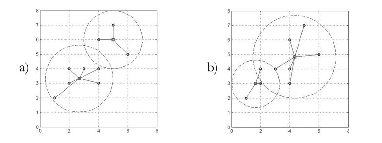
Figure 3: Final partitions for the same data set as in Fig. 1a) obtained for $2$ different starting configurations of the seed points (squares). The partition in a) corresponds to the global minimum of the sum of inertia over both clusters.

We performed this dynamic clustering process using hundreds of different initial positions for the squares, and were able to find two other local variance minima (with corresponding partitions illustrated on Fig. 3a and 3b). The final inertia of the configuration shown in Fig. 3a is $3.1111$, while the one we computed for Fig. 3b is $3.5833$. The partition which minimizes the global inertia is thus the one shown on Fig. 3a. Note however that those three minima are not very different from each other, so that all of them appear as very reasonable partitions. The similarity of the numerical values of the variances suggests that all three partitions would be barely discriminated by a human operator alone, which one generally refers to as ‘subjectivity’. Note also that the final partitions display data points that lay almost half-way between two squares, so that adding some noise on the positions of the data points (to simulate earthquake localization uncertainties) would certainly make a given final partition switch to one of the two others, and vice-versa.

3.2 The problem of anisotropy in 3D - Principal component analysis

Dynamic clustering, as described in the previous section, is an iterative procedure which minimizes the sum of variances over a given number of clusters. As presently set up, dynamical clustering suffers from the two following drawbacks:

• the user has to choose a priori the number of clusters necessary to partition our data set; the method to remove this constraint will be addressed in the next section;

• Using a criterion in terms of the minimization of the total inertia is certainly not adequate when data points have to be partitioned into anisotropic clusters, as we plan to do by associating earthquakes with faults. As an alternative, we propose a minimization criterion which takes account of the whole inertia tensor of each cluster.

The inertia tensor of a given cluster of points embedded in a $3D$ space is equivalent to the covariance matrix of their coordinates $(x,y,z)$. The covariance matrix $C$ reads :

$$C=\left(\begin{array}[]{ccc}\sigma_{x}^{2}&{\rm cov}(x,y)&{\rm cov}(x,z)\\ {\rm cov}(x,y)&\sigma_{y}^{2}&{\rm cov}(y,z)\\ {\rm cov}(x,z)&{\rm cov}(y,z)&\sigma_{z}^{2}\end{array}\right)$$ (2)

where the diagonal terms are the variances of the variables $x,y$ and $z$, while the off-diagonal terms are the covariances of the pairs of variables. Diagonalizing the covariance matrix provides a set of three eigenvalues and their associated eigenvectors. The largest eigenvalue $\lambda_{1}^{2}$ provides an information on the largest dimension of the cluster (thereafter considered as its length), and its associated eigenvector $\vec{u_{1}}$ provides the direction along which the length is striking. The second largest eigenvalue $\lambda_{2}^{2}$ (and its eigenvector $\vec{u_{2}}$) gives the same kind of information for the width of the cluster, while the smallest eigenvalue $\lambda_{3}^{2}$ (and its eigenvector $\vec{u_{3}}$) gives an information on the thickness of the cluster. If we now consider that data points cluster around a fault, eigenvalues and eigenvectors provide the dimensions and orientations of the fault plane, the third eigenvector being normal to the fault plane.

The relationship between an eigenvalue and the dimension of the fault along the associated direction depends on the specific distribution of points on the plane. In the following, we shall assume for simplicity that data points are distributed uniformly over a plane, so that the length of the fault $L$ is $\lambda_{1}\sqrt{12}$, and its width $W$ is $\lambda_{2}\sqrt{12}$. The square root of the third eigenvalue is the standard deviation of the location of events perpendicularly to the fault plane. If the fault plane really represents the fault associated with the earthquakes, the standard deviation of the location of events perpendicularly to the fault plane should be of the order of the localization uncertainty. Our idea is to partition the data points by minimizing the sum of all $\lambda_{3}^{2}$ values obtained for each cluster, so that the partition will converge to a set of clusters that tend to be as thin as possible in one direction, while being of arbitrary dimension in other directions. This procedure defines a set of fault-like objects in the most natural way possible. For each cluster, the knowledge of the third eigenvector $\vec{u_{3}}$ is then sufficient to determinate the strike and dip of the fault.

4 A new method: the 3D Optimal Anisotropic Dynamic Clustering

4.1 Definition of the 3D Optimal Anisotropic Dynamic Clustering

The general problem we have to solve is to partition a set of earthquake hypocenters into separate clusters labelled as faults. The previous section presented the general method to determine the size of a cluster as well as a new minimization criterion for anisotropic dynamic clustering. We shall now give a brief overview of a new algorithm that we propose, which also performs the automatic determination of the number of clusters to be used in the partition. This last property is particularly important in order for the fault network to be entirely deduced from the data with no a priori bias. To simplify at this stage of development (this can be refined in the future), we consider that the localization uncertainty of earthquakes is uniform in the whole catalog and equal to $\Delta$. The idea is thus that all clusters should be characterized by $\lambda_{3}<\Delta$. If not, part of the variance may be explained by something else than localization errors, i.e. another fault. The algorithm can be described as follows.

1. We first consider $N_{0}$ faults with random positions, orientations and sizes.

2. For each earthquake in the catalog, we search for the closest fault and associate the former to the latter. This provides a partition of seismic events in clusters.

3. For each cluster, we compute the position of its barycenter as well as its covariance matrix. This matrix is diagonalized, which provides its eigenvectors and eigenvalues. From those last parameters, we compute the strike, the dip, the length and the width, i.e. the characteristics of the fault which explain best the given cluster. The center of the fault is located at the barycenter of the cluster.

4. If we have $\lambda_{3}<\Delta$ for all clusters, the computation stops, as the dispersion of events around faults can be fully explained by localization errors. If not, we get back to step (2) and loop until we converge to a fixed geometry. Then, if there is at least one cluster for which $\lambda_{3}>\Delta$, we get to step (5).

5. We split the thickest cluster (the one which possesses the largest $\lambda_{3}$ value) by removing the associated fault and replacing it by at least $2$ other faults with random positions within that cluster. Obviously the cluster with the largest $\lambda_{3}$ is the one which needs most to be fitted using more faults. Note that this step increases the total number of fault $N_{0}$ used in the partition.

6. We go back to step (2).

The computation then stops when there are enough faults in the system to split the set of earthquake hypocenters in clusters that all obey the condition $\lambda_{3}<\Delta$. In addition, we remove from further analysis those clusters which contain too few events or the earthquakes which are spatially isolated.

4.2 Tests on synthetic datasets

This algorithm has been tested on synthetic sets of events. The synthetic catalog of earthquakes has been constructed as follows. We first choose the number of faults as well as their characteristics. We then put at random some data points on those planes, and add some noise to simulate the localization uncertainty characterizing the location of natural events. This set of data points is then used as an input for the new algorithm presented in the previous section. Our goal is to check if the algorithm is able to find the characteristics of the original fault network. As we want to ensure that no a priori knowledge of the dataset can contaminate the determination of the clusters, we start the algorithm with an initial number of faults equal to $N_{0}=1$.

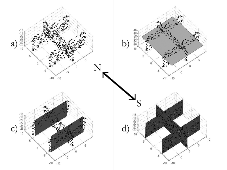
Figure 4: Step by step progression of the optimal anisotropic dynamic clustering procedure proposed in this article, which is applied to a synthetic dataset. Panel a) shows the $3D$ dataset - Panel b) shows a fit with $1$ plane - Panel c) shows the best fit with $2$ planes - Panel d) shows the best fit with $3$ planes. In this last case, we recover the correct set of planes with which the data set had been generated.

We shall begin by detailing the example shown in Fig. 4a. This dataset has been generated using two parallel planes, each of them being normal to a third one. All planes are vertical. Two planes strike $N90$ (and are located $12km$ apart) while the third one strikes $N0$. All planes are $20km$ long and $10km$ wide. Two hundred earthquakes are located randomly on each of those three planes while a random white noise in the interval $[-0.01km;+0.01km]$ is added to each coordinate of every earthquake. We set $\Delta=0.01km$ and start the 3D Optimal Anisotropic Clustering algorithm on this dataset. As we start with $N_{0}=1$, the algorithm first fits the dataset with a single plane determined from the covariance matrix of the whole catalog, giving the solution shown in Fig. 4b. Note that the best fitting plane is horizontal, and thus does not reflect at all the original geometry. Its length is $19.667$ km and its width is $16.798$ km. For that plane, we find $\lambda_{3}=5.038$ km $>\Delta$, so that a second plane is introduced in order to decrease $\lambda_{3}$. The algorithm then converges to the fit proposed in Fig. 4c. The plane $A$ strikes $N90$ and dips $S86$. Its length is $16.985$ km and its width is $9.944$ km. Its $\lambda_{3}$ value is $2.933$ km. The plane $B$ strikes $N90$ and dips $N87$. Its length and width are respectively $16.985$ km and $10.073$ km. Its $\lambda_{3}$ value is $3.043$ km. The two planes stand $11km$ apart. The cluster associated to plane $A$ being the thickest (and its thickness being larger than $\Delta$), we split its plane in two, so that there are now three planes available to fit the data. After a few iterations, the algorithm converges the structure shown in Fig. 4d. One can check that the spatial location of each plane is correct, while the azimuts and dips are determined within an error of less than $0.005$ degrees. The dimensions of the planes are determined within $3\%$. The value $\lambda_{3}$ for each plane is slightly lower than $\Delta$. The algorithm has thus found by itself that it needed three planes to fit correctly the dataset, the remaining variance being explained by the localization errors.

Using synthetic tests developed to demonstrate the power of the method, we considered several other fault geometries, with varying strikes, dips and dimensions. It is worth noting that the spatial extent of the reconstructed fault structure was found with great accuracy in each case. Our synthetic tests have been performed with a seismicity uniformly distribution on the fault planes. In the future, we plan to perform more in-depth tests with synthetic catalogs on more complex multi-scale fault networks in the presence of a possible non-uniform complex spatial organization of seismicity, so as to better mimic real catalogs. But since, as we shall see in the next section, the extents of faults inverted form natural data sets seem reasonable as well (see next section), we conjecture that our method is robust with respect to the presence of heterogeneity.

4.3 Application to the Landers aftershocks sequence

4.3.1 Implementation

As the method yields correct results on simple synthetic examples, we are encouraged to apply it to real time series, such as the aftershock sequence of the 1992 Landers earthquake in Southern California. We used the locations provided by Shearer et al (2005) and considered only the first two weeks of aftershock activity, i.e. a set of $3503$ events. We used such a limited subset of the full sequence due to limits set by the required computation time. In the future, we plan to parallelize the algorithm in order to be able to deal with much larger catalogs. The relative localization uncertainty is reported to be a few tens of meters y Shearer et al (2005), but we set $\Delta=1$ km to perform a first coarse scale inversion. Our justification for setting $\Delta=1$ km is twofold. First, the absolute localization errors are certainly larger than a few tens of meters. Second, using a value of $\Delta$ smaller than $1$ km would imply to use a much larger catalog, with many more events to sample correctly small-scale features, hence increasing the computation time prohibitively. We detail hereafter the progression of the algorithm as the number of introduced faults increases, as we did in the previous section for the synthetic case shown in Fig. 5a to 5f. As the $3D$ spatial structure of the sequence is quite complex, we show only the projection of the results on the horizontal plane.

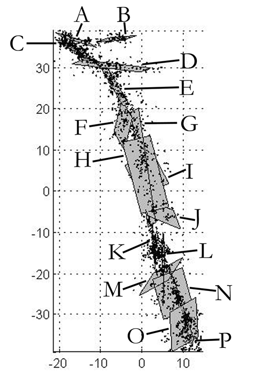
Figure 6: Fit with $16$ fault planes of the 1992 Landers, California, aftershock data set. The value $\lambda_{3}$ of each cluster is smaller than the imposed resolution threshold $\Delta=1$ km.

Stage a) shows the result of the fit with a single fault, for which we obtain $\lambda_{3}=2.9$ km. Since this value is larger than $\Delta=1$ km, we introduce a second fault, and obtain the pattern shown in stage b). The second fault is found to increase the quality of the fit mainly at the southern end of the sequence, where a large amount of events are located. The largest $\lambda_{3}$ is still about $2.9$ km. We thus introduce a third fault, with the optimal three fault structure shown in stage c). The new fault now helps to increase the quality of the fit in the northern end. Notice that this third fault is found to be horizontal, a signature of the competition between several strands as observed in the synthetic test presented in Fig. 4b. Indeed, one can observe visually that this northern region is characterized by at least three branches, which explains the optimization with an horizontal northern fault. The value $\lambda_{3}$ for this last fault is about $2.5km$, leading to the introduction of a fourth fault, whose optimal structure is shown in stage d). Now, the northern end is fitted more satisfactorily, and the largest $\lambda_{3}$ value drops to $1.8km$. The algorithm thus continues to introduce new faults, and we step directly to the pattern we obtain with $8$ faults which is shown in Fig. 5e. At this stage, the algorithm has dissected the central part of the dataset, but still does not provide a good fit to the branch at $30km$ North of the origin. As the largest value $\lambda_{3}$ is $1.4km$, the algorithm still needs more faults. Fig. 5f shows the optimal fault structure fitting the data set of aftershock hypocenters with $12$ faults. The northern part now appears to be fitted very nicely, while the southern part looks quite complex. As the largest value $\lambda_{3}$ is now $1.14km$, the algorithm needs more faults to fit the data with the threshold condition $\Delta=1$ km. We find that the largest value $\lambda_{3}$ drops below $\Delta=1$ km for $16$ faults, for which the computation stops and yields the final pattern shown in Fig. 6. When interpreting this figure, it is important to realize that some fault planes are nearly vertical, which make them barely visible in the projection shown in Fig. 6.

In order to describe the fault network, it is convenient to label the $16$ faults from $A$ to $P$, which allows us to discuss this pattern fault by fault. The parameters of the $16$ fault planes (size and orientation) are given in Table 1. These fault planes will now be classified into three different catagories, namely (i) spurious planes (which have no tectonic significance) (ii) previously known planes (that correspond to mapped faults) (iii) unknown planes (that may correspond to blind faults or to otherwise structures unmapped for whatever reason).

4.3.2 Spurious planes

An inspection of Table 1 reveals that most proposed planes dip close to the vertical. Three planes, $H$, $I$ and $N$ have rather abnormal dips, which leads us to suspect that they are spurious. Indeed, $H$ and $I$ are near normal to the plane $G$, which is located in a zone with rather diffuse seismicity in the direction normal to that plane. Introducing planes $H$ and $I$ is a convenient way to reduce the variance in that zone. It is likely that those planes have no tectonic significance, but have been found by the algorithm as the way to satisfy the criterion on $\lambda_{3}$ (we shall come back below to this argument). Plane $N$ also seems to be introduced just to decrease the variance in a zone displaying fault branching. All other $13$ fault planes out of the $16$ have dips larger than $50$ degrees, so that we have a priori no reason to remove them.

4.3.3 Previously known faults

Because the fault planes have been obtained by fitting seismicity data, none of them cross-cut the free surface. It is however interesting to compare the planes in Fig. 6 to the faults mapped at the surface in the Landers area (see Liu et al, 2003), and to underline possible correspondances. For example, plane $C$ clearly corresponds to the southern end of the Camp Rock fault. Plane $E$ corresponds to the Emerson fault. Plane $G$ is a good candidate for the Homestead Valley fault. Note that surface faulting is quite complex and diffuse in that zone. Continuing to the South, planes $K$ and $L$ seem to match respectively with the Johnson Valley and Brunt Mountain faults, while plane $P$ is the Eureka Peak fault. All those faults are known to have been activated during the Landers event. Plane $F$ is located in quite a complex faulting zone, but its azimuth fits well with both the Northern end of the Homestead Valley fault or with the Upper Johnson Valley fault. In the former case, plane $G$ would then fit with most of the Homestead Valley fault and the Maume fault. Plane $J$ is also located in a zone of complex faulting, and it is difficult to guess if it corresponds to the Southern end of the Homestead Valley fault, or to the Kickapoo fault. Note that it may also feature events from both faults.

4.3.4 Unknown faults

This last set contains planes $A$, $B$, $D$, $M$ and $O$. Planes $A$, $B$ and $D$ obviously fit blind faults, that one can guess, for instance, in Fig. 7 which plots the full set of events in Shearer et al (2005)’s catalog in the same area. In the Southern end, plane $M$ may fit with the Pinto Mountain fault, while $O$ would be a genuine blind fault.

5 Discussion and Conclusion

We have introduced a new powerful method, the 3D Optimal Anisotropic Dynamic Clustering, that allows us to partition a $3D$ set of earthquakes hypocenters into distinct anisotropic clusters which can be interpreted as fault planes. The method was first applied to a variety of synthetic data sets, which confirmed its ability to recover correctly with high accuracy the existence of present faults. We then applied the 3D Optimal Anisotropic Dynamic Clustering to the sequence of aftershocks following the 1992 Landers event in California. In this later case, we were able to recognize the faults that were already known by surface mapping. In addition, the 3D Optimal Anisotropic Dynamic Clustering method allowed us to identify some additional blind faults. These faults appear to make sense when looking at the long-term epicenter maps or $3D$ plots of seismicity. The advantage of our method is that it finds automatically the characteristics of the fault planes as well as the hypocenters that belong to each of them, without any need for the operator to pick them manually. The method provides the orientation of the faults, as well as the size of their active part during the earthquake sequence used to identify them.

The main drawback of this method is that it can propose fault planes that are likely spurious (error of type II), as they lack any tectonic meaningful interpretation. This problem appears in the presence of diffuse seismicity, for which the 3D Optimal Anisotropic Dynamic Clustering method forces the introduction of fault planes in the diffuse zone in order to reduce the global variance of the distances from earthquakes to the proposed fault planes. In the case of the Landers aftershock sequence, we were able to sort them out from their anomalous dip parameters, compared with all known fault planes in the Landers area which are nearly vertical, as also confirmed by focal mechanisms. This post-processing step will become much more subjective when trying to sort out spurious planes in more complex tectonic settings. We thus believe that our procedure should use additional information available in earthquakes catalogs than just the 3D hypocenter locations. For example, focal mechanism characteristics are now determined for a large number of events, so that the inertia of a cluster should use not only the position of a given event in the cluster, but also a criterion of compatibility of the focal mechanism of this event with the orientation of the best fitting plane of that same cluster. The idea is to make the algorithm converge to a set of anisotropic clusters over which the distribution of focal mechanisms is approximately uniform. This extension of the method will be developed and tested elsewhere.

In the same vein, we propose another future extension of the 3D Optimal Anisotropic Dynamic Clustering consisting of using the information on waveforms contained in the Southern California earthquakes catalog of Shearer et al (2005). The method used to build this catalog consists in grouping events according to the similarity of their waveforms. This first step thus yields a proto-clustering of events. Time-delays of wave arrival times for events belonging to the same proto-cluster yield relative locations of those grouped events. Events belonging to the same proto-cluster display similar waveforms and are thought to be characterized by similar rupture mechanisms, thus may betray successive ruptures on the same fault. Shearer et al (2005) used this idea and performed principal component analyses on each proto-cluster of the Northridge, California, aftershocks sequence. This idea is similar to ours, but nothing proves that a single proto-cluster samples only one fault segment. For example, when looking at the seismicity in the Imperial fault area, Shearer (2002) has been able to identify some very fine-scale features in earthquakes clouds that otherwise looked very fuzzy. In this last example, a proto-cluster of events was found to be clearly composed of two parallel lineaments, with a $500m$ offset between them. However, the operator still has to use a ruler and a protractor to compute the dimension and orientation of each lineament, and his eyes to count them. Using a method such as ours on that specific proto-cluster would naturally partition it into two (sub)clusters, and provide their associated dimensions and orientations. Thus, a natural future application of our method would be to apply it on each of the clusters resulting from Shearer et al (2005)’s proto-partition. The advantage is that the number of events in each cluster is small, so that the algorithm will converge very quickly, and that events will be already pre-sorted according to the similarity of their rupture mechanism. The fact that all events within proto-clusters are located with an accuracy of the order of few tens of meters should allow one to provide a very detailed fit of the $3D$ spatial structure of the catalog.

We would also like to stress that the 3D Optimal Anisotropic Dynamic Clustering method provides a natural tool for understanding the multiscale structure of fault zones. In a recent paper, Liu et al (2003) showed that the spatial dispersion of aftershocks epicenters normal to the direction of Landers main rupture could not be explained by localization errors alone, betraying the complex mechanical behaviour of this fault zone. In the examples presented in this paper, we considered that the resolution parameter $\Delta$ controlling the number of faults necessary to explain the seismic data could be mapped in a natural way on the spatial localization uncertainty of the spatial location of the events. While this is a natural choice, more generally, $\Delta$ can take any arbitrary value assigned by the user and, in such a case, it must be interpreted as the spatial resolution at which the user wants to approximate the anisotropic fault structure defined by the catalog of events. For example, if we consider the choice $\Delta=10km$, the output is the same as the one presented on Fig. 5a, as only one fault is necessary to fit the data at this coarse resolution. As we make $\Delta$ decrease, the number of necessary faults increases as we have seen. Fig. 7 shows that the number of fault planes necessary to fit the Landers’ data varies with $\Delta$ as

$$N(\Delta)\simeq\Delta^{-\mu}~{},\quad{\rm with}\quad\mu=2~{},$$ (3)

over a limited range. For very large $\Delta$’s, it is obvious that just one fault is necessary. This powerlaw behaviour is of course reminiscent of a scale-invariant geometry, but we still have to clarify a few points before any further serious conclusion. The first one is a theoretical one: usual methods used to compute the fractal dimension of a given object consider scale-dependent approximations of that object with isotropic balls (for example, box-counting uses isotropic balls with the $L_{1}$ norm, while the correlation method uses isotropic balls with the $L_{2}$ norm). In the present case, we approximate our dataset by highly anisotropic “balls,” which in addition do not have the same size. It thus seems inappropriate to interpret $\mu$ as a genuine fractal dimension. The second is a pragmatic one: for a given scale-invariant distribution of points, the measured fractal dimension depends on its cardinal number. The reason is that, the largest is the cardinal, the better the distribution is sampled, and the better is its statistical characterization. If the cardinal is low, the multi-scale structure of the distribution is not properly sampled and the measured fractal dimension is biased. As we still do not know the effect of the bias that may affect the determination of the exponent $\mu$, much more work is needed in that direction.

Considering earthquake forecasting and seismic hazard assessment, the knowledge of the fault network architecture in the vicinity of large events will also help to test different competing hypothesis on stress transfer mechanism. Until now, two strategies have been used in order to check for the consistency between the geometry of the main shock rupture and the spatial location of aftershocks. The first one considers that all rupture planes of aftershocks are parallel to the main rupture. The second one postulates that the rupture planes are optimally oriented. None of those hypotheses turn out to be true (see Steacy et al (2005)). Therefore, we think that imaging accurately the $3D$ structure of a fault network constitutes one of the most important steps in order to decipher static or dynamic earthquake triggering. The 3D Optimal Anisotropic Dynamic Clustering provides a first significant step in this direction.

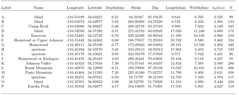
Figure 1: Table of correspondances between fitting planes of the Landers, California, sequence and faults in the same area. Each fitting plane is qualified by the label given on Fig. 6. The name of the corresponding fault is given in the second column. Spurious indicates that the plane certainly has no tectonic significance, while blind signifies that the fault doesn’t intersect the free surface. Each plane is characterized by the latitude, longitude and depth of its center, as well as its strike, deep and dimensions in $km$. The $2$ last columns feature the $\lambda_{3}$ value of the corresponding cluster and the total number of events that belong to that cluster.

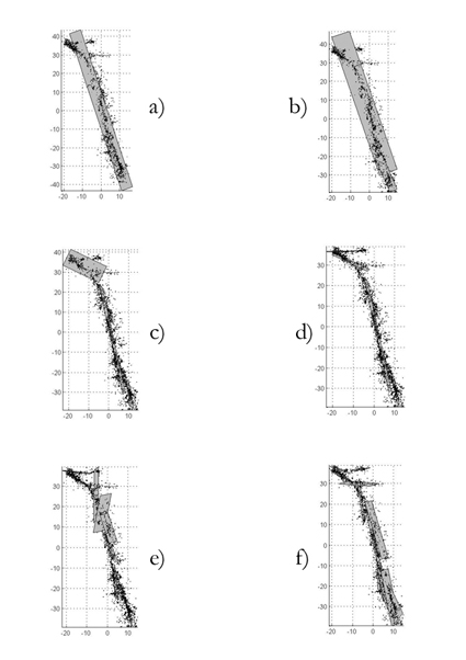
Figure 5: Progression of our method of dynamic clustering when applied to a subset of the 1992 Landers, California, aftershocks sequence. a) fit of the sequence with $1$ plane - b) fit with $2$ fault planes - c) fit with $3$ fault planes - d) fit with $4$ fault planes - e) fit with $8$ fault planes - f) fit with $12$ fault planes.

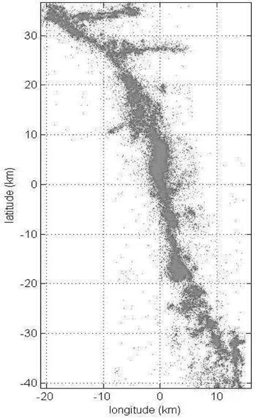
Figure 7: Epicentral view of the full catalog available for the Landers earthquake.

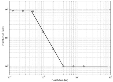
Figure 8: Number of fault planes necessary to fit the set of aftershocks of the Landers earthquake, as a function of the resolution $\Delta$. Note the finite range of scales over which the power law behavior $N(\Delta)\simeq\Delta^{-2}$ is valid.

References

- [1] Bhattacharya, P., H. Liu, A. Rosenfeld and S. Thompson (2000), Hough transform detection of lines in 3D space, Pattern Recognition Letters, 47, 65-73.
- [2] Béthoux, N., G. Ouillon and M. Nicolas (1998), The instrumental seismicity of the Western Alps: spatio-temporal patterns analysed with the wavelet transform, Geophys. J. Int., 135, 177-194.
- [3] Darrozes, J., P. Gaillot and P. Courjault-Radé (1998), propagation of a sequence of aftershocks combining anisotropic wavelet transform and GIS, Phys. Chem. Earth, 23, 303-308.
- [4] Duda, R.O. and P.E. Hart (1972), Use of the Hough transformation to detect lines and curves in pictures, Comm. ACM, 15, 11-15.
- [5] Faulkner, D. R., A.C. Lewis and E.H. Rutter (2003), On the internal structure and mechanics of large strike-slip fault zones: field observations of the Carboneras fault in southeastern Spain, Tectonophysics, 367, 235-251.
- [6] Gaillot P., J. Darrozes, M. De Saint Blanquat and G. Ouillon (1997), The normalised optimised anisotropic wavelet coefficient (NOAWC) method: an image processing tool for multi-scale analysis of rock fabric, Geophys. Res. Lett., 24, 14, 1819-1822.
- [7] Gaillot, P., J. Darrozes and J.L. Bouchez (1999), Wavelet transforms: the future of rock shape fabric analysis?, J. Struct. Geol., 21, 1615-1621.
- [8] Gaillot, P., J. Darrozes, P. Courjault-Radé and D. Amorese (2002), Structural analysis of hypocentral distribution of an earthquake sequence using anisotropic wavelets: method and application, J. Geophys. Res., 107 (B10), 2218, doi:10.1029/2001JB0000212.
- [9] Grégoire, V., J. Darrozes, P. Gaillot, P. Launeau and A. Nédélec (1998), Magnetite grain shape fabric and distribution anisotropy versus rock magnetic fabric: a 3D-case study, J. Struct. Geol., 20, 937-944
- [10] Helmstetter, A., G. Ouillon and D. Sornette (2003), Are aftershocks of large Californian earthquakes diffusing?, J. Geophys. Res., 108, 2483, 10.1029/2003JB002503.
- [11] Liu, J., K. Sieh and E. Hauksson (2003), A Structural Interpretation of the Aftershock ”Cloud” of the Landers Earthquake, Bull. Seism. Soc. Am. 93, 1333-1344.
- [12] Mac Queen, J. (1967), Some methods for classification and analysis of multivariate observations, pp. 281-297 in: L. M. Le Cam and J. Neyman [eds.] Proceedings of the fifth Berkeley symposium on mathematical statistics and probability, Vol. 1. University of California Press, Berkeley. xvii + 666 p.
- [13] Ouillon, G. (1995), Application de l analyse multifractale et de la transformée en ondelettes anisotropes à la caractérisation géométrique multiéchelle des réseaux de failles et de fractures, Documents du BRGM, 246.
- [14] Ouillon G. , C. Castaing and D. Sornette (1996), Hierarchical Geometry of Faulting, J. Geophys. Res., 101 (B3), 5477-5487.
- [15] Ouillon, G. and D. Sornette (1996), Unbiased Multifractal Analysis of Fault Patterns, Geophys. Res. Lett., 23, 23, 3409-3412.
- [16] Passchier, C.W. and R.A.J. Trouw (2005), Microtectonics, Springer Verlag.
- [17] Plesch, A. and Shaw, J. H. (2002), SCEC 3D Community Fault Model for Southern California, Eos Trans. AGU, Fall Meet. Suppl., 83, Abstract S21A-0966. (http://structure.harvard.edu/cfm includes Broderick, Kamerling and Sorlien maps).
- [18] Pollard, D. D. and R.C. Fletcher (2005), Fundamentals of Structural Geology, Cambridge University Press.
- [19] Sarti, A. and S. Tubaro (2002), Detection and characterization of planar fractures using a 3D Hough transform, Signal Processing, 82, 1269, doi:10.1016/S0165-1684(02)00249-9.
- [20] Scholz, C. (2002), The Mechanics of Earthquakes and Faulting, Cambridge University Press.
- [21] Shearer, P.M. (2002), Parallel fault strands at 9-km depth resolved on the Imperial Fault, Southern California, Geophys. Res. Lett., 29, 1674, doi:10.1029/2002GL015302.
- [22] Shearer, P.M., J.L. Hardebeck, L. Astiz and K.B. Richards-Dinger (2003), Analysis of similar event clusters in aftershocks of the 1994 Northridge, California, earthquake, J. Geophys. Res., 108 (B1), 2035, doi:10.1029/2001JB000685.
- [23] Shearer, P., E. Hauksson and G. Lin (2005), Southern california hypocenter relocation with waveform cross-correlation, part 2: Results using source-specific station terms and cluster analysis, Bulletin of the Seismological Society of America, 95, 904-915.
- [24] Sornette, D. (1991) Self-organized criticality in plate tectonics, in the proceedings of the NATO ASI “Spontaneous formation of space-time structures and criticality,” Geilo, Norway 2-12 april 1991, edited by T. Riste and D. Sherrington, Dordrecht, Boston, Kluwer Academic Press, volume 349, p.57-106.
- [25] Sornette, D., Ph. Davy and A. Sornette (1990) Structuration of the lithosphere in plate tectonics as a self-organized critical phenomenon, J. Geophys. Res. 95, 17353-17361.
- [26] Steacy, S., S.S. Nalbant, J. McCloskey, C. Nostro, O. Scotti and D. Baumont (2005), Onto what planes should Coulomb stress perturbations be resolved?, J. Geophys. Res., 110 (B05S15), doi:10.1029/2004JB003356.
- [27] Wesson, R. L., W. H. Bakun and D.M. Perkins (2003), Association of earthquakes and faults in the San Francisco Bay area using Bayesian inference, Bulletin of the Seismological Society of America, 93, 1306-1332.