Theoretical investigation of finite size effects at DNA melting

Abstract

We investigated how the finiteness of the length of the sequence affects the phase transition that takes place at DNA melting temperature. For this purpose, we modified the Transfer Integral method to adapt it to the calculation of both extensive (partition function, entropy, specific heat, etc) and non-extensive (order parameter and correlation length) thermodynamic quantities of finite sequences with open boundary conditions, and applied the modified procedure to two different dynamical models. We showed that rounding of the transition clearly takes place when the length of the sequence is decreased. We also performed a finite-size scaling analysis of the two models and showed that the singular part of the free energy can indeed be expressed in terms of an homogeneous function. However, both the correlation length $\xi$ and the average separation between paired bases $\left<y\right>$ diverge at the melting transition, so that it is no longer clear to which of these two quantities the length $L$ of the system should be compared. Moreover, Josephson’s identity is satisfied for none of the investigated models, so that the derivation of the characteristic exponents which appear, for example, in the expression of the specific heat, requires some care.

^(♯)email : Marc.JOYEUX@ujf-grenoble.fr

I Introduction

Real systems manifesting critical behavior have necessarily finite volume. However it is well-known that the finiteness of the system size lets the critical singularities disappear and smears out the phase transition (see for example [1-5]). The obvious argument which may reconcile these two aspects is that, as the finite size of the system is increased and passes through a critical value which characterizes the border of the thermodynamical domain, the thermodynamical limit is approximately reached and consequently the critical singularities manifest themselves. Thus it is crucial to thoroughly understand the evolution of singularities with respect to the system size and estimate the critical size above which the thermodynamical limit is attained.

An efficient tool to analyze the volume dependence of a critical phenomenon is the finite size scaling theory. Besides providing information on the rounding of critical singularities and the shift in the critical point, this theory is also an alternative way to determine critical exponents characterizing the phase transition.

Finite size scaling theory was developed by Fisher and Barber in the early seventies 6 (6). During the last thirty years it has been applied to various systems exhibiting both first and second order phase transitions. Among hundreds of subjects we can mention the study of finite size effects at first order transitions by gaussian approximation [7-8], the Gibbs ensemble 9 (9), five dimensional Ising model [10-11], percolation models [12-13], stochastic sandpiles 14 (14), six-dimensional Ising system 15 (15), Baxter-Wu model 16 (16), two dimensional anisotropic Heisenberg model 17 (17)…

In nature, the majority of phase transitions are sharp and discontinuous first order transitions. Experimental UV absorption spectra of diluted DNA solutions reveal that the DNA melting transition belongs to this class. A widely used dynamical non-linear DNA model was proposed twenty years ago by Peyrard and Bishop 18 (18). This model involving harmonic interaction terms between successive base pairs was later improved by the contribution of Dauxois 19 (19) and the new model (DPB model) yields a sharp transition. We recently proposed an alternative DNA model (JB model) which respects the finiteness of the stacking energy, and showed that this model also exhibits a sharp first order phase transition 20 (20). Then in 21 (21) we showed that for both models the generalized homogeneity assumption is not respected so that Josephson’s identity (also known as the hyperscaling relation) is not valid. We tentatively explained this fact by the divergence of the order parameter at the critical point.

The goal of this article is to investigate the sequence length dependence of the DNA melting transition. This is an important point since experiments dealing with DNA molecules are carried out with various sequence lengths. To this end we employ a modified transfer integral method adapted to finite chains with open boundary conditions. The two hamiltonian DNA models to be studied, i.e. the DPB and the JB models, are briefly described in Sec. II. Section III deals with the transfer matrix theory for finite linear chains and Sec. IV is devoted to the finite size scaling analysis which leads to a better understanding of finite size effects.

II Non-linear Hamiltonian models for DNA

The Hamiltonians of the two DNA models whose critical behaviour is studied in this article are of the form

$$H=\sum_{n=1}^{N}\left\{\frac{p_{n}^{2}}{2m}+V_{M}(y_{n})+W(y_{n},y_{n-1})\right\}$$ (1)

where $y_{n}$ is the transverse stretching of the hydrogen bond between the nth pair of bases, while the one-particle Morse potential term

$$V_{M}(y_{n})=D\left(1-e^{-ay_{n}}\right)^{2}$$ (2)

models the binding energy of the same hydrogen bond. The choice of the nearest-neighbor interaction potential $W(y_{n},y_{n-1})$ is crucial since the type of the transition, which is a collective effect, depends primarily on its form. The DPB model 19 (19) assumes that the stacking energy is of the form

$$W(y_{n},y_{n-1})=\frac{K}{2}(y_{n}-y_{n-1})^{2}\left[1+\rho e^{-\alpha(y_{n}+y_{n-1})}\right]\hskip 1.42262pt.$$ (3)

This non-linear stacking interaction has the particularity of having a coupling constant which drops from $K(1+\rho)$ to $K$ as the critical point is approached. This decreases the rigidity of the DNA chain close to the dissociation and yields a sharp, first-order transition.

This interaction potential still has the inconvenience that the stacking energy diverges when two paired bases separate. Taking into account the finiteness of the interaction between adjacent bases, we proposed a potential of the form 20 (20)

$$W(y_{n},y_{n-1})=\frac{\Delta H}{2}\left[1-e^{-b(y_{n}-y_{n-1})^{2}}\right]+K_{b}(y_{n}-y_{n-1})^{2}$$ (4)

which, contrary to the model (3), depends only on the distance between base pairs. The small harmonic term, whose constant $K_{b}$ is 2000 times smaller than the parameter $K$ of the DPB model, was introduced in order to take into account the stiffness of the phosphate-sugar backbone.

Numerical values of the parameters are those of Refs. [19,20], that is $D=0.03\hskip 1.42262pteV$, $a=4.5\hskip 1.42262pt\mathrm{\r{A}}^{-1}$, $\alpha=0.35\hskip 1.42262pt\mathrm{\r{A}}^{-1}$, $K=0.06\hskip 1.42262pteV\hskip 1.42262pt\mathrm{\r{A}}^{-2}$, $\rho=1$ for the DPB model, and $D=0.04\hskip 1.42262pteV$, $a=4.45\hskip 1.42262pt\mathrm{\r{A}}^{-1}$, $\Delta H=0.44\hskip 1.42262pteV$, $K_{b}=10^{-5}\hskip 1.42262pteV\hskip 1.42262pt\mathrm{\r{A}}^{-2}$ and $b=0.10\hskip 1.42262pt\mathrm{\r{A}}^{-2}$ for the JB model.

III Transfer integral method for finite chains with open boundary conditions

III.1 The partition function and extensive thermodynamic quantitites

Let us define the Transfer Integral (TI) kernel according to

$$K(y_{n},y_{n-1})=exp\left[-\beta\left\{V_{M}(y_{n})/2+V_{M}(y_{n-1})/2+W(y_{n},y_{n-1})\right\}\right]$$ (5)

where $\beta=(k_{B}T)^{-1}$ is the inverse temperature. In the following analysis we deal only with sequences having open boundary conditions. Then the partition function of the system can be expressed as

$$Z=\int\,dy_{1}\,dy_{2}\cdot\cdot\cdot dy_{N}e^{-\beta V_{M}(y_{1})/2}K\left(y_{2},y_{1}\right)K\left(y_{3},y_{2}\right)\cdot\cdot\cdot K\left(y_{N},y_{N-1}\right)e^{-\beta V_{M}(y_{N})/2}.$$ (6)

The TI method consists in expanding the kernel of Eq. (5) in an orthonormal basis

$$K\left(y_{n},y_{n-1}\right)=\sum_{i}\lambda_{i}\Phi_{i}(y_{n})\Phi_{i}(y_{n-1})$$ (7)

where the $\{\Phi_{i}\}$ and $\{\lambda_{i}\}$ are the eigenvalues and eigenvectors of the integral operator and satisfy

$$\int\,dx\hskip 2.84526ptK(x,y)\hskip 1.42262pt\Phi_{i}(x)=\lambda_{i}\Phi_{i}(y)\hskip 1.42262pt.$$ (8)

This integral equation was solved by diagonalizing the symmetric TI operator $K(x,y)$ on a regularly spaced grid defined between $y_{min}=-200/a$ and $y_{max}=4000/a$ with $1/a$ intervals. Numerical integrations were performed on the same grid.

In this study we extended the transfer matrix approach for open chains developed in 22 (22) to adapt it to the calculation of the order parameter $\left<y\right>$ and the correlation length $\xi$. Let us first consider extensive thermodynamic quantities. By introducing

$$a_{i}=\int\,dye^{-\beta V_{M}(y)/2}\Phi_{i}(y)$$ (9)

and by substituting the kernel expansion of Eq. (7) into Eq. (6), we get

$$Z=\sum_{i}a_{i}^{2}\lambda_{i}^{N-1}.$$ (10)

Determination of the partition function then allows the computation of extensive quantities of the system such as the free energy, the entropy and the specific heat :

$$\begin{split}F&=-k_{B}T\ln(Z)\\ S&=-\frac{\partial F}{\partial T}\\ C_{V}&=-T\frac{\partial^{2}F}{\partial T^{2}}\hskip 2.84526pt.\end{split}$$ (11)

In the thermodynamical limit $N\rightarrow\infty$ the major contribution to the partition function arises from the largest eigenvalue $\lambda_{1}$ and in this limit it is reasonable to drop the eigenvalues with $i\geq 2$. Neverthless, we will consider large DNA molecules as well as small ones. Consequently as many eigenvalues as possible must be taken into account in numerical computations. From the practical point of view, it was found that considering the first 400 eigenvalues is enough to insure numerical convergence of the results presented below.

III.2 The order parameter and the correlation length

The order parameter of DNA melting transition is the mean separation of the bases averaged over the sites of the sequence :

$$\left<y\right>=\frac{1}{N}\sum_{n=1}^{N}\left<y_{n}\right>.$$ (12)

In order to reduce $\left<y_{n}\right>$ to a form depending only on the eigenvalues and eigenvectors of the TI operator, we first write it as

$$\left<y_{n}\right>=\frac{1}{Z}\int\,dy_{1}\,dy_{2}\cdot\cdot\cdot dy_{N}\hskip 1.42262pty_{n}\hskip 1.42262pte^{-\beta V_{M}(y_{1})/2}K\left(y_{2},y_{1}\right)K\left(y_{3},y_{2}\right)\cdot\cdot\cdot K\left(y_{N},y_{N-1}\right)e^{-\beta V_{M}(y_{N})/2}.$$ (13)

Substituting Eq. (7) into Eq. (13) and defining

$$\begin{split}b_{i}&=\int\,dye^{-\beta V_{M}(y)/2}\Phi_{i}(y)\hskip 1.42262pty\hskip 1.42262pt\\ Y_{ij}^{(1)}&=\int\,dy\Phi_{i}(y)\hskip 1.42262pty\hskip 1.42262pt\Phi_{j}(y)\hskip 1.42262pt,\end{split}$$ (14)

we obtain

$$\left<y_{1}\right>=\left<y_{N}\right>=\frac{1}{Z}\sum_{i}a_{i}b_{i}\lambda_{i}^{N-1}$$ (15)

and

$$\left<y_{n}\right>=\frac{1}{Z}\sum_{i,j}a_{i}a_{j}Y_{ij}^{(1)}\lambda_{i}^{n-1}\lambda_{j}^{N-n}$$ (16)

for $n\neq 1,N$. By evaluating the geometric summation that appears in Eq. (12) when replacing the $\left<y_{n}\right>$ by their expressions in Eqs. (15)-(16), we finally get

$$\left<y\right>=\frac{2}{ZN}\sum_{i}a_{i}b_{i}\lambda_{i}^{N-1}+\frac{1}{Z\hskip 1.42262ptN}\sum_{i,j}a_{i}a_{j}Y_{ij}^{(1)}\lambda_{i}^{-1}\lambda_{j}^{N}\frac{r_{ij}^{2}-r_{ij}^{N}}{1-r_{ij}}$$ (17)

with $r_{ij}=\lambda_{i}/\lambda_{j}$. The computation of the correlation length $\xi$ proceeds along similar lines although it is more elaborate. A sketch of the derivation and the analytical result can be found in Appendix A.

IV Finite-size effects near the critical point

IV.1 Rounding of the melting transition of DNA

It is well known that a finite-size system does not exhibit any phase transition. At the critical point its free energy is analytic and consequently all thermodynamical quantities are regular. Let $L$ be the size of a system having a critical behaviour in the thermodynamical limit $L\rightarrow\infty$. For this system finite-size effects manifest themselves as $e^{-L/\xi}$, where $\xi$ is the correlation length, by rounding the critical point singularity. In other words they become important over a region for which $\xi\sim L$. A simple example of this rounding phenomena concerning the Ising model can be found in 8 (8). For an infinite-size Ising system, as the magnetic field $H$ varies, the order parameter jumps discontinuously from $-M_{cr}$ to $+M_{cr}$ at the critical point $H=0$. On the other hand if the system’s size is finite, this transition occurs on a finite region of order $\Delta H\simeq k_{B}T/(M_{cr}L^{d})$ with a large but finite slope $\sim M_{L}^{2}L^{d}/(k_{B}T)$ where $M_{L}$ is the most probable value of the magnetization in the finite system.

For the two DNA models sketched in Sect. 2, the size $L$ of the system is equal to the number $N$ of base pairs in the sequence times the distance between two successive base pairs. This latter quantity playing no role in the dynamics of the investigated models, we will henceforth use indistinctly $N$ or $L$ to refer to the size of the sequence.

Given a sequence of length $N$, the first task consists in determining its critical temperature, which we denote by $T_{c}(N)$. Among the several methods listed for example in anan (25), we found it rather simple and convenient to search for the maximum of the specific heat $C_{V}$, which is more pronounced than that of the correlation length $\xi$, thus allowing for a more accurate localization of the temperature. Two observations confirm a posteriori that the critical temperatures thus obtained are correct. First, the shift in critical temperature is found to vary as a power of $N$, as predicted by finite-size scaling theory (see below). The top plot of Fig. 1 shows for example that $T_{c}-T_{c}(N)$, where $T_{c}$ stands for $T_{c}(\infty)$, varies as $N^{-1.00}$ and $N^{-1.05}$ for the DPB and JB models, respectively. Note that this scaling is also in excellent agreement with the semi-empirical formula used by experimentalists to calculate the melting temperature of finite sequences. Moreover, as will be seen later (Figs. 3 and 4) the curves for the temperature evolution of $C_{V}$, $\xi$, $\left<y\right>$, etc… for sequences with different lengths $N$ all coincide sufficiently far from the critical temperature when plotted as a function of the reduced temperature

$$t(N)=\frac{T-T_{c}(N)}{T_{c}(N)}\hskip 1.42262pt.$$

In order to illustrate finite-size effects acting on DNA melting, we first computed the entropy per base, $s=S/N$, for an infinite chain and a short DNA sequence for both the DPB and the JB models. Results are shown in Fig. 2. At the thermodynamic limit, the entropy $s$ is clearly discontinuous at the critical temperature, as is expected for first order phase transitions. In contrast, smooth curves are observed over the whole temperature range for the sequence with $N=100$. We next computed the specific heat per base, $c_{V}=C_{V}/N$, for increasing sequence length and temperature. The top and bottom plots of Fig. 3 show the temperature evolution of $c_{V}$ for seven values of $N$ ranging from 100 to infinity for the DPB and JB models, respectively. It is seen in this figure that rounding manifests itself through a decrease in the maximum of $c_{V}$ as $N$ decreases, but also through the fact that the sharp rise of $c_{V}$ takes place further and further from the critical temperature, that is, at increasingly larger values of $|t(N)|$. This is particularly clear for the DPB model, which at the thermodynamic limit undergoes a very sharp transition, i.e. a transition that is noticeable only at very small values of $|t|=|t(\infty)|$ 21 (21). Quite interestingly, examination of Fig. 3 also indicates that the two models consequently give very comparable results up to $N\simeq 1000$, while the narrower nature of the phase transition for the DPB model becomes apparent for longer sequences.

At this point, it should be emphasized that boundary effects may become important when the size of the system is small. In order to check whether such boundary effects play a role in the results presented above, we repeated these computations with periodic boundary conditions instead of open ones and found that this alters only very little the results for $s$ and $c_{V}$ down to $N=100$. Conclusion is therefore that boundary effects play only a marginal role down to this size.

Finally, we computed, for the JB model, the temperature evolution of the correlation length $\xi$ (Eq. (27)) and the order parameter $\left<y\right>$ (Eq. (17)) for increasing values of $N$. As the critical temperature is approached, the correlation length $\xi$ of a finite-size system is expected to increase according to the power law $\xi\propto t^{\nu}(N)$ till it reaches the system’s dimension $L$ and freezes. This behaviour can be checked in the middle plot of Fig. 1, which shows the evolution of the maximum of the correlation length (in units of the separation between successive base pairs) as a function of $N$ : the maximum of $\xi$ is indeed of the same order of magnitude as $N$ and the curve scales as $N^{0.97}$. An exception however occurs for the last three points with $N\geq 3000$ : we will come back later to this point. The bottom plot of Fig. 4 additionally shows the temperature evolution of $\xi$ for seven values of $N$ ranging from 100 to infinity. One observes just the same rounding effects as for the specific heat in Fig. 3. This is again the case for the temperature evolution of the order parameter $\left<y\right>$, which is drawn in the top plot of Fig. 4. This latter plot however displays a remarkable feature, in the sense that all the curves converge to the same limit at $T_{c}(N)$. To understand why this is the case, it must be realized that $\left<y\right>$, the average separation between paired bases, is the only quantity which diverges at the critical temperature whatever the size $N$ of the sequence, while, for example, $c_{V}$ and $\xi$ diverge for infinitely long chains but remain finite for finite chains. The limit towards which all curves converge in the top plot of Fig. 4 is thus just the approximation of infinity imposed by the numerical procedure (size of the grid, etc…).

IV.2 Finite-size scaling analysis

The basic idea of finite-size scaling is that the correlation length $\xi$ is the only length that matters close to the critical temperature and that one just needs to compare the linear dimension $L$ of the system to $\xi$ : rounding and shifting indeed set in as soon as $L/\xi\sim 1$ . Since, by definition of the critical exponent $\nu$, $\xi$ grows as $t^{-\nu}$, one has $(L/\xi)\propto{(tL^{1/\nu})}^{\nu}$ as $L\to\infty$ or, $L$ being proportional to the number $N$ of paired bases, $(L/\xi)\propto{(tN^{1/\nu})}^{\nu}$. In the absence of external field, it is therefore natural to write the singular part of the free energy of the finite-size system in the form

$$f_{sing}=N^{-d}\hskip 1.42262ptY(tN^{1/\nu})\hskip 1.42262pt.$$ (18)

where $Y$ is some homogeneous function. Differentiating Eq. (18) twice with respect to $t$, one obtains that $c_{V}$ is equal to

$$c_{V}=N^{\rho}G(tN^{\sigma})\hskip 1.42262pt,$$ (19)

where

$$\begin{split}\rho&=\frac{2}{\nu}-d\\ \sigma&=\frac{1}{\nu}\end{split}$$ (20)

and $G$ is an homogeneous function which is proportional to the second derivative of $Y$. By using Josephson’s identity, $2-\alpha=\nu d$, where $\alpha$ is the critical exponent for $c_{V}$ ($c_{V}\propto t^{-\alpha})$, coefficients $\rho$ and $\sigma$ can be recast in the form

$$\begin{split}\rho&=\frac{\alpha}{\nu}\\ \sigma&=\frac{1}{\nu}\end{split}$$ (21)

Conversely, if there occur several lengths that diverge at the critical point, as is the case for DNA melting, then it is no longer so clear to which of these lengths $L$ should be compared. In order to tackle this more complex case, Binder et al 24 (24) derived a method which is based on the use of an irrelevant variable $u$ and an expression of the form

$$f_{sing}=N^{-d}F(tN^{y_{t}},uN^{y_{u}})$$ (22)

After several approximations and a little bit of algebra, these authors obtain $c_{V}$ in the form of Eq. (19) with, however,

$$\begin{split}\rho&=\frac{2d}{2\beta+\gamma}-d\\ \sigma&=\frac{2d}{2\beta+\gamma}\hskip 1.42262pt.\end{split}$$ (23)

Finally, the lengths that diverge at DNA melting are $\xi$ and $\left<y\right>$, the average separation between paired bases. One might wonder whether $L$ should not be compared to $\left<y\right>$ instead of $\xi$. In order to check this hypothesis, let us denote by $\lambda$ the characteristic exponent for $\left<y\right>$ ($\left<y\right>\propto t^{\lambda}$). Remember that if the external field is proportional to $y$ then $\left<y\right>$ is the order parameter $m$, so that $\lambda$ is equal to $\beta$, the critical exponent for $m$ ($m\propto t^{\beta}$). Let us next express the singular part of the free energy in the form

$$f_{sing}=N^{-d}F\left(tN^{-1/\lambda}\right)\hskip 1.42262pt.$$ (24)

Differentiating Eq. (24) twice with respect to $t$, one again obtains $c_{V}$ in the form of Eq. (19) with, however

$$\begin{split}\rho&=-\frac{2}{\lambda}-d\\ \sigma&=-\frac{1}{\lambda}\hskip 1.42262pt.\end{split}$$ (25)

Table I shows the values of $\rho$ and $\sigma$ calculated from the characteristic exponents reported in 21 (21) and Eqs (20), (21), (23) and (25), as well as adjusted values. These latter ones were obtained by varying $\rho$ and $\sigma$ by hand in order that the plots of $c_{V}/N^{\rho}$ as a function of $tN^{\sigma}$ are superposed for an interval of values of $N$ as large as possible. By setting $t=0$ in Eq. (19), one sees that the maximum of $c_{V}$ scales as $N^{\rho}$. $\rho$ was therefore adjusted in the neighbourhood of the slope of the plot of the maximum of $c_{V}$ as a function of $N$ (bottom plot of Fig. 1). On the other hand, $\sigma$ was adjusted in the neighbourhood of $1/\nu$. Examination of Table I indicates that the values of $\rho$ and $\sigma$ obtained from Eqs. (20) and (25) compare well with the adjusted ones, while this is certainly not the case for the values obtained from Eqs. (21) and (23). Figs. 5 and 6 further show plots of $c_{V}/N^{\rho}$ as a function of $tN^{\sigma}$ for, respectively, the DPB and JB models, and values of $\rho$ and $\sigma$ obtained from Eq. (21) (top plots) and adjusted ones (bottom plots). It is seen in the top plots that the curves with different values of $N$ are far from being superposed for the values of $\rho$ and $\sigma$ obtained from Eq. (21), and the situation is still worse with Eq. (23). In contrast, the various curves are fairly well superposed for the adjusted values of $\rho$ and $\sigma$ (see bottom plots of Figs 5 and 6), as well as those obtained with Eqs. (20) and (25). An exception occurs for the curves corresponding to the largest values of $N$ in the JB model (bottom plot of Fig. 6). Remember that the corresponding points also depart from the power law in the bottom plot of Fig. 1. The reason for this is that the TI method fails to give correct values of thermodynamical observables too close to the phase transition discontinuity. Examination of the top plots of Fig. 3 shows that sequences of length $N=10000$ are still rather far from the thermodynamic limit for the DPB model, so that one needs not to worry about the effect of the discontinuity on TI calculations. In contrast, the bottom plot of Fig. 3 and the two plots of Fig. 4 indicate that sequences of length $N=10000$ have reached the thermodynamic limit for the JB model, so that the perturbative effect of the discontinuity becomes noticeable in TI calculations.

The fact that Eq. (20) leads to a correct superposition of the curves for different values of the sequence length $N$ is the proof that the basic hypothesis of finite-size scaling theory is satisfied. Since, however, Eq. (25) also leads to a correct superposition of the curves, it is, as expected, no longer clear to which diverging length ($\xi$ or $\left<y\right>$) $L$ should be compared, both possibilities leading to a reasonable result. On the other hand, the fact that curves with different $N$ are no longer superposed when Eq. (21) is used to calculate $\rho$ and $\sigma$ simply reflects the fact that Josephson’s identity, $2-\alpha=\nu d$, is not valid for these two models of DNA melting, a conclusion which was already arrived at in our preceding work 21 (21). Finally, the fact that curves also do not superpose when Eq. (23) is used indicates that one of the several hypotheses made by the authors of Ref. 24 (24) to arrive to these expressions is not satisfied for the DNA models, although it is not an easy task to tell which one(s) is(are) invalidated. Alternatively, Eq. (23) can be straightforwardly derived from Eq. (20) by using Rushbrooke identity ($\alpha+2\beta+\gamma=2$) as well as Josephson’s one. This latter identity being not valid, it comes as no surprise that Eq. (23) leads to as poor a result as Eq. (21).

V Conclusion

To summarize, we modified the Transfer Integral method to adapt it to the calculation of thermodynamic quantities of finite sequences with open boundary conditions. Non-extensive quantities, like the average separation of paired bases $\left<y\right>$ and the correlation length $\xi$, turned out to be the most tricky ones to evaluate. We then applied this modified procedure to the DPB and JB dynamical models, in order to clarify how the finiteness of the length of the sequence affects the phase transition that takes place at DNA melting temperature. We showed that the rounding of the transition that occurs when the size of the sequence decreases is clearly reflected in the temperature evolution of most quantities, including the specific heat $c_{V}$, the correlation length $\xi$, and the average separation of paired bases $\left<y\right>$. We next performed a finite-size scaling analysis of the two systems and showed that the singular part of the free energy can indeed be expressed in terms of an homogeneous function. However, since both $\xi$ and $\left<y\right>$ diverge at the melting transition, it is no longer clear whether the argument of the homogeneous function should be (a power of) $L/\xi$ or $L/\left<y\right>$. Moreover, Josephson’s identity is satisfied for none of the investigated systems, so that the derivation of the characteristic exponents $\rho$ and $\sigma$, which appear in the asymptotic expression of the specific heat $c_{V}$, requires some care.

The Transfer Integral (TI) method appears as the only efficient numerical tool to study the thermodynamics of DNA melting in detail. In the formulation used here, it however applies only to homogeneous chains, while it is well established that the heterogeneity of real DNA molecules may smear out the discontinuity of the melting transition, just like the finiteness of the sequence does. Our next goal is therefore to overcome the technical difficulty associated with the application of the TI method to inhomogeneous chains and investigate the effect of heterogeneities on the phase transition at DNA melting.

Appendix A Computation of the correlation length

The static form factor is defined as

$$S(q)=\left<\left|\sum_{n=1}^{N}(y_{n}-\left<y_{n}\right>)e^{iqan}\right|^{2}\right>$$ (26)

and the correlation length is given by

$$\xi^{2}=-\left.\frac{1}{2S(q)}\frac{d^{2}S(q)}{dq^{2}}\right|_{q=0}.$$ (27)

We stress that the statistical weight of the bases at the extremities $n=1,N$ is different from that of the other ones, so that they must be treated separately. We first write Eq. (26) in the explicit form

$$S(q)=\sum_{n=1}^{N}\sum_{m=1}^{N}\left<\delta y_{n}\delta y_{m}\right>e^{iqa(n-m)}$$ (28)

where $\delta y_{n}=y_{n}-\left<y_{n}\right>$. By isolating averages concerning extremity values, we get

$$\begin{split}S(q)&=\left<\delta y_{1}^{2}\right>+\left<\delta y_{N}^{2}\right>+2\left<\delta y_{1}\delta y_{N}\right>\cos[qa(N-1)]\\ &+S_{1}e^{iqa}+S_{1}^{*}e^{-iqa}+S_{N}e^{iNqa}+S_{N}^{*}e^{-iNqa}+S_{mid}\end{split}$$ (29)

where

$$\begin{split}S_{1}&=\sum_{m=2}^{N-1}\left<\delta y_{1}\delta y_{m}\right>e^{-iqam}\\ S_{N}&=\sum_{m=2}^{N-1}\left<\delta y_{m}\delta y_{N}\right>e^{-iqam}\\ S_{mid}&=\sum_{m=2}^{N-1}\sum_{n=2}^{N-1}\left<\delta y_{n}\delta y_{m}\right>e^{iqa(n-m)}.\end{split}$$ (30)

Defining

$$\begin{split}c_{i}&=\int\,dye^{-\beta V_{M}(y)/2}y^{2}\Phi_{i}(y)\\ Y_{ij}^{(2)}&=\int\,dy\Phi_{i}(y)y^{2}\Phi_{j}(y)\hskip 2.84526pt.\end{split}$$ (31)

we obtain the relations :

$$\begin{split}\left<y_{1}^{2}\right>&=\left<y_{N}^{2}\right>=\frac{1}{Z}\sum_{i}a_{i}c_{i}\lambda_{i}^{N-1}\\ \left<y_{1}y_{N}\right>&=\frac{1}{Z}\sum_{i}b_{i}^{2}\lambda_{i}^{N-1}\\ \left<y_{1}y_{m}\right>&=\frac{1}{Z}\sum_{ij}a_{j}\hskip 0.85358ptb_{i}\lambda_{i}^{m-1}\lambda_{j}^{N-m}Y_{ij}^{(1)}\\ \left<y_{m}y_{N}\right>&=\frac{1}{Z}\sum_{ij}a_{i}\hskip 0.85358ptb_{j}\lambda_{i}^{m-1}\lambda_{j}^{N-m}Y_{ij}^{(1)}\\ \left<y_{n}^{2}\right>&=\frac{1}{Z}\sum_{ij}a_{i}\hskip 0.85358pta_{j}\lambda_{i}^{n-1}\lambda_{j}^{N-n}Y_{ij}^{(2)}\\ \left<y_{n}y_{m}\right>&=\frac{1}{Z}\sum_{ijk}a_{i}a_{k}Y_{ij}^{(1)}Y_{jk}^{(1)}\cdot\left\{\begin{array}[]{ccc}\lambda_{i}^{n-1}\lambda_{j}^{m-n}\lambda_{k}^{N-m}\hskip 28.45274pt\mbox{if}\hskip 5.69054ptm>n\\ \lambda_{i}^{m-1}\lambda_{j}^{n-m}\lambda_{k}^{N-n}\hskip 28.45274pt\mbox{if}\hskip 5.69054ptm<n\hskip 2.84526pt.\end{array}\right.\end{split}$$ (32)

According to the relations in Eqs. (16) and (32), the summations in Eq. (28) are just geometric series, which we evaluated formally in order to increase the speed of numerical calculations by a factor $N^{2}$. After some tedious algebra, one obtains :

$$S(q)=\left<\delta y_{1}^{2}\right>+\left<\delta y_{N}^{2}\right>+2\left<\delta y_{1}\delta y_{N}\right>\cos[qa(N-1)]+\sum_{ij}H_{ij}\frac{f_{ij}(2)-f_{ij}(N)}{1-f_{ij}(1)}\hskip 227.62204pt$$

$$+\sum_{i,j}\frac{1}{\cosh(\alpha_{ij})-\cos(qa)}\left\{[D_{ij}f_{ij}(1)+C_{ij}f_{ij}(N)]\cos[(N-2)qa]-D_{ij}f_{ij}(N-1)-C_{ij}f_{ij}(2)\right.\hskip 116.65646pt$$

$$\left.-[D_{ij}f_{ij}(2)+C_{ij}f_{ij}(N-1)]\cos[(N-1)qa]+[D_{ij}f_{ij}(N)+C_{ij}f_{ij}(1)]\cos[qa]\right\}$$

$$+\sum_{ijk}\frac{2M_{ijk}}{(1-g(1,1))(1+f_{ij}(2)-2f_{ij}(1)\cos(qa))(1+f_{jk}(2)-2f_{jk}(1)\cos(qa))}\hskip 142.26378pt$$ (33)

$$\times\left\{-g(3,3)-g(4,4)-g(2,4)+g(N,N)+g(N,N+2)+g(N+1,N+1)\right.\hskip 142.26378pt$$

$$+[g(2,3)-g(N,N+1)+2g(3,4)-g(N+1,N+2)+g(4,3)-g(N+1,N)-g(N,N+1)]\cos(qa)$$

$$+[g(N+1,N+1)-g(3,3)]\cos(2qa)+[g(2,N+1)-g(3,N+2)]\cos[(N-3)qa]\hskip 113.81102pt$$

$$\left.+[g(4,N+2)-g(2,N)]\cos[(N-2)qa]+[g(3,N)-g(4,N+1)]\cos[(N-1)qa]\right\}\hskip 85.35826pt$$

$$+\left|\sum_{ij}M_{ij}\frac{e^{2(iqa-\alpha_{i,j})}-e^{N(iqa-\alpha_{ij})}}{1-e^{iqa-\alpha_{ij}}}\right|^{2},\hskip 341.43306pt$$

where

$$\begin{split}\alpha_{ij}&=-\ln(r_{ij})\\ M_{ij}&=\frac{1}{Z}\lambda_{i}^{-1}\lambda_{j}^{N}a_{i}a_{j}Y^{(1)}_{ij}\\ H_{ij}&=\frac{1}{Z}\lambda_{i}^{-1}\lambda_{j}^{N}a_{i}a_{j}Y^{(2)}_{ij}\\ T_{ij}&=\frac{1}{Z}\lambda_{i}^{-1}\lambda_{j}^{N}b_{i}a_{j}Y^{(1)}_{ij}\\ G_{ij}&=\frac{1}{Z}\lambda_{i}^{-1}\lambda_{j}^{N}a_{i}b_{j}Y^{(1)}_{ij}\\ C_{ij}&=T_{ij}-\left<y_{1}\right>M_{ij}\\ D_{ij}&=G_{ij}-\left<y_{1}\right>M_{ij}\\ f_{ij}(n)&=e^{-n\alpha_{ij}}\\ g(n,m)&=e^{-n\alpha_{ij}-m\alpha_{jk}}\hskip 2.84526pt.\end{split}$$ (34)

Finally, $S(q)$ must be derivated twice with respect to the wave vector $q$ in order to get the correlation length from Eq. (27).

TABLE CAPTION

Table I : Values of the coefficients $\rho$ and $\sigma$ of Eq. (19) for the DPB and JB models. First four lines show the values calculated from the characteristic exponents reported in Ref. 21 (21) and Eqs (20), (21), (23) and (25). The last line shows the values adjusted by hand in order that the plots of $c_{V}/N^{\rho}$ as a function of $tN^{\sigma}$ are superposed on an interval of values of $N$ as large as possible (see bottom plots of Figs. 5 and 6).

FIGURE CAPTIONS

Figure 1 : (color online) Log-log plots, as a function of the sequence length $N$, of the reduced critical temperature shift $1-T_{c}(N)/T_{c}(\infty)$ (top plot), the maximum of the correlation length $\xi$ (middle plot), and the maximum of $c_{V}$ (bottom plot), according to the DPB (squares) and JB (circles) models. $\xi$ is in units of the separation between two successive base pairs, and $c_{V}$ in units of $k_{B}$. The solid and dash-dotted lines show the result of the adjustment of power laws against the calculated points.

Figure 2 : (color online) Plot of the entropy per site $s$ as a function of the rescaled temperature $t(N)$ for an infinitely long chain (circles) and a sequence with $N=100$ bp (squares), according to the DPB model (top plot) and the JB one (bottom plot). $s$ is in units of $k_{B}$ .

Figure 3 : (color online) Log-log plots of the specific heat per site $c_{V}$ as a function of the opposite $-t(N)$ of the rescaled temperature for the DPB model (top plot) and the JB one (bottom plot) and seven values of the sequence length $N$ ranging from $100$ to $\infty$. $c_{V}$ is in units of $k_{B}$. Note that, at the thermodynamic limit of infinitely long chains, $c_{V}$ becomes infinite at the critical temperature but numerical limitations of the TI method prevent the observation of such divergence.

Figure 4 : (color online) Log-log plots of the correlation length $\xi$ (bottom plot) and the order parameter $\left<y\right>$ (top plot) as a function of the opposite $-t(N)$ of the rescaled temperature for the JB model and seven values of the sequence length $N$ ranging from $100$ to $\infty$. $\xi$ is in units of the separation between two successive base pairs and $\left<y\right>$ in units of the inverse $1/a$ of the Morse potential parameter. Although numerical limitations of the TI method prevent the observation of such divergences, $\xi$ becomes infinite at the critical temperature at the thermodynamic limit of infinitely long chains, while $\left<y\right>$ becomes infinite at the critical temperature whatever the length $N$ of the sequence.

Figure 5 : (color online) Plots, for six values of the sequence length $N$ ranging from $100$ to $10000$, of $c_{V}/N^{\rho}$ as a function of $tN^{\sigma}$ for the DPB model and values of $\rho$ and $\sigma$ obtained from Eq. (21) (top plot) or adjusted by hand (bottom plot).

Figure 6 : (color online) Plots, for six values of the sequence length $N$ ranging from $100$ to $10000$, of $c_{V}/N^{\rho}$ as a function of $tN^{\sigma}$ for the JB model and values of $\rho$ and $\sigma$ obtained from Eq. (21) (top plot) or adjusted by hand (bottom plot).

DPB model                               JB model
	$\rho$	$\sigma$	$\rho$	$\sigma$
Eq. (20)	0.79	0.89	0.63	0.81
Eq. (21)	1.29	0.89	0.92	0.81
Eq. (23)	1.78	1.39	1.82	1.41
Eq. (25)	0.87	0.93	0.53	0.76
adjusted	0.85	1.00	0.45	0.90

Table 1:

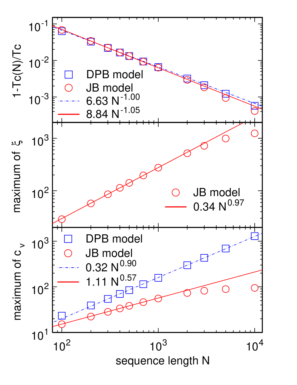
Figure 1:

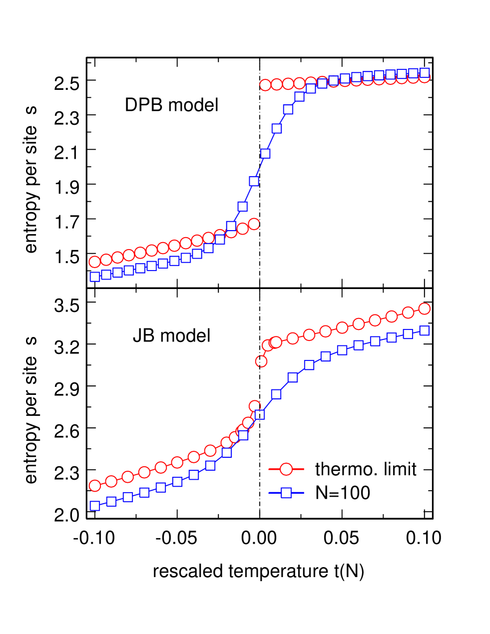
Figure 2:

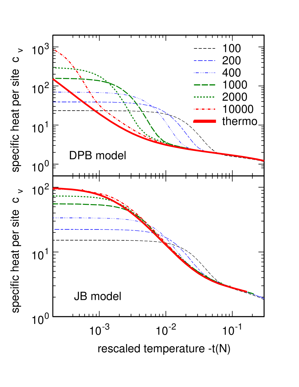
Figure 3:

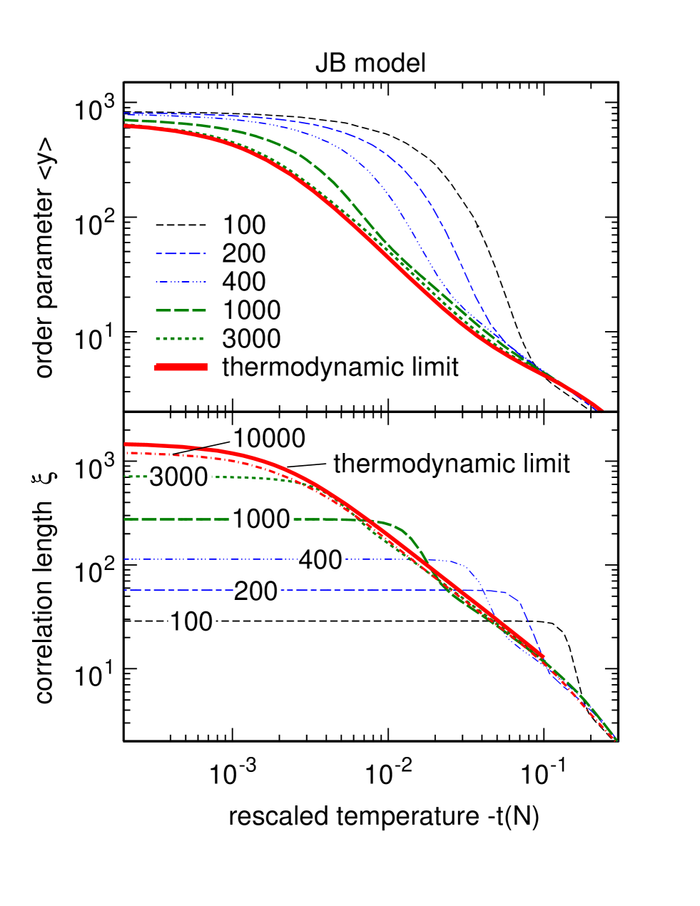
Figure 4:

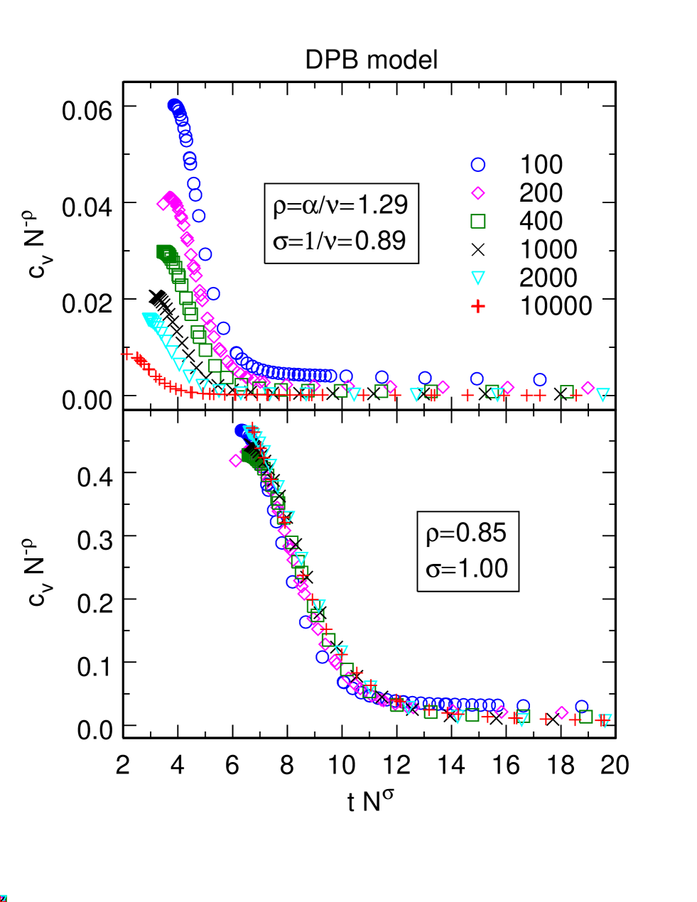
Figure 5:

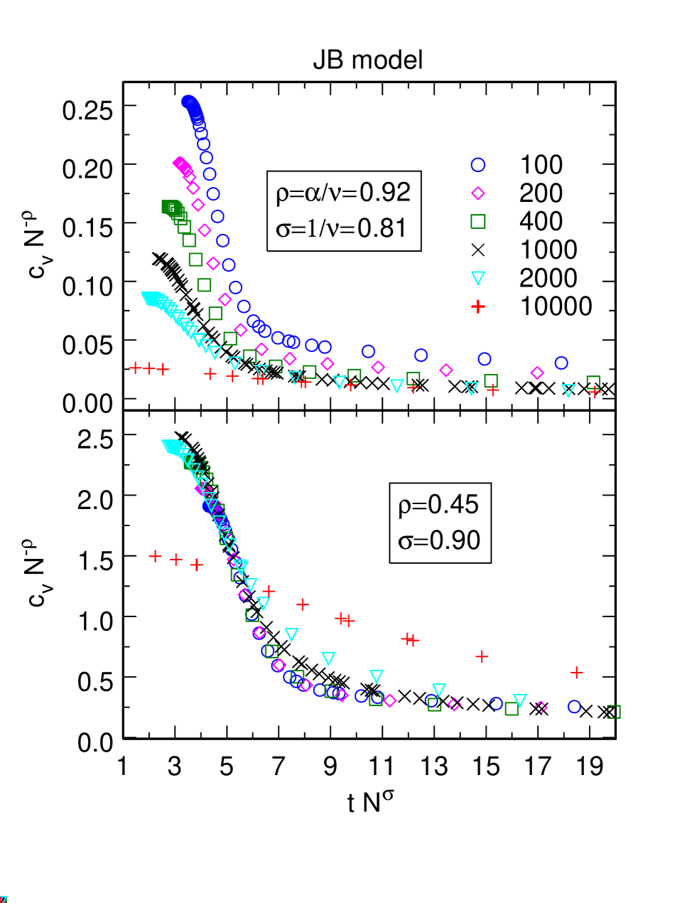
Figure 6:

References

- (1) D.J. Wales and J.P.K. Doye, J. Chem. Phys 103, 3061 (1995)
- (2) P. Borrmann, Oliver Mulken and Jens Harting, Phys. Rev. Lett. 84 3511 (2000)
- (3) O. Mulken, H. Stamerjohanns and P. Borrmann, Phys. Rev. E 64, 047105 (2001)
- (4) D. J. Dean, Int. J. Mod. Phys. 17, 5093 (2001)
- (5) N. A. Alves, J. P. N. Ferrite and U. H. E. Hansmann, Phys. Rev. E 65, 036110 (2002)
- (6) M.E. Fisher and M.N. Barber, Phys. Rev. Lett. 28, 1516 (1972)
- (7) K. Binder and D.P. Landau, Phys. Rev. B 30, 1477 (1984)
- (8) M.S.S Challa, D.P. Landau and K. Binder, Phys. Rev B 34, 1841 (1984)
- (9) K.K. Mon and K. Binder, J. Chem. Phys. 96, 6989 (1992)
- (10) E. Luijten, K. Binder and H.W.J Blöte, Eur. Phys. J. B 9, 289 (1999)
- (11) H.W.J. Blöte and E. Luijten, Europhys. Lett., 38, 565 (1997)
- (12) S. Clar, B. Drossel, K. Schenk and F. Schwabl, Phys. Rev. E 56, 2467 (1997)
- (13) M. Masihi, P.R. King and P. Nurafza, Phys. Rev. E 74, 042102 (2006)
- (14) B. Tadić, Phys. Rev. E 59, 1452 (1999)
- (15) Z. Merdan and R. Erdem, Phys. Letters A 330, 403 (2004)
- (16) S.S. Martinos, A. Malakis and I. Hadjiagapiou, Physica A 355, 393 (2005)
- (17) C. Zhou, D.P. Landau and T.C. Schulthess, Phys. Rev. B 74, 064407 (2006)
- (18) M. Peyrard and A.R. Bishop, Phys. Rev. Lett. 62, 2755 (1989)
- (19) T. Dauxois, M. Peyrard and A.R. Bishop, Phys. Rev. E 47, R44 (1993)
- (20) M. Joyeux and S. Buyukdagli, Phys. Rev. E 72, 051902 (2005)
- (21) S. Buyukdagli and M. Joyeux, Phys. Rev. E 73, 051910 (2006)
- (22) Y.L. Zhang, W.M. Zheng, J.X. Liu and Y.Z. Chen, Phys. Rev. E 56, 7100 (1997)
- (23) V. Privman and M. E. Fisher, J. Stat. Phys. 33, 385(1983)
- (24) K. Binder, M. Nauenberg, V. Privman, A. P. Young, Phys. Rev. B 31, 1498 (1985)
- (25) K. Binder, Ferroelectrics, 73, 43 (1987)