A transactional theory of fluctuations in company size

Abstract

Detailed empirical studies of publicly traded business firms have established that the standard deviation of annual sales growth rates decreases with increasing firm sales as a power law, and that the sales growth distribution is non-Gaussian with slowly decaying tails. To explain these empirical facts, a theory is developed that incorporates both the fluctuations of a single firm’s sales and the statistical differences among many firms. The theory reproduces both the scaling in the standard deviation and the non-Gaussian distribution of growth rates. Earlier models reproduce the same empirical features by splitting firms into somewhat ambiguous subunits; by decomposing total sales into individual transactions, this ambiguity is removed. The theory yields verifiable predictions and accommodates any form of business organization within a firm. Furthermore, because transactions are fundamental to economic activity at all scales, the theory can be extended to all levels of the economy, from individual products to multinational corporations.

I Introduction

In 1931, Gibrat introduced a formal model of market structure based on his Law of Proportionate Effect, which describes the time evolution of business firm size Gibrat ; Sutton1 . There is no unique measure of the size of a company; a firm’s size is frequently defined to be the total annual sales. Gibrat postulated that all firms, regardless of size, have an equal probability to grow a fixed fraction in a given period, i.e., the firm size undergoes a multiplicative random walk. Over appropriately chosen periods, the distribution of the annual fractional size change is approximately Gaussian, independent of the firm size Sutton1 . Gibrat hypothesized that the distribution of firm sizes follows a nonstationary lognormal distribution. Subsequent statistical studies Hart ; Stanley1 have found that the firm-size distribution is well-approximated by a lognormal distribution as predicted. More recent studies Nature96 ; Scaling1 ; Plerou2 ; BottazziPammolli ; Fabritiis ; Gaffeo have also demonstrated three empirical facts incompatible with Gibrat’s hypothesis: (i) Firm growth rates, defined to be the annual change in the logarithm of sales, follow a non-Gaussian distribution with slowly decaying tails, (ii) The standard deviation of growth rates scales as a power law with firm sales, e.g., ${\sigma_{g}\sim{S}^{-\beta}}$, where ${\beta\approx 0.2}$ Nature96 , (iii) The firm size distribution is approximately stationary over tens of years.

A number of models have been proposed to explain these incompatibilities between Gibrat’s theory and the empirical facts. These models decompose each firm into fluctuating subunits Scaling2 ; PRL98 ; Sutton ; BottazziPhysica ; Wyart ; Matia2 ; Fu ; BottazziSecchi ; BottazziSecchi2 , which are usually taken to be management divisions or product lines. While the subunits obey simple dynamics, the aggregate entities approximate the empirically observed statistics. Studies ranging from the gross domestic product (GDP) of countries to the sales of individual products have found comparable scaling laws and non-Gaussian distributions Canning98 ; Lee98 ; BottazziSecchi ; BottazziSecchi2 ; Matia2 ; Fu . While the statistics of GDP growth may be explained in terms of the contributions of individual firms, the firm sales do not obey simple dynamics. Likewise, while firm sales growth may be explained in terms of the contributions from products, products exhibit complex behavior similar to the entire firm Matia2 . Empirically, no economic entity obeying simple dynamics has been identified. In order to reconcile the empirical results of Refs. Canning98 ; Lee98 ; BottazziSecchi ; BottazziSecchi2 ; Matia2 ; Fu with these theoretical models, either a subunit obeying a postulated simple dynamics must be identified, or we must account for the complex nature of the subunits themselves, as illustrated by the hierarchal schematic in Fig. 1.

Figure 1: The GDP of a country is decomposed into the contributions of individual firms. Firms’ contributions are further split by individual products, ad infinitum. Because complex behavior is observed at all scales, models of economies that explain complex behavior in terms of fluctuating subunits must account for the composite nature of the subunits themselves.

Here we develop a theory to explain the observed firm growth statistics that does not invoke an inherently hierarchical model of the economy Nature96 ; Scaling2 ; Buldyrev . We do not make any assumptions about the internal structure of firms. We postulate that the total annual sales of a particular firm can be broken down into a finite sum of individual sales transactions. In our analysis, each firm’s total annual sales is an independent random variable that is characterized by three parameters (see below). Furthermore, these parameters vary randomly from firm to firm. We refer to the set of firms as the population. We define heterogeneity as a measure of the variability of the firms’ parameters within a population.

In Section II, we develop a model of a single firm’s sales. In Section III, we quantify heterogeneity in a population of firms and derive a scaling relationship between firm size and the standard deviation of growth rates. Section IV studies the distribution of annual growth rates for a single firm and approximates the growth distribution generated by a heterogeneous population. Section V uses the scaling analysis presented in Sec. III to illustrate the relationship between the number of products sold by firms and firm sales.

II Model For The Statistics of a Single Firm

We define the size of firm $i$ to be its total annual sales $S_{i}$ which is the sum of $N_{i}$ transactions,

$$S_{i}\equiv T_{i,1}+T_{i,2}+\cdots+T_{i,N_{i}},$$ (1)

where $S_{i}\geq 0$ and $T_{i,k}>0$ are measured in units of currency. We assume both $N_{i}$ and $T_{i,k}$ are independent random variables with finite moments. The total sales $S_{i}$ is then a random variable. Firm $i$ may increase its total sales by increasing its sales volume $N_{i}$, or by selling more expensive products (increasing $T_{i}$). The uncertainties in price and number depend on the nature of the products that a firm sells and the market. We consider Poisson-distributed demand Wu ; Barbour ; Dominey ; NegativeBinomial , where $N_{i}$ is described by a Poisson distribution, and we define

$$Q_{i}\equiv\langle N_{i}\rangle={\rm var}\!\left[N_{i}\right].$$ (2)

With this choice, the size of a firm $S_{i}$ is a random variable with a compound Poisson distribution, the details of which depend on the statistics of the individual transactions $T_{i}$.

For a single firm, the time-averaged mean and variance of sales are denoted by

$$\langle S_{i}\rangle \equiv Q_{i}\;X_{i}$$

$${\rm var}\!\left[S_{i}\right] \equiv Q_{i}\;X_{i}^{2}c_{i}.$$ (3)

where ${X_{i}\equiv\langle T_{i}\rangle}$ is the mean transaction size and ${c_{i}\equiv 1+{\rm var}\!\left[T_{i}\right]/X_{i}^{2}}$ is a measure of the statistical dispersion in transaction sizes. Because of its importance in the subsequent analysis, we introduce the logarithm of the firm size,

$$s_{i}\equiv\log S_{i}.$$ (4)

The log size $s_{i}$ is a random variable that is a function of the random variable $S_{i}$. To simplify the notation, we also introduce the logarithms of the expected number of transactions

$$q_{i}\equiv\log Q_{i},$$ (5)

and the mean transaction size

$$x_{i}\equiv\log X_{i}.$$ (6)

We estimate the first moment of $s_{i}$ by computing the expected value of the Taylor series expansion of Eq. (4) about the mean $\langle S_{i}\rangle$,

$$\langle s_{i}\rangle=\log\left(Q_{i}\;X_{i}\right)-\frac{c_{i}}{2Q_{i}}+\cdots.$$ (7)

In the limit that the number of transactions is large, ${Q_{i}\gg 1}$, we retain only the leading order term,

$$\langle s_{i}\rangle\approx\log\left(Q_{i}\;X_{i}\right)=q_{i}+x_{i}.$$ (8)

The variance of $s_{i}$ is estimated similarly,

$${\rm var}\!\left[s_{i}\right]\approx\frac{Q_{i}\;\langle X_{i}\rangle^{2}c_{i}}{Q_{i}^{2}\langle X_{i}\rangle^{2}}=\frac{c_{i}}{Q_{i}}.$$ (9)

Importantly, the variance in the log size of a firm is inversely proportional to the number of transactions. We combine Eqs. (4), (8), and (9), to compactly express the (approximate) log size of a firm in terms of its mean and standard deviation,

$$\begin{split}s_{i}&=\langle s_{i}\rangle+\left({\rm var}\!\left[s_{i}\right]\,\right)^{1/2}\hat{\eta}\\ &=q_{i}+x_{i}+\left(\frac{c_{i}}{Q_{i}}\right)^{1/2}\hat{\eta},\end{split}$$ (10)

where $\hat{\eta}$ is a random variable that has zero mean and unit variance. Equation (10) expresses the log sales of a particular firm described by the three parameters $q_{i}$, $x_{i}$, and $c_{i}$.

To compute the statistics of sales growth, recall our assumption that the annual sales of firm $i$ is statistically independent of its sales in the previous year. Let $s_{i}$ and $s_{i}^{\prime}$ denote the log size of a firm in two consecutive years, then the annual growth is

$$g_{i}=s_{i}^{\prime}-s_{i}=\left(\frac{c_{i}}{Q_{i}}\right)^{1/2}\left(\hat{\eta}^{\prime}-\hat{\eta}\right).$$ (11)

The growth $g_{i}$ is a random variable with vanishing odd-integer moments and variance given by

$${\rm var}\!\left[g_{i}\right]=\frac{2c_{i}}{Q_{i}}=2c_{i}\exp(-q_{i}).$$ (12)

Thus, we have defined a firm’s total sales to be a sum of a random number of transactions of random size. Each firm is uniquely described by its average sales volume and its transaction sizes, characterized by $q_{i}$, $x_{i}$, and $c_{i}$. The statistical independence of sales from year to year implies that the variance in growth rates, Eq. (12), is a simple function of average sales volume and the transaction size dispersion.

III Quantifying Heterogeneity in the Population of Firms

Prior studies Nature96 ; Scaling1 ; Plerou2 ; BottazziPammolli ; Fabritiis ; Gaffeo examined the statistics of sales growth within a population of firms and found that the standard deviation of growth rates scales as a power law with firm sales, $\sigma_{g}\sim{S}^{-\beta}$, and that the distribution of growth rates is non-Gaussian with slowly decaying tails. Analogously, we examine the statistics of sales growth for a population of firms. We will find that the heterogeneity of firms is fundamental to reproducing the power-law scaling in the standard deviation of growth rates.

We assume that an individual firm’s parameters, $q_{i}$, $x_{i}$, and $c_{i}$, evolve slowly and may be treated as fixed quantities. To introduce heterogeneity within the population, these parameters are sampled from a time-independent distribution Stationary . In the subsequent discussion, we drop the subscript $i$ if a parameter is a random variable that is representative of all firms (not one firm in particular.) Our analysis assumes that the parameter $c$ has finite mean $\langle c\rangle$, and that it is statistically independent of the other firm parameters. The means and variances of the parameters $q$ and $x$ across the population are denoted by

$$\langle q\rangle =m_{q} {\rm var}\!\left[q\right] =\sigma^{2}_{q}$$ (13)

$$\langle x\rangle =m_{x} {\rm var}\!\left[x\right] =\sigma^{2}_{x}.$$ (14)

We take both $q$ and $x$ to be normally distributed within the population, with correlation coefficient $\rho$. The joint probability density function (PDF) of the pair is given by

$$p(q,x)=\frac{\exp\left[-\frac{1}{2}z(1-\rho^{2})^{-1}\right]}{\sqrt{4\pi^{2}\sigma^{2}_{q}\sigma^{2}_{x}(1-\rho^{2})}},$$ (15)

where

$$\begin{split}z\equiv&\frac{(q-m_{q})^{2}}{\sigma^{2}_{q}}+\frac{(x-m_{x})^{2}}{\sigma^{2}_{x}}\\ &\qquad-\frac{2\;\rho\;(q-m_{q})\;(x-m_{x})}{\sigma_{q}\sigma_{x}}.\end{split}$$ (16)

The correlation coefficient depends on the industry: a negative value of $\rho$ implies that firms that sell smaller quantities tend to sell more expensive items. The parameters of Eq. (15) also reflect the fact that firms must minimize inefficiency and risk. Firms with too many transactions have excess overhead, and firms with low volume risk bankruptcy from large sales fluctuations.

Figure 2: Solid ellipses are the level curves of the bivariate distribution given in Eq. (15) with $\rho=0$. Dashed lines show possible configurations of transaction volume and size for firms of various sizes. The arrow indicates that the mean log transaction quantity increases linearly with log size, in agreement with Eq. (19).

We examine the statistics of firms of a fixed mean size, ${s}_{\rm avg}=q+x=const$. As illustrated in Fig. 2, the relationship between total firm sales and transactions imply that statistics that depend on transaction volume $q_{i}$ also depend on the sizes of the firms under consideration. For example, to extend the variance in growth rates given in Eq. (9) to include all firms of a fixed size, we must determine the distribution of $q$ conditioned on ${s}_{\rm avg}$,

$$p(q\,|{s}_{\rm avg})=\frac{p(q,{s}_{\rm avg})}{\int dq\,p(q,{s}_{\rm avg})},$$ (17)

where $p(q,{s}_{\rm avg})$ is a Gaussian PDF that is obtained by substituting the constraint, ${x={s}_{\rm avg}-q}$, into Eq. (15),

$$p(q,{s}_{\rm avg})=p(q,x={s}_{\rm avg}-q).$$ (18)

The quotient of two Gaussian distributions is itself Gaussian. Here, the conditional distribution in Eq. (17) is completely characterized by its conditional mean

$$\begin{split}\langle q\,|{s}_{\rm avg}\rangle\;&=\;2\beta{s}_{\rm avg}\\ &+\frac{(m_{q}-m_{x})\rho\sigma_{q}\sigma_{x}+m_{q}\sigma^{2}_{x}-m_{x}\sigma^{2}_{q}}{u}\;,\end{split}$$ (19)

and conditional variance

$${\rm var}\!\left[q\,|{s}_{\rm avg}\right]=\frac{(1-\rho^{2})\sigma^{2}_{q}\sigma^{2}_{x}}{u},$$ (20)

where

$$\beta=\frac{\sigma^{2}_{q}+\rho\sigma_{q}\sigma_{x}}{2u},\;\;u=\sigma^{2}_{q}+\sigma^{2}_{x}+2\rho\sigma_{q}\sigma_{x}.$$ (21)

We use Eqs. (12), (19), and (20) to find the variance in annual growth rates averaged over all firms of a given log size,

$${\rm var}\!\left[g\,|{s}_{\rm avg}\right]=2\langle c\rangle\exp\left[-\langle q\,|{s}_{\rm avg}\rangle+\frac{{\rm var}\!\left[q\,|\,{s}_{\rm avg}\right]}{2}\right].$$ (22)

This result recovers the empirically observed power-law relationship between firm sales ${S}_{\rm avg}\equiv\exp({s}_{\rm avg})$ and variability in growth rates,

$${\rm var}\!\left[g\,|{S}_{\rm avg}\right]\sim{S}_{\rm avg}^{\,-2\beta}\quad\implies\quad\sigma_{g}\sim{S}_{\rm avg}^{\,-\beta}.$$ (23)

Among all firms of a fixed mean size, we find that the mean number of transactions per year scales as a power law,

$$\langle Q\,|{S}_{\rm avg}\rangle\sim{S}_{\rm avg}^{\,2\beta},$$ (24)

where $Q\equiv{\rm e}^{q}$. A similar calculation for the distribution of the mean transaction size conditioned on firm size also gives a power law,

$$\langle X\,|{S}_{\rm avg}\rangle\sim{S}_{\rm avg}^{1-2\beta},$$ (25)

where $X\equiv{\rm e}^{x}$.

Finally, we note that empirical data are frequently sparse and are binned into large size classes. Appendix A reviews how binning affects the conditional statistics presented in this section.

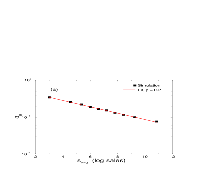
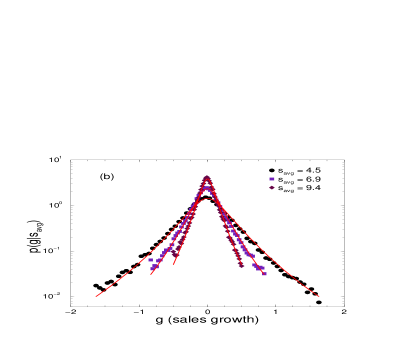
Figure 3: Simulation of 3000 firms for 60 periods with $m_{q}=4.0$, $\sigma^{2}_{q}=2.0$, $m_{x}=3.0$, $\sigma^{2}_{x}=3.0$, $\rho=0$, and constant $c=1.01$. (a) Power-law scaling of the standard deviation of growth rates conditioned on size, and fit to Eq. (23). (b) PDFs of growth rates for firms of three sizes and the corresponding approximate PDFs from Eq. (35).

IV Distribution of Growth Rates

We next address the empirically observed non-Gaussian distribution of sales growth rates Nature96 ; Scaling1 ; Plerou2 ; BottazziPammolli ; Fabritiis ; Gaffeo . In general, a firm’s sales growth distribution $p_{gi}$ depends on a set of firm-specific parameters, which we denote with the vector $\vec{a}_{i}$. For a set of heterogeneous firms $\cal F$, let $p_{a}(\vec{a})$ denote the joint PDF of the parameters. Schematically, the growth rate distribution computed for all firms in the set $\cal F$ is given by

$$\begin{split}\Pi(g|{\cal F})&\equiv\int d\vec{a}\;p_{gi}(g|\vec{a})p_{a}(\vec{a}|{\cal F})\\ &=\int_{0}^{\infty}d\sigma^{2}p(g|\sigma^{2})p(\sigma^{2}|{\cal F}),\end{split}$$ (26)

where the second equality is obtained by integrating over all degrees of freedom except the variance in growth rates, $\sigma^{2}$. For a sufficiently broad variance distribution $p(\sigma^{2}|{\cal F})$, the distribution of growth rates $\Pi(g|{\cal F})$ is non-Gaussian with slowly decaying tails, a typical feature of growth models that incorporate heterogeneity of firms PRL98 ; BottazziPhysica ; Wyart ; Fu ; BottazziSecchi ; BottazziSecchi2 ; Hanssen .

In the present treatment, we note that within a population of firms of fixed average annual sales, there are firms with large numbers of small transactions and vice versa. Because the variance in growth rates is inversely proportional to the number of transactions, the heterogeneity in transaction volume gives rise to a distribution in the variance of firm growth rates. To study the distribution of growth rates beyond the second moment, we must estimate the distribution of a firm’s total sales $S_{i}$.

In actuarial science and operations research literature Dominey ; MART , the distribution of $S_{i}$ has been approximated by the truncated normal, lognormal, and gamma distributions. For analytical convenience, we approximate the compound Poisson distribution of firm sales $S_{i}$ with a gamma distribution. As required by our theory, the gamma distribution admits only nonnegative sales, $S_{i}\geq 0$, and it is asymptotically Gaussian when the number of transactions is large, in agreement with the central limit theorem. The PDF of firm size $S_{i}$ is assumed to be

$$p_{Si}=\frac{S_{i}^{a-1}}{\;b_{i}^{a_{i}}\;\Gamma(a_{i})}\,\exp\left(-\frac{S_{i}}{b_{i}}\right),$$ (27)

where the parameters $a_{i}$ and $b_{i}$ are unique to firm $i$. These parameters are determined by equating the mean and variance to their values given in Eq. (II),

$$\begin{split}\langle S_{i}\rangle&=Q_{i}X_{i}=b_{i}a_{i},\\ {\rm var}\!\left[S_{i}\right]&=Q_{i}X_{i}^{2}c_{i}=b_{i}^{2}a_{i}.\end{split}$$ (28)

We solve Eq. (28) to obtain an expression for $a_{i}$ in terms of the firm parameters,

$$a_{i}=\frac{Q_{i}}{c_{i}}=\frac{\exp(q_{i})}{c_{i}}.$$ (29)

The PDF of a firm’s log size $s_{i}$ follows from Eq. (27),

$$p_{si}=\frac{1}{\;b_{i}^{a_{i}}\;\Gamma(a_{i})}\exp[a_{i}s_{i}-\exp(s_{i})/b_{i}].$$ (30)

Equation (11) defines the growth of a single firm to be the difference of two independent random variables. Therefore, the PDF of single-firm growth rates is given by

$$\begin{split}p_{gi}&=\int_{-\infty}^{\infty}dg^{\prime}\;p_{si}(g^{\prime})\;p_{si}(g^{\prime}+g_{i}),\\ &=\frac{\Gamma(2a_{i}+1)}{a2^{a+1}\Gamma^{2}(a_{i})}\left(1+\cosh g\right)^{-a_{i}}\\ &=\frac{\Gamma(a_{i}+\frac{1}{2})}{2\sqrt{\pi}\;\Gamma(a_{i})}\cosh^{-2a_{i}}\left(\frac{g_{i}}{2}\right).\end{split}$$ (31)

In the case considered here, the distribution of single firm growth rates depends on a single scalar parameter, $a_{i}$. The variance in a firm’s growth rate is given by

$$\begin{split}{\rm var}\!\left[g_{i}\right]=&\langle g_{i}^{2}\rangle=2\Psi_{1}(a_{i})\sim\frac{2}{a_{i}}+\frac{1}{a_{i}^{2}}+\cdots,\\ \end{split}$$ (32)

where $\Psi_{1}$ is the first derivative of the digamma function AbramowitzStegun ,

$$\Psi_{1}(x)=\frac{d}{dx}\Psi(x)=\frac{d^{2}}{dx^{2}}\log\Gamma(x).$$ (33)

In the large-$a_{i}$ limit, we recover the expression for the variance in Eq. (12). This asymptotic agreement is expected because in Sec. II we employed a low-order expansion of the logarithm. Furthermore, because the hyperbolic cosine is asymptotically exponential, the tails of the distribution in Eq. (31) decay exponentially,

The distribution of growth rates for a population must reflect the variability of the parameter $a$ among the firms. Formally, the PDF of growth rates for a population is given by a weighted mixture of the PDFs of single-firm growth rates given in Eq. (31). To express this distribution analytically, we assume negligible variance in the transaction size dispersion, i.e., $c_{i}=c$ is constant. In this case, the distribution of the parameter $a$ is lognormal,

$$p_{a}=\frac{1}{a\sqrt{2\pi V}}\exp\left[-\frac{1}{2V}\bigl{(}\log a\,-\,M\bigr{)}^{2}\right],$$ (34)

where $M\equiv\langle q|{\cal F}\rangle-\log c$ and $V\equiv{\rm var}\!\left[q|{\cal F}\right]$ are determined by the statistics of ${\cal F}$, the set of firms under consideration. For example, to determine the growth rate distribution for the entire population, we use the moments defined in Eq. (13). Alternatively, to compute the distribution of growth rates among firms of fixed size, we use the conditional moments given in Eqs. (19) and (20). In the limit of many transactions, $a\gg 1$, we approximate the PDF of growth rates for a set of heterogeneous firms,

$$\Pi(g|{\cal F})\approx\frac{\exp\left[\bigl{(}4VM+V^{2}-4w^{2}-8w\bigr{)}/\,8V\right]}{\sqrt{4\pi(1+w)}},$$ (35)

where

$$w={\cal W}\left[2V\log\left(\cosh\frac{g}{2}\right){\rm e}^{M+V/2}\right],$$ (36)

and ${\cal W}$ is the Lambert W function Corless , defined by ${\cal W}(x){\rm e}^{{\cal W}(x)}=x$. We give the details of the derivation and an asymptotic analysis of Eq. (35) in Appendix B.

Figure 3 compares Eq. (23) and Eq. (35) to the statistics generated from a simulation of individual firms with annual sales sampled according to Eq. (27). We see that our analysis produces a tent-shaped distribution, consistent with empirical facts Nature96 ; Scaling1 ; Fabritiis .

V The Scaling of Products

Power-law scaling relationships are observed in academic, ecological, technological, and economic systems that relate a measure of size to the number of constituents Plerou1 ; Preston ; MacArthur ; Keitt ; Buldyrev ; Goldenfeld ; Lakhina . For example, the number of different products sold by firms (the constituents) grows as a power law in firm sales (a measure of size), ${{N}\sim{S}^{0.42}}$ Matia2 .

To elucidate the relationship between products and sales, we adopt the notation of Section III. Let $Q_{i}$ denote the number of products within firm $i$ and let $X_{i}$ denote the firm’s total annual sales per product. Because economic conditions are different in different locales and industries, we assume that among all firms, the number of products $Q$ and the mean sales per product $X$ are both lognormally distributed random variables. For convenience, we drop the subscript on the random variables and take the logarithm,

$$S=QX\qquad\rightarrow\qquad s=q+x.$$ (37)

The expression for the joint density of $q$ and $x$ is identical to Eq. (15), except that in this context, the parameters of the distribution reflect aspects of the product portfolios of firms.

From Eqs. (24) and (25), we find that the mean number of products and the mean product size scale as power laws with average firm size,

$$\langle Q\,|{S}_{\rm avg}\rangle \sim {S}_{\rm avg}^{\,2\beta},$$ (38)

$$\langle X\,|{S}_{\rm avg}\rangle \sim {S}_{\rm avg}^{1-2\beta},$$ (39)

where $\beta$ is given in Eq. (21). With a suitable choice of the parameters $\sigma^{2}_{q}$, $\sigma^{2}_{x}$ and $\rho$, one can reproduce the observed power-law scaling relationship between the number of products and firm sales. Moreover, for $\rho=0$ and with $\sigma_{q}^{2}={\cal W}$, and $\sigma_{x}^{2}={\cal D}$, the analysis here is identical to that of Refs. PRL98 ; Matia2 .

VI Discussion

The present model of firm size fluctuations produces a non-Gaussian distribution of growth rates and generates a stationary lognormal distribution of firm sizes, features consistent with empirical studies. Our approach bears similarity to the model proposed in Ref. PRL98 in which a firm is split into subunits that each obey simple dynamics. In the present work, the number of transactions is analogous to the number of subunits, and the transaction size parallels the sizes of the subunits within a firm. The model of Ref. PRL98 postulates a complex internal structure within a firm. In contrast, our approach decomposes a firm’s sales into the individual transactions that occur in a year.

Because transactions are well-defined measurable quantities, the assumptions and predictions of the theory are verifiable. In practice, correlations between transactions invalidate our assumption that the number of transactions $N_{i}$ follows a Poisson distribution. Indeed, transactions within a firm can be regrouped to remove correlations. Because these uncorrelated groups satisfy the assumptions of our model, we conclude that a Poisson-distributed number of transactions is not strictly necessary to obtain the results presented here. To retain our transactional framework, one can extend the model of a single firm’s statistics described in Section II to account for correlations between transactions at the expense of additional parameters NegativeBinomial . Independent of the statistical details, most measures of microeconomic and macroeconomic consumption tally individual transactions and are therefore amenable to the transactional approach presented here. Figuratively speaking, transactions are the ‘atoms’ of economic activity: they are discrete and are the basis of economies of all scales, from the individual to the national.

Using our approach, we studied the relationship between the number of different products sold by firms and total sales receipts. We found that differences between firms could account for the reported scaling relationship between the two quantities, $\langle Q\,|{S}_{\rm avg}\rangle\sim{S}_{\rm avg}^{\,2\beta}$. Our analysis applies to many systems where two distinct measures of size are related by a proportionality constant that varies because of economic, environmental, and other accidental circumstances. When the relationship between the measures is weak, the population is heterogeneous and non-trivial power laws emerge Buldyrev . For example, both transaction volume and total sales quantify the size of a firm, but no strict universal proportionality between these quantities exists. In this case, Eq. (24) predicts a power-law relationship between the quantities. In ecology, both island surface area and number of species quantify island size: islands with greater area generally harbor more species. However, the mix of species and the number distinct niches varies from island to island. In agreement with our hypothesis, empirical studies show that the number of species scales as a power law with island area $S\sim A^{z}$, $z\approx 0.2$ Preston ; MacArthur ; Goldenfeld . Other studies have found that the density of Internet routers scale as a power law with population density, $R\sim P^{\alpha}$, $\alpha\approx 1.4$ Lakhina . In our treatment, the particular exponent is a function of the heterogeneity in the Internet architecture deployed within a study region.

In summary, we have presented a theory of firm size fluctuations that explains a number of reported statistics in economics. The analysis also represents an important null hypothesis because it suggests that some emergent statistics are a consequence of heterogeneity in the population of firms. For these systems, understanding and quantifying heterogeneity seems to be the central problem in understanding macroscopic firm statistics.

VII Acknowledgments

We acknowledge discussions with K. Matia, K. Yamasaki, F. Pammolli, and M. Riccaboni. We also thank S. Sreenivasan and George Schweiger for their reading of the manuscript and insightful suggestions. We thank DOE Grant No. DE-FG02-95ER14498 and the NSF for support.

Appendix A Statistics of Binning

Frequently, empirical analysis of data cannot select a significant set of firms of a fixed size. The usual remedy is to bin by selecting data within a range of sizes. Because the range may be large, the conditional statistics may change. For example, we examine the conditional mean and variance of $q$, for the subset of firms in the bin $s_{\min}\leq{s}_{\rm avg}\leq s_{\max}$. Within the bin, the distribution of ${s}_{\rm avg}$ is a complicated function of $s_{\min}$ and $s_{\max}$. We denote the average of the log mean size of firms within the bin by $\langle{s}_{\rm avg}\,|B\rangle$, the corresponding variance within the bin is denoted by ${\rm var}\!\left[{s}_{\rm avg}\,|B\right]$. The conditional expectation $\langle q\,|{s}_{\rm avg}\rangle$ given in Eq. (19) is linear in ${s}_{\rm avg}$, consequently, binning has no impact on the calculation of the conditional first moment. The variance of $q$ for the set of firms within the bin is given by

$${\rm var}\!\left[q\,|B\right]={\rm var}\!\left[q\,|\langle{s}_{\rm avg}\,|B\rangle\right]+4\beta^{2}{\rm var}\!\left[{s}_{\rm avg}\,|B\right],$$ (40)

where ${\rm var}\!\left[q\,|\langle{s}_{\rm avg}\,|B\rangle\right]$ is defined in Eq. (20). The above relationship implies that Eq. (23) holds only when we have binned firms such that the variance in firms’ log mean size in each bin, ${\rm var}\!\left[{s}_{\rm avg}\,|B\right]$, is a constant. Furthermore, because the mean and variance of $q$ is reflected in the parameters $M$ and $V$ in Eq. (34), this implies that the distribution of growth rates also has a non-trivial dependence on bin width.

Appendix B Estimation of the Growth Rate Distribution

The formal expression for the PDF of growth rates for a set of firms $\cal F$ follows from Eqs. (31) and (34),

$$\Pi(g|{\cal F})=\int da\frac{{\rm e}^{-[\log a-M]^{2}/2V}}{a\sqrt{2\pi V}}\frac{\Gamma(a+\frac{1}{2})}{2\sqrt{\pi}\;\Gamma(a)}\cosh^{-2a}\!\!\left(\frac{g}{2}\right).$$

In equilibrium, viable firms cannot sustain large sales fluctuations, so $a\gg 1$ and $M\gg V$. We replace the integrand with its leading-order term in the asymptotic expansion in $a$ and perform a change of variables,

$$\begin{split}\Pi(g|{\cal F})&\approx\int da\frac{{\rm e}^{-[\log a-M]^{2}/2V}}{a\sqrt{2\pi V}}\frac{\sqrt{a}}{2\sqrt{\pi}}\cosh^{-2a}\!\!\left(\frac{g}{2}\right)\\ &=\int dz\frac{{\rm e}^{z/2-[z-M]^{2}/2V}}{2\pi\sqrt{2V}}\left[\cosh\;\frac{g}{2}\right]^{-2\exp(z)}.\end{split}$$ (41)

We approximate the second integral in Eq. (41) using the Laplace method to obtain Eq. (35).

To examine the large-$g$ behavior of Eq. (35), note that the Lambert W function is asymptotically logarithmic, ${\cal W}(x)\sim\log(x)$. We set $w\rightarrow\log g+\log V+M+V/2$ in Eq. (35) to obtain,

$$\Pi(g|{\cal F})\sim\frac{\exp[-\log^{2}\!g\,/\,2V]}{\sqrt{\gamma_{0}V\,+\,\log g\;}}\;g^{-\gamma_{0}},\\$$ (42)

where the exponent $\gamma_{0}$ is given by,

$$\gamma_{0}=\frac{1}{2}+\frac{1+M+\log V}{V}.$$ (43)

For finite $V$, the tail of the distribution of growth rates $\Pi(g)$ decays slower than an exponential, in agreement with empirical studies.

References

- (1) R. Gibrat, Les Inégalités Economiques (Sirey, Paris, 1933).
- (2) J. Sutton, J. of Econom. Lit. 35, 40 (1997).
- (3) P. E. Hart and S. J. Prais, J. Roy. Stat. Soc. 119, 150 (1956).
- (4) M. H. R. Stanley, S. B. Buldyrev, R. N. Mantegna, S. Havlin, M. A. Salinger, and H. E. Stanley, Econ. Lett. 49, 453 (1995).
- (5) M. H. R. Stanley, L. A. N. Amaral, S. V. Buldyrev, S. Havlin, H. Leschhorn, P. Maass, M. A. Salinger, and H. E. Stanley, Nature 379, 804-806 (1996).
- (6) L. A. N. Amaral, S. V. Buldyrev, S. Havlin, H. Leschhorn, P. Maass, M. A. Salinger, H. E. Stanley, and M. H. R. Stanley, J. Phys. I (France) 7, 621 (1997).
- (7) V. Plerou, P. Gopikrishnan, L. A. N. Amaral, M. Meyer, and H. E. Stanley, Phys. Rev. E 60 6519 (1999).
- (8) G. Bottazzi, G. Dosi, M. Lippi, F. Pammolli, and M. Riccaboni, Int. J. Ind. Org. 19, 1161 (2001).
- (9) G. De Fabritiis, F. Pammolli, and M. Riccaboni, Physica A 324, 38 (2003).
- (10) E. Gaffeo, M. Gallegati, and A. Palestrini, Physica A 324, 117 (2003).
- (11) S. V. Buldyrev, L. A. N. Amaral, S. Havlin, H. Leschhorn, P. Maass, M. A. Salinger, H. E. Stanley, and M. H. R. Stanley, J. Phys. I France 7, 635 (1997).
- (12) L. A. N. Amaral, S. V. Buldyrev, S. Havlin, M. A. Salinger, and H. E. Stanley, Phys. Rev. Lett. 80, 1385 (1998).
- (13) J. Sutton, Physica A 312, 577 (2002).
- (14) G. Bottazzi and A. Secchi, Physica A 324, 213 (2003).
- (15) M. Wyart and J.-P. Bouchaud, Physica A 326, 241 (2003).
- (16) K. Matia, D. Fu, S. V. Buldyrev, F. Pammolli, M. Riccaboni, and H. E. Stanley, Europhys. Lett. 67, 498 (2004).
- (17) D. Fu, F. Pammolli, S. V. Buldyrev, M. Riccaboni, K. Matia, K. Yamasaki, and H. E. Stanley,
- (18) G. Bottazzi and A. Secchi, Industrial and Corporate Change 15, 847 (2006).
- (19) G. Bottazzi and A. Secchi, RAND Journal of Economics 37, 234 (2006).
- (20) D. Canning, L. A. N. Amaral, Y. Lee, M. Meyer, and H. E. Stanley, Economics Letters 60, 335 (1998).
- (21) Y. Lee, L. A. N. Amaral, D. Canning, M. Meyer, and H. E. Stanley, Phys. Rev. Lett. 81 3275 (1998).
- (22) L. S.-Y. Wu, The Statistician 37, 141 (1988).
- (23) A. D. Barbour and C. Chryssanphinou, Ann. Appl. Probab. 11, 964 (2001).
- (24) One generalization is to let be drawn from a negative binomial distribution. In this case, we obtain a more general model at the expense of an additional parameter. More rigourous approaches are presented in Ref. MART .
- (25) M. J. G. Dominey and R. M. Hill, Int. J. Production Economics 92, 145 (2004).
- (26) R. Kaas, M. Goovaerts, J. Dhaene, and M. Denuit, Modern Actuarial Risk Theory (Springer, New York, 2005).
- (27) M. Abramowitz and I. A. Stegun, Handbook of Mathematical Functions (Dover, New York, 1972).
- (28) The assumption of a time-independent distribution is incompatible with changes in demand, technological innovation, and political and economic climate. We assume that this assumption is a reasonable approximation for statistics gathered over tens of years.
- (29) R. M. Corless, G. H. Gonnet, D. E. G. Hare, D.J. Jeffrey, and D. E. Knuth, Adv. Comput. Math. 5, 329 (1996).
- (30) A. Hanssen and T. A. Øigȧrd, IEEE International Conference on Acoustics, Speech, and Signal Processing, Vol. 6, pp. 3985-3988, Salt Lake City, UT, May 2001.
- (31) V. Plerou, L. A. N. Amaral, P. Gopikrishnan, M. Meyer, and H. E. Stanley, Nature 400, 433 (1999).
- (32) F. W. Preston, Ecology 43, 185 (1962).
- (33) R. H. MacArthur and E. O. Wilson, The Theory of Island Biogeography (Princeton University Press, Princeton, New Jersey, 1967).
- (34) T. H. Keitt and H. E. Stanley, Nature 393, 257 (1998).
- (35) S. V. Buldyrev, N. V. Dokholyan, S. Erramilli, M. Hong, J. Y. Kim, G. Malescio, and H. E. Stanley, Physica A 330, 653 (2003).
- (36) H. Garcia Martin and N. Goldenfeld, Proc. Nat. Acad. Sci. 103, 10310 (2006).
- (37) A. Lakhina, J. W. Byers, M. Crovella, and I. Matta, IEEE J. on Sel. Areas Commun. 21, 934 (2003).