Accuracy of one-dimensional collision integral in the rigid spheres approximation

Abstract

The accuracy of calculation of spectral line shapes in one-dimensional approximation is studied analytically in several limiting cases for arbitrary collision kernel and numerically in the rigid spheres model. It is shown that the deviation of the line profile is maximal in the center of the line in case of large perturber mass and intermediate values of collision frequency. For moderate masses of buffer molecules the error of one-dimensional approximation is found not to exceed 5%.

1 Introduction

Modern high resolution spectrometry of molecular gases requires a precise knowledge of spectral lines shapes. The present-day experimental techniques have reached so high precision and accuracy, that models describing line shapes have to take into account such fine effects as velocity dependence of collisional width and shift, correlation between velocity changing and phase shifting collisions, finite impact time, and radiation relaxation. The profile of an isolated spectral line is usually obtained by solving quantum kinetic equation for the off-diagonal element of the density matrix describing the active gas [22]. The essence of any model describing line shapes is the way it accounts for the collisions of radiator and perturber molecules. In principle, in the impact approximation the term accounting for collisions can be obtained by averaging the corresponding transition frequencies over velocities of the buffer molecules, as described in [21]. The kinetic equation is a three-dimensional integral equation. Actually, it can be reduced to a two-dimensional, because the problem has an axial symmetry with respect to the wave propagation direction. Due to computational difficulties, this ab initio approach is rarely used for approximating experimental line shapes. Instead, most works on this subject utilize various simplified models of collision term. The simplest of these models lead to one-dimensional equations. They are the strong collisions [15], the weak collisions [7] and the Keilson-Storer [9] models. The more complicated ones, such as the rigid spheres [10] and “kangaroo” [5] models yield 3D equations.

The work [10], in which the first attempt was made to proceed from the simplest models to a more complicated one introduced a combined approach. The rigid spheres collision kernel, which was analyzed in this work, leads to a 3D integral equation. However, in order to simplify the numerical calculations, the kinetic equation was reduced to a 1D integral equation by averaging the kernel over the transverse components of velocity with Maxwellian weight. This reduction is equivalent to adopting the assumption that the distribution of the off-diagonal element of the density matrix over the transverse (to the wave propagation direction) velocity components is Maxwellian. In other words, this approximation, known as the one-dimensional model, neglects the transfer of nonequilibrium created by the interaction with the light wave to the distribution over the transverse velocities. Later the 1D approximation was used in [21] and [3] to analyze general aspects of influence of collisions on spectral line profiles. The 1D approximation in the rigid spheres model was utilized in [11] to fit the experimental line shapes. The line shapes in 1D rigid spheres were comprehensively studied and compared to other models in [23].

In our time the calculation of a line shape in the rigid spheres model can be performed on a usual desktop computer without utilizing 1D approximation. However, it may still become useful when improvement of precision of experimental measuring of spectral lines profiles will persuade researchers to turn to even more realistic models, with kernels describing simultaneously dephasing and velocity-changing collisions.

The investigation of precision of the 1D approximation is also motivated by the following. It has been pointed out recently [24] that probably much of the disagreement between theoretical and experimentally measured line shapes could be removed if the calculation of dephasing term was performed using the correct velocity distribution of the off-diagonal element of the density matrix instead of Maxwell’s distribution. The understanding of to what extent this distribution really differs from equilibrium is required to clarify this problem. The answer to the question, how much of the non-equilibrium is transported to the distribution over transverse velocities, could contribute to such understanding.

The question of precision of the 1D approximation was first studied quantitatively in [19]. In this article the problem was studied in the so-called ”kangaroo” model. The accuracy of the 1D approximation was found to be good. Later the same result was extended to the accuracy of 1D approximation in describing the light induced drift effect [16] in the “kangaroo” model. This research was continued in [17] with special attention to Dicke narrowing effect and gave the same result. The overall conclusion of these three articles regarding 1D approximation is, its accuracy is high and it can be used for studying a wide range of problems both in linear and nonlinear spectroscopy. This thorough analysis does not seem quite general and comprehensive. The mere fact that the three mentioned simple models of collision integral lead to 1D kinetic equation (and so the 1D approximation is precise for them) shows that the accuracy of this approximation is determined by some fine properties of the collision integral. Thus the model of collision integral which is used to study this problem should be more realistic than the degenerate (in the sense that it has infinite number of eigenvectors with zero eigenvalue) collision kernel of the “kangaroo” model. It seems more appropriate to utilize the rigid spheres model for this purpose. This model’s collision kernel is obtained by direct averaging of the cross-section (though for a not very realistic potential), so it has many realistic features. Another factor that draws attention to this model is that it is often used (in combination with other terms accounting for collisional broadening and shifting) to fit experimentally obtained profiles, e.g. in [25, 14].

The goal of the present work is to study the precision and the area of applicability of the 1D approximation quantitatively in the rigid spheres model. This paper is organized as follows. In the next section the rigid spheres model is briefly described and the 1D approximation is introduced. Section 3 is devoted to analysis of the accuracy of 1D model in several limiting cases. The results of numerical calculations in the rigid spheres model are presented and discussed in Section 4. The conclusions are drawn in the last section.

2 Basic equations

2.1 The rigid spheres model

Let us briefly remind the basic equations defining spectral line shapes, following [21]. The gas interacting with radiation can be described in terms of density matrix $\hat{\rho}(\mathbf{v})$, depending on velocity $\mathbf{v}$. Let the wave’s frequency be close to resonance with the transition between the levels $m$ and $n$. Then, in the resonance approximation, the line shape is defined by the off-diagonal element $\rho_{mn}(\mathbf{v})$. Below we will denote it as $\rho(v)$ without indices. It is governed by the following master equation:

$$\left(-\textrm{i}\omega+\textrm{i}\mathbf{kv}+\Gamma\right)\rho(\mathbf{v},\omega)=W(\mathbf{v})+\mathbf{\hat{S}}\rho(\mathbf{v},\omega),$$ (1)

here $\omega$ is the detuning of the wave’s frequency from the resonance, $\mathbf{k}$ is the wave vector of the light wave, $W(\mathbf{v})$ is Maxwell’s distribution, $\Gamma$ is the relaxation constant, $\mathbf{\hat{S}}$ is the collision operator. The line shape is given by the formula

$$I(\omega)=\frac{1}{\pi}\;\textrm{Re}\int\rho(\mathbf{v})\;d^{3}\mathbf{v}.$$ (2)

The relaxation constant $\Gamma$ is assumed to be velocity-independent. In this case, it influences the line shape in the following way:

$$I(\omega,\Gamma)=\int I(\omega^{\prime},0)\;\;\frac{\Gamma}{\Gamma^{2}+(\omega-\omega^{\prime})^{2}}\;\frac{d\omega^{\prime}}{\pi},$$ (3)

that is, the line shape is a convolution of the form of the line in the absence of $\Gamma$ with a Lorentzian profile. Thus the relaxation tends to conceal any details of the collision integral, including the differences between the initial 3D collision integral and its 1D analog. In this paper we consider equation (1) only with $\Gamma=0$, because in this case the inaccuracy of the 1D approximation is most noticeable.

We consider the collision operator $\mathbf{\hat{S}}$ in the impact approximation and also assume that the cross section of scattering of active molecule by buffer gas molecules is independent of the molecule’s state (full phase memory). Under these assumptions the collision integral takes the form

$$\mathbf{\hat{S}}\rho(\mathbf{v})=\int A(\mathbf{v},\mathbf{v}^{\prime})\rho(\mathbf{v}^{\prime})d\mathbf{v}^{\prime}-\nu(\mathbf{v})\rho(\mathbf{v}).$$ (4)

The function $A$ is the collision kernel, $\nu$ is the scattering-out frequency. Owing to the assumption we made, the functions $\nu$ and $A$ are bound by the following relation:

$$\nu(\mathbf{v})=\int A(\mathbf{v}^{\prime},\mathbf{v})\;d\mathbf{v}^{\prime}.$$ (5)

It can be inferred from equations (4) and (5) that

$$\int d\mathbf{v}\;\mathbf{\hat{S}}\;\rho=0$$ (6)

for any $\rho(\mathbf{v})$. Another general property of the collision integral (4) can be derived from the detailed balancing principle:

$$A(\mathbf{v},\mathbf{v}^{\prime})W(\mathbf{v}^{\prime})=A(\mathbf{v}^{\prime},\mathbf{v})W(\mathbf{v}).$$ (7)

Taking into account the definition (5) of $\nu$ we obtain

$$\mathbf{\hat{S}}W(\mathbf{v})=0.$$ (8)

Below we utilize the rigid spheres (or ”billiard balls”) collision kernel in all the calculations requiring a definite collision integral. In this model the differential cross section of scattering is considered to be independent of relative velocity and equal to $d\sigma/do=a^{2}/4$, here $a$ is the effective sum of radii of active and buffer molecules, and $do$ is the element of solid angle. The collision kernel in the rigid spheres model is obtained by averaging the probability of a collision, changing the velocity of active molecule from $\mathbf{v}$ to $\mathbf{v}^{\prime}$, over the velocities of buffer molecules. Its explicit form is [21, 10]

$$A_{\mbox{\tiny{\bf RS}}}(\mathbf{v}|\mathbf{v^{\prime}})=\frac{N_{b}\,v_{bT}}{\sqrt{\pi}}\;\frac{a^{2}}{\Delta^{2}\zeta}\;\exp\left[-\left(\frac{\bm{\zeta}(\bm{\zeta}+\frac{2\mu}{M}\mathbf{{v^{\prime}}})}{\zeta\Delta}\right)^{2}\;\right],$$ (9)

here $m$ is the mass of the buffer molecule, $M$ is the mass of the active molecule, $\bm{\zeta}=\mathbf{v}-\mathbf{v^{\prime}}$, $\Delta=\frac{2\mu}{M}\mathrm{v}_{bT}$, $\mathrm{v}_{bT}=\mathrm{v}_{T}\left/\sqrt{\beta}\right.$ is the most probable velocity of the buffer molecule, $\beta=m/M$ is the mass ratio, $\mu={mM}\!\left/{\left(m+M\right)}\right.$ is the reduced mass. The kernel (9) has a singularity $1/\zeta$ caused by the energy conservation. The absence of such singularity in most phenomenological kernels corresponds to suppression of small angle scattering. The kernel (9) explicitly depends on $\beta$ and demonstrates correct behavior in the limits $\beta\rightarrow 0$ and $\beta\rightarrow\infty$.

The scattering-out term in this model has the form:

$$\nu_{\mbox{\tiny{\bf RS}}}(\mathrm{v})=\frac{N_{b}v_{bT}a^{2}}{2}\left(\frac{2}{\sqrt{\pi}}\;e^{-z^{2}}+\left[2z+\frac{1}{z}\right]\mbox{Erf}(z)\right),$$

where $\mbox{Erf}(z)=\frac{2}{\sqrt{\pi}}\int\limits^{z}_{0}e^{-x^{2}}\,dx$ denotes the error function [2] and $z=\mathrm{v}\left/\mathrm{v}_{bT}\right.$.

2.2 The one-dimensional model

Equation (1) is a two-dimensional (due to axial symmetry of the problem) integral equation. Its direct numerical solution presents certain difficulties, so various simplified models are widely used. One of such models is so-called one-dimensional approximation. In this models the dependence of $\rho(\mathbf{v})$ on the transverse components of the velocity $\mathbf{v}$ is considered to be Maxwellian. This assumption allows to write instead of (1) an equation for dependance of $\rho$ on the longitudinal velocity $\mathrm{v}_{z}$:

$$\left(-i\omega+ik\mathrm{v}_{z}+\Gamma\right)\rho(\mathrm{v}_{z})=\\ =-\nu^{1D}\rho(\mathrm{v}_{z})+\int A^{1D}(\mathrm{v}_{z}|\mathrm{v}^{\prime}_{z})\rho(\mathrm{v}^{\prime}_{z})d\mathrm{v}^{\prime}_{z},$$ (10)

where

$$A^{1D}(\mathrm{v}_{z},\mathrm{v}^{\prime}_{z})=\int A(\mathbf{v}|\mathbf{v^{\prime}})\frac{e^{-\mathbf{v}^{\prime 2}_{\perp}/\mathrm{v}_{T}^{2}}}{\pi}d^{2}\mathbf{v}_{\perp}d^{2}\mathbf{v}^{\prime}_{\perp},$$ (11)

and

$$\nu^{1D}(\mathrm{v}_{z})=\int A^{1D}(\mathrm{v}^{\prime}_{z},\mathrm{v}_{z})\;d\mathrm{v}^{\prime}_{z}.$$ (12)

Here $A^{1D}$ and $\nu^{1D}$ are one-dimensional collision kernel and scattering-ou t frequency, $\mathbf{v}_{\perp}$ and $\mathbf{v}^{\prime}_{\perp}$ are the components of velocity, orthogonal to the wave propagation direction, and $\mathrm{v}_{T}$ is the most probable velocity of active molecules $\mathrm{v}_{T}=\sqrt{2mT}$.

In the 1D approximation the rigid spheres collision kernel (9) is reduced to

$$A^{1D}_{\mbox{\tiny{\bf RS}}}(\mathrm{v}_{z},\mathrm{v}_{z}^{\prime})=\\ =\pi N_{b}a^{2}\mathrm{v}_{T}\frac{\beta+1}{4\beta}\left\{e^{\mathrm{v}_{z}^{\prime 2}-\mathrm{v}_{z}^{2}}\left[1+\sigma\mbox{Erf}\left(\frac{\beta-1}{2\sqrt{\beta}}\mathrm{v}_{z}+\frac{\beta+1}{2\sqrt{\beta}}\mathrm{v}_{z}^{\prime}\right)\right]+\right.\\ \left.+1-\sigma\mbox{Erf}\left(\frac{\beta+1}{2\sqrt{\beta}}\mathrm{v}_{z}+\frac{\beta-1}{2\sqrt{\beta}}\mathrm{v}_{z}^{\prime}\right)\right\},$$ (13)

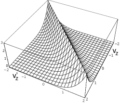
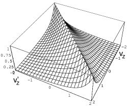
where $\sigma=\mbox{sign}(\mathrm{v}_{z}-\mathrm{v}_{z}^{\prime})$. This kernel as a function of the initial and final velocity is presented in fig. 1. In order to make this figure more illustrative we plot “symmetrized” kernel $A^{1D}(\mathrm{v}_{z},\mathrm{v}^{\prime}_{z})exp\left[\left(\mathrm{v}_{z}^{2}-\mathrm{v}_{z}^{\prime 2}\right)/2\right]$. This function is a symmetric function with respect to transformation $\mathrm{v}_{z}\leftrightarrow\mathrm{v}^{\prime}_{z}$. At small perturber mass $\beta\ll 1$, Fig. 1, the kernel function has sharp peak near $\mathrm{v}_{z}^{\prime}=\mathrm{v}_{z}$, which means that the small velocity change is the most probable. For comparable perturber $\beta\sim 1$, the peak broadens. For heavy perturber $\beta\gg 1$, Fig. 1, the additional ridge near $\mathrm{v}_{z}^{\prime}=-\mathrm{v}_{z}$ arises corresponding to elastic backward scattering on a perturbing molecule.

Figure 1: Shape of the “symmetrized” kernel $A^{1D}(\mathrm{v}_{z},\mathrm{v}^{\prime}_{z})\exp\left[\left(\mathrm{v}_{z}^{2}-\mathrm{v}_{z}^{\prime 2}\right)/2\right]$ at different $\beta=1/5(a),1(b),5(c)$.

Integrating expression (13) over $\mathrm{v}_{z}$, we obtain the out-scattering frequency of 1D rigid spheres model:

$$\nu^{1D}_{\mbox{\tiny{\bf RS}}}(\mathrm{v}_{z})=\pi N_{b}a^{2}\mathrm{v}_{T}\left(\mathrm{v}_{z}\;\mbox{Erf}(\sqrt{\beta}\mathrm{v}_{z})+\frac{e^{-\beta\mathrm{v}_{z}^{2}}}{\sqrt{\pi\beta}}+\frac{1+\beta}{\beta}\;e^{\mathrm{v}_{z}^{2}}\int_{\mathrm{v}_{z}}^{\infty}\mbox{Erf}(\sqrt{\beta}t)\;e^{-t^{2}}\;dt\right).$$ (14)

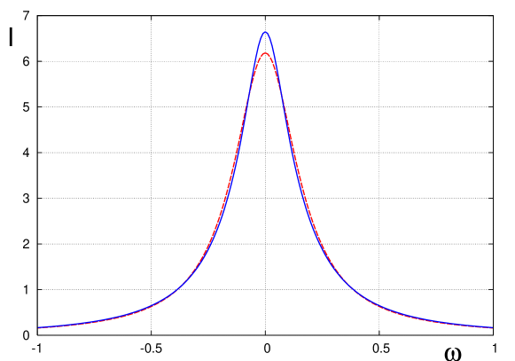
The line shape in the 1D rigid spheres model can differ significantly from its shape in full rigid spheres model, as it is demonstrated in Fig. 2. It can be seen on this picture, that the 1D line almost coincides with 3D in the wings of the line, but goes considerably lower in its center. In the next section we will analyze this difference in several limiting cases.

Figure 2: Shape of the spectral line $I(\omega)$ in the rigid spheres model at $\beta=100$, $\nu_{d}=3k\mathrm{v}_{T}$. The solid line corresponds to the rigid spheres approximation, the dashed line corresponds to its 1D approximation.

The essence of the 1D model is the assumption that the transfer of non-equilibrium to the distribution of $\rho$ over the transverse components of velocity is negligible. Figure 3 demonstrates, that this transfer is not weak in general case.

\psfrag{long}{\Large$v_{z}$}\psfrag{trans}{\Large$v_{\bot}$}\includegraphics[width=195.12767pt]{ill1bw.eps}

\psfrag{long}{\Large$v_{z}$}\psfrag{trans}{\Large$v_{\bot}$}\includegraphics[width=195.12767pt]{ill2bw.eps}

Figure 3: Distribution of the value $\rho(\mathbf{v})/W(\mathbf{v})$ over longitudinal and transverse components of velocity in the rigid spheres model at $\omega=0$ and $\Gamma=0.5\,k\mathrm{v}_{T}$. The first plot (a) corresponds to absence of collisions. The second plot (b) corresponds to the case $\beta\rightarrow\infty$, $C=3$ (see section 3.4).

Fig. 3 (a) represents the distribution of $\rho(\mathbf{v})$, divided by Maxwellian distribution, in absence of collisions. It can be seen that the dependence on transverse velocity is uniform. Fig. 3 (b) represents the distribution of the same value in presence of the collision integral. The dependence on the transverse velocity becomes strongly nonuniform. Thus it could be expected that the impact of transfer of non-equilibrium on line shapes would be also strong. However, as it will be shown, in most cases it turns out to be numerically small.

3 The limiting cases

3.1 The wings of spectral line profile

Let us at first consider the spectral wings of the line. Note that the calculations below take into account only rigid spheres elastic collisions and ignore other effects determining the far wings. It is convenient to turn to the time domain for this purpose and to introduce the Fourier transform of $\rho(\mathbf{v},\omega)$

$$\rho(\mathbf{v},t)=\int\rho(\mathbf{v},\omega)\;e^{-\textrm{i}\omega t}\;\frac{d\omega}{2\pi}.$$ (15)

The function $\rho(\mathbf{v},t)$ satisfies the following evolution equation:

$$\left(\frac{\partial}{\partial t}+\textrm{i}\mathbf{kv}\right)\rho(\mathbf{v},t)=\mathbf{\hat{S}}\rho(\mathbf{v},t)+W(\mathbf{v})\delta(t).$$ (16)

This equation has only one solution that tends to zero at $t\rightarrow\pm\infty$. Let us define the autocorrelation function $\Psi(t)$ as

$$\Psi(t)=\int\rho(\mathbf{v},t)\;d\mathbf{v}.$$ (17)

This function is different from usually used function $\Phi(t)$ [21] in the following way: $\Psi$ is an even function of $t$, while $\Phi$ is zero at negative values of $t$. It is evident from (15), (16) and (17) that $\Psi(t)$ is a real continuous even function connected with the line shape by the Fourier transform

$$I(\omega)=\frac{1}{\pi}\int\Psi(t)e^{i\omega t}dt.$$ (18)

The asymptote of $I(\omega)$ at $\omega\rightarrow\infty$ is determined by the discontinuities of the derivatives of $\Psi(t)$ at $t=0$. Using (16) and taking into account (8) and (6) we find that (in the absence of $\Gamma$) the lowest order of derivative of $\Psi(t)$ having a jump at $t=0$ is third. Thus the asymptote of $I(\omega)$ can be written as

$$I(\omega)=\frac{1}{\pi\omega^{4}}\int d\mathbf{v}\;\mathbf{k}\mathbf{v}\;\mathbf{\hat{S}}\;\mathbf{k}\mathbf{v}\;W+O(1/\omega^{6})\quad\mbox{at}\;\omega\rightarrow\pm\infty.$$ (19)

In order to obtain the value of the coefficient of the dominant term of this asymptote we have to substitute the definition (4) of $\mathbf{\hat{S}}$ into Eq.(19) with some specific kernel $A(\mathbf{v},\mathbf{v}^{\prime})$. In the 1D approximation we would have to substitute the reduced kernel (11). It is clear that the expression in 1D case is the same as in initial model, the only difference is the order of integration. Thus the 1D approximation always gives correct principal term of the asymptotic expansion of the line shape at $\omega\rightarrow\infty$. It should be noted that if $\Gamma$ is nonzero, the tails of the line have universal Lorentzian form $\Gamma/\left(\pi\omega^{2}\right)$ regardless of any details of the collision integral.

The fact that the tails of the line profile are insensitive to the transfer of non-equilibrium to the distribution over the transverse velocities means that the deviation of the line shape in 1D approximation manifests itself mostly close to the center of the line. This tendency is evident, for instance, in Fig. 2, where the difference between 1D and 3D line shapes is largest in the center. So in the rest of this paper we will mainly analyze the behavior of intensity in the center of the line $I_{o}=I(\omega=0)$.

3.2 Small collision frequency

The next limiting case we would like to consider is the case of low collision frequency. In absence of the collision integral and relaxation the line shape is Gaussian near the center:

$$I^{(0)}(\omega)=\frac{1}{\sqrt{\pi}k\mathrm{v}_{T}}\exp{\left[-\frac{\omega^{2}}{(k\mathrm{v}_{T})^{2}}\right]}+O(\nu).$$ (20)

If the collision frequency is small, the line shape $I(\omega)$ can be expanded in power series with respect to this parameter. The first term of this series can be symbolically written as

$$I^{(1)}(\omega)=\int d\mathbf{v}\frac{1}{\textrm{i}\omega-\textrm{i}\mathbf{k}\mathbf{v}}\mathbf{\hat{S}}\frac{1}{\textrm{i}\omega-\textrm{i}\mathbf{k}\mathbf{v}}W.$$ (21)

Since $\mathbf{\hat{S}}$ is a linear integral operator, the expression (21) contains integrations over both initial and final velocities. If we perform the integration only over the transverse velocities, we obtain the first term of this expansion corresponding to 1D collision integral. Hence it is evident that the first terms of the power expansion in $\mathbf{\hat{S}}$ in 1D approximation and in initial model always coincide.

3.3 Small perturber mass $\beta\ll 1$

In this case the weak collision model is applicable. In this model the collision integral is replaced by a Fokker-Planck differential operator, and master equation takes the form:

$$\left(-\textrm{i}\omega+\textrm{i}\mathbf{k}\mathbf{v}\right)\rho=\nu\left(\frac{\mathrm{v}^{2}_{T}}{2}\Delta+\nabla\mathbf{v}\right)\rho.$$ (22)

It is obvious that in this equation variables can be separated, and thus the assumption of 1D approximation holds true. The collision operator of the weak collisions model is really the leading term of expansion of collision integral in power series in small mass ratio $\beta$. In this section we are going to analyze validity of 1D approximation in the next-to-leading order in $\beta$.

This analysis should exactly account for collision frequency $\nu$, because it is not supposed to be small, although it is proportional to $\beta$. For instance, for the rigid spheres model

$$\nu=\frac{8\sqrt{\pi}}{3}\;N_{b}\,\mathrm{v}_{bT}\;a^{2}\beta\left(1+\beta\right)^{2}.$$ (23)

Generally, the weak collisions model is applicable when $\beta$ is small, but $N_{b}$ is large, so that $\nu$ is finite.

The term of the next-to-leading order in the collision operator is a fourth order differential operator. For the rigid spheres it has the form

$$L=\beta\nu\left[u^{2}+\left(3+\frac{u^{2}}{5}\right)u\nabla+\left(2+\frac{3}{10}u^{2}\right)\Delta+\right.\\ \left.+\frac{3}{5}u_{i}u_{k}\nabla_{i}\nabla_{k}+\frac{4}{5}u\nabla\Delta+\frac{1}{5}\Delta^{2}\right],$$ (24)

where $\mathbf{u}=\mathbf{v}/\mathrm{v}_{T}$ and all the differentiations are with respect to $\mathbf{u}$. In this expression, summation over repeating indices is assumed. The next-to-leading term in the spectral line shape (that is, exact in $\nu$ and of the first order in $\beta$) can be calculated by considering this operator as a perturbation and utilizing the time domain Green’s function of equation (22). But here we are interested only in the difference of such terms in an arbitrary model and its 1D analog. This difference can be symbolically written as

$$\delta\Psi^{(1)}(t)=\int\limits_{0}^{t}dt^{\prime}\;\int\;d\mathbf{v}\;G(t-t^{\prime})\left(L-L_{\mbox{\tiny 1D}}\right)G(t^{\prime})W.$$ (25)

Here $G(t)$ is the time domain Green’s function of (22), its velocity arguments are omitted, and $L_{\mbox{\tiny 1D}}$ is one-dimensional fourth order differential operator representing one-dimensional collision operator in the considered approximation. Let us consider the expression (25) consequently. The expression $G(t^{\prime})W$ (depending on velocity $\mathbf{v}$ and time $t^{\prime}$) is a product of Maxwellian distribution over the transverse velocities and a non-equilibrium distribution over the longitudinal velocity $\mathrm{v}_{z}$. According to the definition (11), the integral over the transverse velocity $\int d^{2}\mathbf{v}_{\perp}L_{\mbox{\tiny 1D}}G(t^{\prime})W$ is equal to its 3D analog for any value of $\mathrm{v}_{z}$:

$$\int d^{2}\mathbf{v}_{\perp}G(t-t^{\prime})\left(L-L_{\mbox{\tiny 1D}}\right)\;G(t^{\prime})\;W=0.$$ (26)

The Green’s function $G$ conserves the property of having zero integral over $\mathbf{v}_{\perp}$ for all $\mathrm{v}_{z}$, so the expression (25) vanishes for all $t$. It means that 1D model gives correct result for the correction of the first order in $\beta$ to the weak collisions model.

3.4 Heavy perturber $\beta\gg 1$

The last limiting case we are going to consider is the Lorentz limit $\beta\rightarrow\infty$ (see [20]) of the rigid spheres model. In this case the collision kernel and frequency are

$$A(\mathbf{v},\mathbf{v}^{\prime})\rightarrow\frac{1}{2}N_{b}a^{2}\delta(\mathbf{v}^{2}-\mathbf{v}^{{}^{\prime}2}),\quad\nu(\mathbf{v})=\pi N_{b}a^{2}|\mathbf{v}|.$$ (27)

In this case we can solve equation (1) for $\omega=0$ and find the intensity in the center of the line:

$$I_{o}=\frac{2}{\pi^{3/2}kv_{T}}\;\;\frac{\mbox{arcctg}(C)}{1-C\,\mbox{arcctg}(C)}\;,\quad\quad C=\frac{\pi N_{b}a^{2}}{k}.$$ (28)

Constant $C$, being proportional to number density $N_{b}$ of the buffer particles, differs from the collision frequency only by a multiplier. Since our aim is only to compare 3D and 1D models, we do not specify this factor in current section.

At large values of $C$ Dicke effect takes place, and the asymptotic form of $I(0)$ is linear in collision frequency:

$$\pi I_{o}=\frac{6\;C}{\sqrt{\pi}kv_{T}}+O(1/C)\simeq 3.38\frac{C}{k\mathrm{v}_{T}}.$$ (29)

The 1D collision kernel in the Lorentz limit is

$$A(v_{z}|v^{\prime}_{z})=\frac{\pi}{2}N_{b}a^{2}\left[1-\Theta\left(v_{z}-v^{\prime}_{z}\right)\left(1-e^{-\left(v_{z}^{2}-v^{\prime 2}_{z}\right)}\right)\right].$$ (30)

The out-scattering frequency in this approximation is

$$\nu(v_{z})=\pi N_{b}a^{2}\left(v_{z}+\frac{\sqrt{\pi}}{2}e^{v_{z}^{2}}\left(1-\mbox{Erf}(v_{z})\right)\right).$$ (31)

The problem of finding $I_{o}$ in this case can be reduced to solving a second order ODE

$$\frac{d}{d\mathrm{v}_{z}}\;e^{\mathrm{v}_{z}^{2}}\;\left(\frac{k^{2}\mathrm{v}_{z}^{2}}{\nu}+\nu\right)\frac{df}{d\mathrm{v}_{z}}=-\,2\,C\;\mathrm{v}_{z}\;e^{\mathrm{v}_{z}^{2}}f(\mathrm{v}_{z}).$$ (32)

with boundary conditions $f(\infty)=0$ and $f(0)=1$. Then the intensity in resonance is given by

$$\pi I_{o}=-\left(\int_{0}^{\infty}\frac{\mathrm{v}_{z}^{2}f^{\prime}(\mathrm{v}_{z})}{\nu(\mathrm{v}_{z})}\;d\mathrm{v}_{z}\right)^{-1}.$$ (33)

At large $C$ this expression takes the form

$$\pi I_{o}=\left(\int W(\mathrm{v}_{z})\frac{k^{2}\mathrm{v}_{z}^{2}}{\nu_{1}(\mathrm{v}_{z})}\;d\mathrm{v}_{z}\right)^{-1}C+O(1/C)\simeq 2.84\frac{C}{k\mathrm{v}_{T}}.$$ (34)

The dependance of $I_{o}$ on $C$ obtained by numerical solution of (32) together with dependance (28) is presented on Fig. 4. Both functions increase monotonously with collision frequency, approaching their linear asymptotes (29) and (34).

\psfrag{abs}{\large$C$}\psfrag{ord}{\large$I(0)$}\includegraphics[width=303.53267pt]{Lorentz.eps}

Figure 4: The dependance of intensity $I_{o}$ in the center of the line on collision frequency $C$ in the Lorentz limit. The upper line corresponds to 3D Lorenz case, the lower — to the 1D approximation. The dashed lines represent linear asymptotes (34) and (29)

Comparing (29) and (34) we find that in the Lorentz limit the relative deviation of $I_{o}$ in the 1D approximation is approximately $0.2$.

4 Numerical results

The difference between the rigid spheres model and 1D approximation is best characterized by dependence of $I_{o}$ on the collision frequency. Before calculating this dependence we have to choose a value characterizing the collision frequency. In the Lorentz limit we used $C$ to characterize it. In general case, it is customary to use the diffusion frequency, defined as $\nu_{d}={\mathrm{v}_{T}}^{2}\left/{2D}\right.$, where $D$ is the mutual diffusion coefficient. The value of $D$ depends on the collision kernel. Which kernel should we use to define $D$ and $\nu_{d}$? It is clear that the 1D approximation should be compared with the rigid spheres at the same values of physical parameters, such as $N_{b}$ and $a$. Using its own diffusion coefficient for each model would break this requirement. On the other hand, using the rigid spheres diffusion coefficient for both models does not seem consequent. Taking all that into account we decided to characterize collision frequency by $\nu_{d}={\mathrm{v}_{T}}/{2D^{\prime}}$, where $D^{\prime}$ is the first order Chapman-Enskog diffusion coefficient. The calculation of $D^{\prime}$ only accounts for longitudinal motion [13]. Thus the 1D approximation leads to correct value of $D^{\prime}$ for any kernel. For the rigid spheres we have

$$D^{\prime}=\frac{3\mathrm{v}_{T}}{16\sqrt{\pi}a^{2}N_{b}}\sqrt{\frac{1+\beta}{\beta}}.$$ (35)

In order to solve equations (1) with collision kernel (9) we used a method based on decomposition of $\rho(\mathbf{v},\omega)$ into a linear combination of Burnett functions [12, 6]. The problem is axially symmetric, and can be reduced to two-dimensional by turning to variables $x=v/v_{aT}$, $y=\cos(\mathbf{k},\mathbf{v})$. The Burnett functions have the form:

$$\phi_{nl}(x,y)=N_{nl}x^{l}L_{n}^{l+1/2}(x^{2})P_{l}(y),$$ (36)

$$N_{nl}=\sqrt{\frac{\pi^{1/2}n!(2l+1)}{2\Gamma(n+l+3/2)}},$$ (37)

$$L_{n}^{l+1/2}(x^{2})=\sum_{m=0}^{n}\frac{(-1)^{m}\Gamma(n+l+3/2}{m!(n-m)!\Gamma(m+l+3/2}x^{2m},$$ (38)

$$P_{l}(y)=\frac{1}{2^{l}}\sum_{k=0}^{[l/2]}\frac{(-1)^{k}(2l-2k)!}{k!(l-k)!(l-2k)!}y^{l-2k},$$ (39)

Here $N_{nl}$ is normalizing factor, $L_{n}^{l+1/2}(x^{2})$ are generalized Laguerre polynomials, $P_{l}(y)$ are Legendre polynomials, $\Gamma(\dots)$ is Euler’s Gamma function [2]. The desired absorbtion intensity is given by $n=0$, $l=0$ coefficient in the decomposition of $\rho(\mathbf{v},\omega)$.

For numerical solution, we need to limit the decomposition by some $l=l_{\max}$ and $n=n_{\max}$. The structure of emergent system of linear algebraic equations allows to perform the calculation considerably faster than for a generic linear system. The matrix of the system turns out to be block tridiagonal if we group the coefficients of decomposition of $\rho(\mathbf{v},\omega)$ so that $l$ numerates blocks, and $n$ numerates the elements within each block. Then the blocks in the main diagonal are square symmetric matrices, and the blocks in the neighboring diagonals are two-diagonal matrices, the blocks above and below the main diagonal are transposed with respect to each other. The vector in the right hand side of the system has only one non-zero element, $R_{0}=1$. Thus the system has the form

$$\mathbf{\rho}=\mathbf{R},$$ (40)

$$\mathbf{R}=\begin{pmatrix}R\\ 0\\ \vdots\end{pmatrix}A=\left(\begin{array}[]{ccccc}\Lambda_{0}&D_{0}&0&0&\cdots\\ D^{T}_{0}&\Lambda_{1}&D_{1}&0&\cdots\\ 0&D^{T}_{1}&\Lambda_{2}&D_{2}&\cdots\\ \vdots&\vdots&\vdots&\vdots&\ddots\\ \end{array}\right).$$ (45)

This system was solved by the special method for block tridiagonal matrix [8]. As in the scalar marching method for a tridiagonal matrix [18], two sequences of coefficients are calculated using recurrent formulas. The difference is, these coefficients are not numbers but matrices and vectors. In our case, only matrix sequence of coefficients needs to be calculated because the vector coefficients are defined by the right hand side and thus they are equal to zero:

$$\begin{array}[]{l}M_{l}=-\left(\Lambda_{l}+D_{l}M_{l+1}D^{T}_{l}\right)^{-1},\\ M_{l_{max}}=-\Lambda^{-1}_{l_{max}}.\end{array}$$

So, initial system is reduced to a system of dimensionality $n_{max}+1$:

$$\left(\Lambda_{0}+D_{0}M_{1}D^{T}_{0}\right)\mathbf{\rho_{0}}=\mathbf{R_{0}}.$$

This system was solved using the Givens rotation method [8].

The one-dimensional problem (10) was solved numerically in a straightforward way by discretization of velocity. The integrals appearing in (10) were approximated with sums by Simpson’s formula with accuracy $O(1/N^{4})$ [18], where $N$ is number of points. The obtained system of linear equations was solved using Gaussian method.

\psfrag{abs}{\large$\omega$}\psfrag{ord}{\large$I$}\includegraphics[width=143.09538pt,bb=50 45 410 302]{b02z03g003.eps}

\psfrag{abs}{\large$\omega$}\psfrag{ord}{\large$I$}\includegraphics[width=143.09538pt,bb=50 45 410 302]{b02z1g003.eps}

\psfrag{abs}{\large$\omega$}\psfrag{ord}{\large$I$}\includegraphics[width=143.09538pt,bb=50 45 410 302]{b02z3g003.eps}

Figure 5: The line profiles in 3D and 1D rigid spheres model at $\beta=1/5$ and $\nu_{d}=1/3(a),1(b),3(c)$.

\psfrag{abs}{\large$\omega$}\psfrag{ord}{\large$I$}\includegraphics[width=143.09538pt,bb=50 45 410 302]{b1z03g003.eps}

\psfrag{abs}{\large$\omega$}\psfrag{ord}{\large$I$}\includegraphics[width=143.09538pt,bb=50 45 410 302]{b1z1g003.eps}

\psfrag{abs}{\large$\omega$}\psfrag{ord}{\large$I$}\includegraphics[width=143.09538pt,bb=50 45 410 302]{b1z3g003.eps}

Figure 6: The same as in Fig. 5 at $\beta=1$.

\psfrag{abs}{\large$\omega$}\psfrag{ord}{\large$I$}\includegraphics[width=143.09538pt,bb=50 45 410 302]{b5z1g003.eps}

\psfrag{abs}{\large$\omega$}\psfrag{ord}{\large$I$}\includegraphics[width=143.09538pt,bb=50 45 410 302]{b5z3g003.eps}

Figure 7: The line profiles in 3D and 1D rigid spheres model at $\beta=5$ and $\nu_{d}=1(a),3(b)$.

The results of 3D and 1D numerical calculations are presented on Fig. 5, 6, 7. The lower panels show the difference between 1D and 3D calculations. The deviations are small, the corresponding scaling coefficients are indicated. Fig. 5 corresponds to $\beta=1/5$, fig. 6 to $\beta=1$ and fig. 7 to $\beta=5$. On the first two figures the three plots were calculated at $\nu_{d}/k\mathrm{v}_{T}=1/3$, $1$, $3$, from left to right. On the last figure the left plot corresponds to $\nu_{d}/k\mathrm{v}_{T}=1$, and the right one to $\nu_{d}/k\mathrm{v}_{T}=3$. All profiles were calculated at $\gamma=0.03$. The 3D plots were computed with $l_{max}=n_{max}=48$.

The typical magnitude of deviation of 1D plots on the three plots of fig. 5 is $10^{-5}$, $10^{-4}$, $10^{-3}$, from left to right; on fig. 6 it is $10^{-4}$, $10^{-3}$, $10^{-2}$; and on fig. 7 it is $10^{-2}$ and $10^{-1}$. It can be seen that the difference between line profiles in 3D and 1D case increases with $\beta$ and with $\nu_{d}$. In agreement with theoretical expectations, the deviation tends to zero at the wings of the line profiles.

Taking into account the behavior of deviation of 1D approximation in the limiting cases, it seems natural to expect that the relative deviation would grow monotonously with collision frequency and with $\beta$, reaching maximum values of $\sim 0.2$. However, this assumption proves to be wrong. Numerical calculations in the rigid spheres model show that at $\beta<100$ the relative deviation of 1D approximation is less than $0.1$. At $\beta<30$ the deviation is less than $0.05$.

Fig. 8 presents $I_{o}(\nu_{d})$ obtained by numerical calculation in the rigid spheres model and in its 1D approximation for $\beta=100$ in comparison with the Lorentz case. All the curves on this plot increase monotonously and approach corresponding linear asymptotes as collision frequency tends to infinity. The 3D $\beta=100$ curve is close to 3D Lorentz line at small $\nu_{d}$. As the collision frequency increases, it goes down and crosses the 1D line, representing both Lorentz and $\beta=100$ case.

\psfrag{abs}{\large$\nu_{d}$}\psfrag{ord}{\large$I$}\includegraphics[width=346.89731pt]{beta100c.eps}

Figure 8: The dependance of intensity in the center of the line $I_{o}$ on collision frequency $\nu_{d}$ in the 3D and 1D rigid spheres model for $\beta=100$ and in the Lorentz limit. The solid line corresponds to 3D rigid spheres model at $\beta=100$, the dot-dash one — to its 1D approximation. The dashed line corresponds to 3D Lorentz limit. The 1D Lorentz curve is not plotted because it goes very close to 1D with $\beta=100$.

The behavior of the curves on this plot can be described as follows. The Lorentz model is the limiting case of the rigid spheres model at $\beta\rightarrow\infty$. The dependence of $I_{o}$ on $\nu_{d}$ in the rigid spheres model approaches that dependence in the Lorentz limit as $\beta$ goes to infinity. However, this approaching is not uniform in $\nu_{d}$: at any fixed $\beta$, no matter how large, at sufficiently large $\nu_{d}$ the dependence deflects from Lorentzian asymptote downwards and approaches some other linear asymptote. This other (final) asymptote goes lower than (34), so the 3D line crosses the one corresponding to 1D approximation. It can be said that due to this intersection of the two plots the error of 1D approximation at reasonable values of $\beta$ is much less than in Lorentz limit.

As it is known, in case of full phase memory in the limit of large collision frequency the line shape takes the form

$$I(\omega)=\frac{1}{\pi}\;\;\frac{Dk^{2}}{D^{2}k^{4}+\omega^{2}}\;\;+\;\;O(D).$$ (46)

In case of large $\beta$ this formula gives

$$\pi I_{o}=\frac{9\pi}{16}\frac{\nu_{d}}{(k\mathrm{v}_{T})^{2}}+O(1/\nu_{d})\simeq 1.77\frac{\nu_{d}}{(k\mathrm{v}_{T})^{2}}.$$ (47)

This formula describes the asymptotic behavior of the rigid spheres model at large but finite $\beta$. It perfectly agrees with numerical results. However, formula (47) does not describe the Lorentz limit itself, its asymptote is given by (29). The derivation of (46) implies that the only distribution that is turned to zero by the the collision operator is equilibrium distribution. The Lorentzian collision operator is degenerate in this sense, because it turns to zero all distributions depending only on absolute value of velocity. This consideration shows that in case of large but finite $\beta$ function $I_{o}(\nu_{d})$ should behave as follows: while $\nu_{d}$ is not too large, it is close to (28). At large values of $\nu_{d}$ the function $I_{o}(\nu_{d})$ must approach the asymptote (47). This is exactly what numerical calculations show. The remaining question is, at what values of $\nu_{d}$ does the function $I_{o}(\nu_{d})$ switch from (28) to (47).

Let us consider the collision operator of the rigid spheres model. As it is shown in [1], all its eigenvalues are positive, except the one corresponding to equilibrium distribution, which is zero. It is clear that in case of large $\beta$ the minimal positive eigenvalue has the order of magnitude of $\beta^{-1}$. It means that the coefficient in $O(1/\nu_{d})$ term in (46) is of the order $\beta$. Thus the first term in (46) is much greater than the second when $\nu_{d}^{2}/(k\mathrm{v}_{T})^{2}\gg\beta$. So the transition happens (and the 1D plot intersects with rigid spheres plot) at $\nu_{d}\simeq\sqrt{\beta}\,k\mathrm{v}_{T}$. This result is in good agreement with numerical calculations.

As it was mentioned, the most significant difference between 3D and 1D line profile is observed in case which is effectively Lorentzian: $1\ll\nu_{d}/(k\mathrm{v}_{T})\ll\sqrt{\beta}$. The reason of such big deviation is that at large $\beta$ the 3D rigid spheres model and 1D approximation behave differently: in 3D model, the kinetic energy of an active molecule almost does not change in collisions. In contrast to that, in 1D approximation there is no such conservation. This ”energy persistence” property of the 3D rigid spheres collision kernel can be interpreted in terms of the generalization of the Keilson-Storer model recently proposed in [4]. This model introduces two velocity persistence parameters, $\gamma_{m}$ and $\gamma_{o}$. They are responsible for the persistence of the modulus of velocity and its orientation, correspondingly. The separation of these two parameters is incident in the rigid spheres model. Indeed, in case of heavy perturber gas, the typical change of the speed of an active molecule in a single collision is of the order $\mathrm{v}_{T}\beta^{-1}$, while its orientation changes totally. Thus, in case of large $\beta$ the modulus persistence parameter $\gamma_{m}$ is close to unity, and the difference has the order of magnitude

$$1-\gamma_{m}\approx\beta^{-1}.$$ (48)

This simple estimate agrees remarkably well with the figures obtained in [4] by simulation: for $H_{2}$ in nitrogen ($\beta\approx 14$) and in argon ($\beta\approx 20$) the estimate (48) gives $\gamma_{m}=0.93$ and $\gamma_{m}=0.95$, while the figures presented in [4] are $0.92$ and $0.96$ correspondingly.

5 Conclusion

We have analyzed several limiting cases for arbitrary collision kernel and found the following. The term $1/\omega^{4}$ in the asymptote of the tails of the line shape, which is principal in absence of dephasing, is given correctly by the 1D approximation. Thus the transfer of disequilibrium distribution to the transverse components of velocity manifests itself mostly close to the center of the line, and the error of 1D approximation can be characterized by the deviation of absorption in the center of the line. We demonstrated that in case of small collision frequency the first correction in this parameter is also given correctly by 1D approximation.

In the limit of small perturber to radiator mass ratio $\beta$ it is known that the line shape in 1D approximation coincides with that in the initial 3D model. We have shown that the line shape given by 1D approximation remains correct also in the next order in $\beta$. In the opposite limiting case of large $\beta$ any realistic 3D collision integral conserves the kinetic energy of active molecules. The 1D collision integral cannot reproduce such property. We have shown that due to this difference, the most significant deviation of 1D line shapes is observed in case of heavy perturber molecules. The deviation vanishes at small collision frequency, and reaches its maximal value in the hydrodynamical limit $\nu\gg k\mathrm{v}_{T}$. We found that in the rigid spheres model for infinite $\beta$ the relative error of 1D approximation reaches the value of $\sim 20\%$.

The case of intermediate mass ratio was analyzed numerically in the rigid spheres model. The inaccuracy of 1D approximation was found considerably smaller than expected value of $\sim 20\%$. This happens due to intersection of the plots describing the collision frequency dependance of intensity in the center of the line in 1D and 3D models. For moderate values of $\beta$, that is, $\beta\lesssim\beta_{0}\sim 30$, the relative error of 1D approximation does not exceed $0.05$. The error increases monotonously with $\beta$. At $\beta<\beta_{0}$ the error takes its maximal value in the hydrodynamical limit. At larger $\beta$ the maximal error occurs at $\nu\sim\sqrt{\beta}k\mathrm{v}_{T}$.

Thus the one-dimension model could be applied for light perturbers, at low pressure or in the problems where 5% is sufficient accuracy. For arbitrary buffer particles or precision calculation the three dimension billiard ball approximation becomes preferable.

References

- [1] V. A. Alekseev and A. V. Malyugin. Some general features of the narrowing of spectral lines in gases by collisions. Zh. Eks. Teor. Fiz, 80(3):897–915, 1981. [Sov. Phys. JETP, 53 (3) 456 (1981)].
- [2] H. Bateman. Higher transcendental functions. McGraw-Hill, New York, 1953.
- [3] P.R. Berman, T.W. Mossberg, and S.R. Hartmann. Collision kernels and laser spectroscopy. Phys. Rev. A, 25(5):2550–2571, 1982. [Erratum: Phys. Rev. A, 29 (5) 2932 (1984)].
- [4] L. Bonamy, H. Tran Thi Ngoc, P. Joubert, and D. Robert. Memory effects in speed-changing collisions and their consequences for spectral line shape. Eur. Phys. J. D, 31(3):459–467, 2004.
- [5] A. Brissaud and U. Frisch. Solving linear stochastic differential equations. J. Math. Phys., 15(5):524–534, 1974.
- [6] R. Ciurylo, D. A. Shapiro, J. R. Drummond, and A. D. May. Solving the line-shape problem with speed-dependent broadening and shifting and with Dicke narrowing. II. Application. Phys. Rev. A, 65:012502, 2002.
- [7] L. Galatry. Simultaneous effect of Doppler and foreign gas broadening on spectral lines. Phys. Rev., 122(4):1218, 1961.
- [8] G.H. Golub and C. F. Van Loan. Matrix Computations, 3rd edition. Johns Hopkins University Press, Baltimore, MD, 1996.
- [9] J. Keilson and J. E. Storer. On Brownian motion, Boltzmann’s equation and the Fokker-Plank equation. Quart. J. Appl. Math., 10:243–253, 1952.
- [10] A. P. Kol’chenko, S. G. Rautian, and A. M. Shalagin. The kernel of collisional integral. Report of Nuclear Physics Institute, Siberian Branch, Russian Academy of Sciences, 1972.
- [11] P. F. Liao, J. E. Bjorkholm, and P. R. Berman. Effects of velocity-changing collisions on two-photon and stepwise-absorption spectroscopic line shapes. Phys. Rev. A, 21(6):1927–1938, 1980.
- [12] M. J. Lindenfeld and B. Shizgal. The milne problem: A study of the mass dependence. Phys. Rev. A, 27(3):1657 – 1670, 1983.
- [13] Michael J. Lindenfeld. Self-structure factor of hard-sphere gases for arbitrary ratio bath to test particle masses. J. Chem. Phys., 73(11):5817–5829, 1980.
- [14] D. Lisak, J. T. Hodges, and R. Ciurylo. Comparison of semiclassical line-shape models to rovibrational H2O spectra measured by frequency-stabilized cavity ring-down spectroscopy. Phys. Rev. A, 73:012507, 2006.
- [15] M. Nelkin and A. Ghatak. Simple binary collision model for Van Hove’s . Phys. Rev., 135(1):A4–A9, 1964.
- [16] A. I. Parkhomenko and A. M. Shalagin. On the collisional transfer of nonequilibrium in the velocity distribution of resonant particles in a laser radiation field. Zh. Eks. Teor. Fiz, 118(2):279–290, 2000. [Sov. Phys. JETP, 91 (2) 245-254 (2000)].
- [17] A. I. Parkhomenko and A. M. Shalagin. Effects of the velocity dependence of the collision frequency on the dicke line narrowing. Zh. Eks. Teor. Fiz, 120(4):830–845, 2001. [Sov. Phys. JETP, 93 (4) 723-736 (2001)].
- [18] William H. Press, Brian P. Flannery, Saul A. Teukolsky, and William T. Vetterling. Numerical Recipes in Fortran. Cambridge Univesrsity Press, Cambridge — New York, 1992.
- [19] T. Privalov and A. Shalagin. Exact solution of the one- and three-dimensional quantum kinetic equations with velocity-dependent collision rates: Comparative analysis. Phys. Rev. A, 59(6):4331–4339, 1999.
- [20] S. G. Rautian. The diffusion approximation in the problem of migration of particles in a gas. Usp. Fiz. Nauk, 161(11):151–170, 1991. [Sov. Phys. Usp., 34 (11) 1008–1017 (1991)].
- [21] S. G. Rautian and A. M. Shalagin. Kinetic Problems of Non-linear Spectroscopy. North-Holland, Amsterdam, Oxford, 1991.
- [22] S. G. Rautian and I. I. Sobelman. The effect of collisions on the Doppler broadening of spectral lines. Usp. Fiz. Nauk, 90(2):209–236, 1966. [Sov. Phys. Usp. 9 (5) 701–715 (1967)].
- [23] D. A. Shapiro and A. D. May. Dicke narrowing for rigid spheres of arbitrary mass ratio. Phys. Rev. A, 63:012701, 2001.
- [24] R. Wehr, R. Ciurylo, A. Vitcu, F. Thibault, D. A. Shapiro, W.-K. Liu, F. R. W. McCourt, J. R. Drummond, and A. D. May. Dicke-narrowed line shapes in CO-Ar: Measurements, calculations, and a revised interpretation. In Proc. of the 18th International Conference on Specteal Line Shapes (4–9 June, 2006, Auburn, USA). AIP Conference Proceedings #874, pages 190–204, College Park, MD, 2006. AIP.
- [25] R. Wehr, A. Vitcu, R. Ciurylo, F. Thibault, J. R. Drummond, and A. D. May. Spectral line shape of the P(2) transition in CO-Ar: Uncorrelated ab initio calculation. Phys. Rev. A, 66:062502, 2002.