Vortex flow generated by a magnetic stirrer

Abstract

We investigate the flow generated by a magnetic stirrer in cylindrical containers by optical observations, PIV measurements and particle and dye tracking methods. The tangential flow is that of an ideal vortex outside of a core, but inside downwelling occurs with a strong jet in the very middle. In the core region dye patterns remain visible over minutes indicating inefficient mixing in this region. The results of quantitative measurements can be described by simple formulas in the investigated region of the stirring bar’s rotation frequency. The tangential flow turns out to be dynamically similar to that of big atmospheric vortices like dust devils and tornadoes.

I Introduction

Magnetic stirrers are common equipments in several types of laboratories. The main component of this equipment is a magnet rotating with adjustable frequency around a fixed vertical axis below a flat horizontal surface. The rotation of this magnet brings a magnetic stirrer bar in rotation on the bottom of a container put on the flat surface. If the container is filled with a liquid, the bar generates strong fluid motion which is believed to cause efficient stirring and mixing. A striking pattern of such flows is a big vortex above the stirrer bar and the corresponding depletion, the funnel, on the surface, which indicates that the flow is strongly structured.

Our aim is the experimental investigation of the fluid motion in cylindrical containers generated by magnetic stirrers. Surprisingly enough, despite the widespread use of this device we could not find any reasonable description of such flows in the literature.

In the next Section simple theoretical models of isolated vortices are reviewed. Then (in Sections III, IV) we describe the experimental setup and the used methods of data acquisition. In Section V we present the results of optical observations, of PIV measurements and of monitoring tracer particles and dyes. Section VI is devoted to deriving simple relations for the vortex parameters based on the measured data. The concluding section points out the similarities and the differences of our results compared with other whirling systems: bathtub vortices, dust devils and tornadoes.

II Theoretical background

Here we review the most important elementary models of steady isolated vortices in three-dimensional fluids of infinite extent.LL ; Lugt ; Laut Although our system is obviously more complicated then these models, they are useful reference points in interpreting the data. The model flows shall be expressed in cylindrical (radial, tangential and axial) velocity components ($v_{r}$, $v_{t}$, and $v_{z}$).

Rankine vortex. In this model the vorticity is uniformly distributed in a cylinder of radius $c$ with a central line (the $z$ axis) as its axis. The tangential component is continuous in $r$ but a break appears at the radius $c$. The two other components remain zero:

$$v_{r}=0,\;\;v_{t}=\frac{Cr}{c^{2}},\mbox{for}\;\;r\leq c,\;\;v_{t}=\frac{C}{r},\mbox{for}\;\;r>c,\;\;v_{z}=0.$$ (1)

Within the radius $c$ a rigid body rotation takes place, while outside a typical $1/r$-dependence appears with $C$ proportional to the circulation of the flow. The limit $c\rightarrow 0$ corresponds to an ideal vortex line.

Burgers vortex. In a real fluid viscosity smoothes out the break in the tangential component of the Rankine vortex. In order to maintain a steady rotation, an inflow and an axial flow should be present. In the Burgers vortex the strength of the axial flow increases linearly with the height $z$, measured from a certain level:

$$v_{r}=-\frac{2\nu}{c^{2}}r,\;\;\;\;v_{t}=\frac{C}{r}\left(1-e^{-r^{2}/c^{2}}\right),\;\;\;\;v_{z}=\frac{4\nu}{c^{2}}z.$$ (2)

Here $\nu$ is the kinematic viscosity of the fluid, and $c$ remains an effective radius within which the tangential flow is approximately a rigid body rotation. Note that the tangential velocity component may depend on the viscosity indirectly only, via a possible $\nu$-dependence of the radius $c$.

III Experimental setup

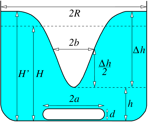
Figure 1: The most important optically observable parameters of the problem. Geometrical ones: $R$, the radius of the cylinder, $a$ and $d$ parameters of the stirrer, and $H$, the height of the still water. While stirring, further observable parameters are the displaced water height $H^{\prime}$, the distance $h$ between the funnel’s deepest point and the bottom of the container, the funnel’s depth and halfwidth $\Delta h=H^{\prime}-h$ and $b$, respectively.

The experiments were carried out with tap water in glass cylinders, in different combinations of radii $R$ and initial water heights $H$ as summarized in Table 1.

$R$ (cm)	$H$ (cm)
$3.8$	$12.0$
$6.5$	$16.8$
$10.5$	$24.8$
$22.4$	$27.1$

Table 1: The radii $R$ of the cylinders used and the heights $H$ to which water was filled up in each.

Two other relevant geometrical parameters are provided by the length $2a$ and the width $d$ of the magnetic stirrer bars (see Fig. 1). The different parameters of the bars used are summarized in Table 2.

When the rotation of the magnetic stirrer is switched on, the water column starts moving and after some time (which is on the order of minutes in our case) a statistically stationary flow sets in. Inherent fluctuations around the mean arise due to the periodic motion of the stirrer bar, the lack of a fixed axis of rotation, and turbulence. These are the physical reasons behind the relative errors of our measurements being on the order of $10$ percents. The most striking optically observable object is the funnel developing on the water surface. The height $H^{\prime}$ of the free surface at the perimeter and the characteristic sizes of the funnel, as defined in Fig. 1, can be easily measured (see Section IV).

IV Data acquisition

The rotation frequency $\Omega$ of the stirring bar in the container filled up with water was determined by means of a stroboscope whose frequency $f$ is adjustable in a broad range. At certain frequencies $f_{n}$ the bar appears to be at rest (see Fig. 2a). This happens if the bar rotates an integer multiple of a half rotation between two flashes, i.e., if

$$\frac{\Omega}{f_{n}}=n\pi.$$ (3)

The largest value of the $f_{n}$-s uniquely determines the bar’s rotation frequency as $\Omega=f_{1}\pi$. In order to reach a higher accuracy, we also determined the frequency $f_{1/2}$ when the bar rotates a right angle between two flashes. This case is designated by the appearance of a steady cross traced out by the bar on the bottom of the container (see Fig. 2b). The bar’s rotation frequency was determined as the average of the frequencies belonging to $f_{1}$ and $f_{1/2}$. The uncertainty in $f$ is $0.1$ Hz. In the range $(20,120)$ s^-1 of $\Omega$ investigated, this corresponds to a relative error of about $1$ percent, which is negligible compared to the other errors.

stirrer bar	$a$ (cm)	$d$ (cm)	symbol
i	$2.05$	$0.85$	$\bigtriangledown$
ii	$2.50$	$0.90$	$\Box$
iii	$4.00$	$1.00$	$\Diamond$

Table 2: Geometrical parameters of the stirrer bars and the symbols used to mark the corresponding measured data in Figs. 3 and 9.

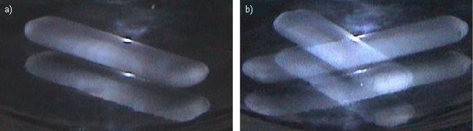
Figure 2: The apparent picture of the bar (along with its mirrored image by the bottom) at stroboscopic frequencies $f_{1}$ (a) and $f_{1/2}$ (b).

The funnel parameters were determined via direct optical observations. The water height $H^{\prime}$ in the statistically stationary state was measured by means of a ruler. The height of the funnel’s deepest point can be determined in a similar way or by using a horizontal laser sheet. From these two quantities, the funnel depth is simply $\Delta h=H^{\prime}-h$ (cf. Fig. 1). The halfwidth of the funnel was measured on the back side of the cylinder. The length obtained this way was corrected by taking into account the optical effect caused by the cylindrical lens formed by the water column to obtain the value $b$. Both the funnel depth and width are subjected to an error of about $10$ percents due to the fluctuations, c.f., Section III.

The particle image velocimetry (PIV) method was used to determine the velocity field in a plane defined by a horizontal laser sheet. From the position of fine tracer particles on two subsequent images taken with a time difference of about $10^{-2}$ s, the displacement and velocity of the particles can be determined.Dant We used a commercial PIV equipment (ILA GmbH, Germany) and determined the flow field in the largest container ($R=22.4$ cm) at an intermediate water height ($H=16.8$ cm) with stirrer bar ii (cf. Table 2) in different horizontal layers. The presence of the funnel and the strong downdraft make the PIV data unreliable in the middle of the container, within a region of radius of about $8$ cm.

Particle tracking enables us to study the central region of the flow. We used plastic beads (low density polyethylene) of diameter $\sim 1$ mm, which has a density of $\sim 0.92$ g/cm³. Despite being lighter than water, they sink below the funnel and often reach a dynamical steady state (for more detail see Subsection V.C). The approximate strength of the downwelling in the middle was estimated as the rising velocity of the beads in a water column at rest. From several measurements in a separate narrow glass cylinder we found this rising velocity to be $7$–$8$ cm/s, for all the beads used.

Spreading of dye can provide a qualitative picture about the flow. A particularly important region is that around the axis of the vortex, where this coloring technique reveals fine details (see Subsection V.D).

V Results

A. Frequency dependence of the funnel. The results of the optical observations of $16$ cases (different containers, water heights and stirring bars) each measured at several frequencies $\Omega$ are summarized in Fig. 3. While there is a clear frequency dependence on the funnel depth $\Delta h$, the halfwidth $b$ appears to be independent of $\Omega$ (see inset), in first approximation at least.

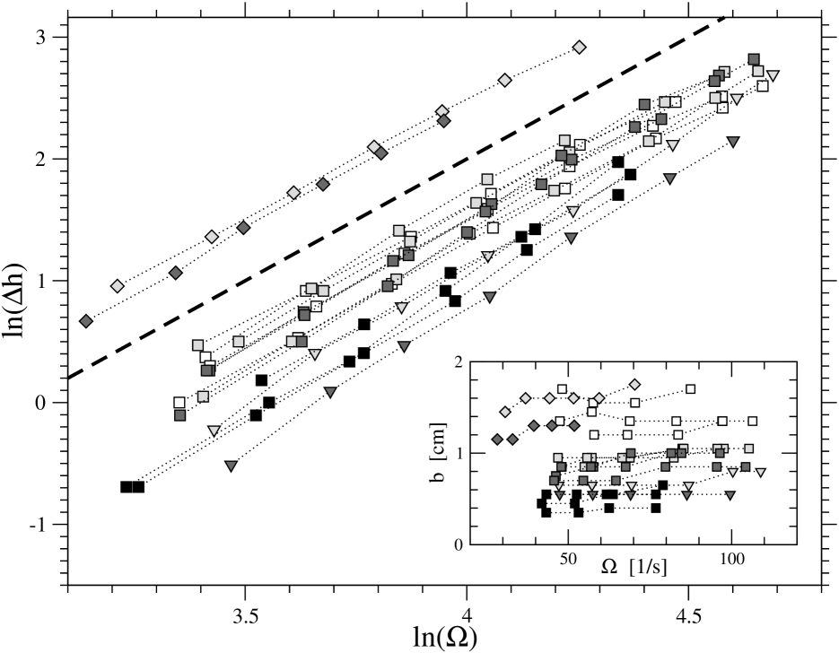
Figure 3: Funnel depth as a function of the rotation frequency in containers of different radii for different water heights and stirrer bars in double logarithmic representation. The slope of the dashed line is $2$. Inset: Funnel halfwidth as a function of the rotation frequency in different measurements. Different symbols mark different stirring bars (cf. Table 2), and the level of grayness increases with the radius of the container. Symbols are not distinguished according to water heights.

To extract the form of the frequency dependence, the funnel depth is plotted on log-log scale in Fig. 3. The straight lines clearly indicate a power-law dependence. The exponent is read off to be $2$:

$$\Delta h\sim\Omega^{2}.$$ (4)

One sees that the coefficient (not written out) depends much stronger on the stirring bar’s parameters $(a,d)$ than on the container’s geometry ($R,H$).

B. Velocity fields. First we present, in Fig. 4, the result of a typical PIV measurement in a horizontal plane. The arrows mark velocity vectors. Arrows around the vortex center are produced by algorithmic interpolation and cannot be considered therefore to be quantitatively reliable. The flow is not fully axially symmetric, small secondary vortices appear around the edges of the picture.

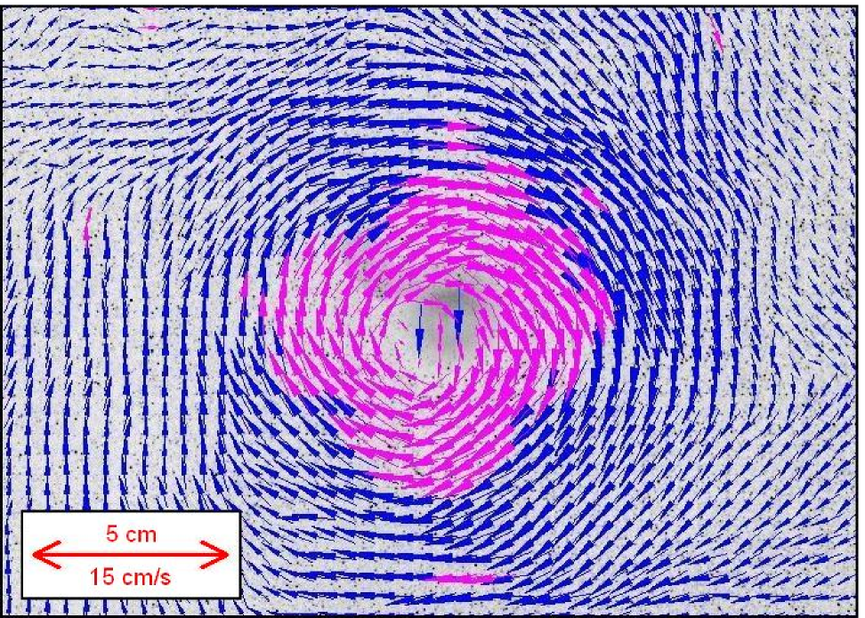
Figure 4: Detail of a PIV image at the height of $z=13$ cm taken at rotation frequency $\Omega=35.5$ s^-1 ($R=22.4$ cm, $H=16.8$ cm, $a=2.5$ cm, $d=0.9$ cm). The inset sets the length and velocity scales.

In order to understand the mean flow, we divided each PIV image into narrow concentric rings and evaluated the average tangential and radial velocity in each band. These values were further averaged over several images taken at different times in the same flow and at the same height. This way the effect of secondary vortices visible in Fig. 4 became averaged out. The procedure leads to a discrete representation of the functions $v_{t}(r)$ and $v_{r}(r)$. Both components appeared to be proportional to the frequency of the stirring bar, therefore we present in Fig. 5 the components already divided by $\Omega$. Since the results in the innermost region are not reliable, the components are displayed for distances $r>8$ cm only.

The measured tangential velocity data $v_{t}(r)$ can be approximated by a functional form $A/r$ satisfactorily. This behavior is demonstrated by plotting the rescaled quantity $v_{t}r/\Omega$ in Fig. 5, left column. (Note that the multiplication by $r$ magnifies the apparent error.) The coefficient $A$ is a weakly decreasing function of the depth. Nevertheless, the tangential flow matches that of an ideal vortex, as a first approximation. Accordingly, the vortex strength $C$ is proportional to the frequency, i.e.,

$$C=A\Omega$$ (5)

with a coefficient $A$ extracted from the data to be $A=0.9\pm 0.2$ cm².

In contrast to the tangential component, the radial component depends strongly on the height (Fig. 5, right column). In the upper layers there is an inflow ($v_{r}<0$) for $r>8$ cm at least, which decays towards zero as the height decreases. The level $z=4$ cm is dominated by outflow, but around $r=8$ cm a weak inflow survives.

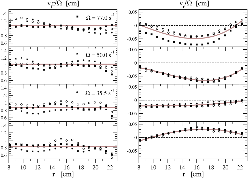
Figure 5: Rescaled tangential (left column) and radial (right column) velocity components $v_{t}r/\Omega$ and $v_{r}/\Omega$ for three values of $\Omega$ (see legends). PIV measurements carried out at different heights $z=$ 16, 13, 8, and 4 cm, from top to bottom. The horizontal lines on the left are fitted average values. The smooth curves on the right join the neighboring measured points to guide the eye.

The planar PIV algorithm does not provide any information on the vertical velocities. This component can, however, be determined from the continuity equation which takes the form LL ; Laut

$$\frac{\partial v_{z}}{\partial z}=-\frac{1}{r}\frac{\partial(rv_{r})}{\partial r}$$ (6)

in axisymmetric flows. We numerically integrated the left hand side to get an approximation for $v_{z}(r)$ from the radial component. This component turns out to be proportional to $\Omega$, too. The qualitative feature is that there is upwelling in the outermost $4-5$ cm and a slow downwelling in the intermediate region. The strong upwelling around the boundary of the container implies that there must be a strong downwelling in the very center, which, however, cannot be resolved by means of the PIV method.

C. Particle tracking. The strength of downwelling in the very center of the vortex can be estimated by means of monitoring plastic beads, lighter than water. They float on the surface but become eventually trapped by the funnel, on the surface of which they slide down and become advected downwards toward the bulk of the fluid (Fig. 6a). Along the axis of the vortex the particles reach a dynamical steady state (subjected, of course, to considerable fluctuations). This indicates that there is a strong downward jet in which the downward drag acting on the particle approximately compensates the upward resultant of gravity and buoyancy. As mentioned in Section IV, the asymptotic rising velocity of the beads is $7-8$ cm$/$s in a water of rest. Therefore we conclude that the strength of the downward jet is also $7-8$ cm$/$s.

A necessary condition for vertical stability is that the velocity of downwelling decreases when moving downwards along the axis. This occurs unavoidable in our case since the velocity should approach zero close to the lower bottom of the container. Experience shows that the average vertical position is shifted downwards when the frequency $\Omega$ is increased, since this makes the jet somewhat stronger.

Stability is maintained in the horizontal direction as well. This is due to the fact that in a rotating system an ‘anticentrifugal’ force acts on the bead since it is lighter than the surrounding fluid. Whenever the particle deviates from the axis, this force directs it backwards. This is accompanied by an immediate rising of the particle which indicates that the width of the strong downward jet is of the same order as the diameter of the particles. We conclude that this width is a few mm.

Due to the presence of all these effects and the permanent fluctuations of the flow, the overall motion of a particle is rather complex. After leaving the central jet, it starts rising but the ’anticentrifugal’ force pushes it back towards the center, at a larger height. Then it is captured by the jet and starts moving downwards again, and will leave the jet at another level than earlier. The bead remains within a cylindrical region around the vortex axis. We conclude that the particle motion is chaotic Ott (Fig. 6b). By tracking a single particle over a long period of time, a chaotic attractor is traced out (Fig. 6c).

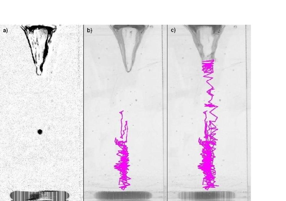
Figure 6: Particle tracking. a) A plastic bead lighter than water becomes washed downwards below the funnel. b) Path of the particle over $10$ s. c) Path of the particle over $20$ s.

D. Spreading of dye. When injecting dye into the water outside of the central region one observes a fast spreading. A drastically different behavior is found in the middle of the funnel. Very quickly, a cylindrical dye curtain develops around the vortex axis which remains observable over about a minute (Fig. 7). This can be seen at any value of the parameters ($R,H,a,d,\Omega$) investigated. The radius of the dye cylinder is on the order of the magnitude of the halfwidth $b$, it is about $1$ cm. It is remarkable that the wall of the cylindrical region containing the trapped beads (Fig. 6c) coincides with this dye curtain.

The existence of this long-lived dye curtain indicates that the radial velocity is approximately zero in a cylindrical annulus around the axis of rotation, the diameter of which is proportional to the width $d$ of the stirring bar. Since, while rotating, the bar continuously blocks the downward flow in a circle of diameter $d$, the suction is the strongest around the perimeter of this region. The downwelling has a maximum strength here, and it weakens inwards. In the very center, however, there is the central jet mentioned in Subsection V.C, therefore the existence of a local minimum is necessary. The injected dye accumulates along the surface in which the downward velocity takes its local minimum. Thus both inside and outside the cylinder surface the downward flow is stronger than on the surface itself, where injected dye accumulates. When injecting the dye somewhat off the cylinder one often observes more than one concentric curtains, as well (Fig. 7b). This indicates that there might be more local minima of the downward velocity in a region around the halfwidth of the funnel.

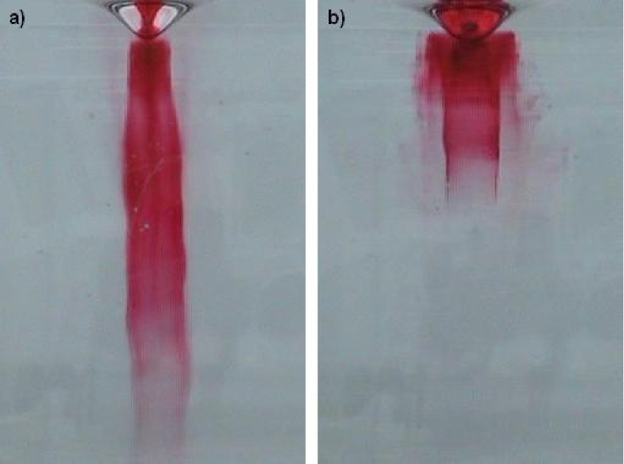
Figure 7: Dye pattern. (a) A stable cylindrical dye curtain (of lifetime over a minute) develops below the funnel. (b) Often sublayers can also be observed.

E. Qualitative picture. Based on the observations and the measurement of the velocity components, we obtain the following qualitative picture of the time averaged flow (Fig. 8). In a given vertical slice two flow cells are formed by the upwelling at the outer walls and the downwelling in the middle. In the three-dimensional space this corresponds to a torus flow whose central line lies in a horizontal plane, below the half of the water height. The flow along the central line has no radial and vertical component, a pure rotation takes place. The most striking feature is a strong downward jet in a very narrow filament on the axis of the vortex surrounded by a cylindrical region of weak downwelling.

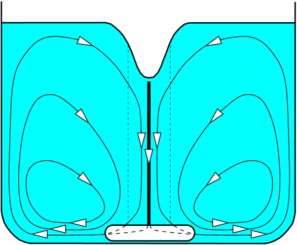
Figure 8: Pattern of the time averaged flow. The thin continuous lines represent streamlines, the bold line denotes the downward jet, and the dashed line represent the average location of dye curtains.

VI Quantitative results

A. Funnel depth. To obtain a simple expression for the funnel depth, we apply the method of dimensional analysis K ; X ; Y first, and a comparison with the measured data leads then to a particular form. As dimensionless measures of the viscous and gravitational effects in the rotating flow, a Reynolds and a Froude number is introduced as

$$Re=\frac{\Omega a^{2}}{\nu},\;\;\;\;\mbox{and}\;\;\;\;Fr=\frac{\Omega a}{(gR)^{1/2}}\frac{d}{a},$$ (7)

respectively. (The usual Froude number is multiplied by the factor $d/a$, in order to simplify the argumentation below.) Small values of them indicate strong viscous and gravitational effects. With our typical data ($\Omega=50$ s^-1, $R=10$ cm, $a=2.5$ cm, $d=1$ cm, $\nu=10^{-2}$ cm²s^-1) we obtain $Re=3\cdot 10^{4}$ and $Fr=0.5$. This indicates that gravity is essential, but viscosity is not so important for the overall flow. It is, however, obviously important on small scales, like e.g. in the center of the vortex.

The ratio $\Delta h/d$ must be a function of the dimensionless parameters, therefore we can write

$$\frac{\Delta h}{d}=f\!\left(Re,Fr,\frac{a}{d},\frac{a}{R},\frac{H}{R}\right)$$ (8)

with $f$ as an unknown function at this point. There might other dimensionless numbers also be present. One candidate would be a measure of the surface tension. This effect we estimated in control experiments with surfactants, and found a negligible influence with respect to our typical measurement error. Therefore, we do not include the corresponding dimensionless number into $f$.

Assuming that $f$ is linear in both $Re$ and $Fr$ we obtain

$$\frac{\Delta h}{d}=Re\,Fr\;\Phi\left(\frac{a}{d},\frac{a}{R},\frac{H}{R}\right).$$ (9)

This assumption is supported not only by (4), but by other observations as well: a careful investigation of the data shows that the funnel depth is proportional to $a^{2}$, and for sufficiently large radii ($R>0.4H$) it scales as $R^{-1/2}$. These observations imply that no $a/d$ and $a/R$-dependence remains in $\Phi$:

$$\frac{\Delta h}{d}=\frac{\Omega^{2}a^{2}d}{\nu(gR)^{1/2}}\;\Phi\!\left(\frac{H}{R}\right).$$ (10)

The form of the single-variable function $\Phi(x)$ can be estimated from a replotting of the data, as shown in Fig. 9. As the fitted smooth curve shows, a reasonable form of $\Phi$ is

$$\Phi\left(x\right)=\frac{1}{\alpha x+k}.$$ (11)

The best choice of the parameters is $\alpha=(0.58\pm 0.08)\cdot 10^{3}$, $k=(2.8\pm 0.2)\cdot 10^{3}$. The direct expression for the funnel depth is then

$$\Delta h=\frac{\Omega^{2}a^{2}d^{2}R^{1/2}}{\nu(\alpha H+kR)g^{1/2}}.$$ (12)

The result shows that the dependence on the water height is rather weak. This explains afterwards why it was worth defining the Froude number with $R$ in (7).

It is remarkable that such a simple formula can be found to the measured data with about $10$ percent accuracy.

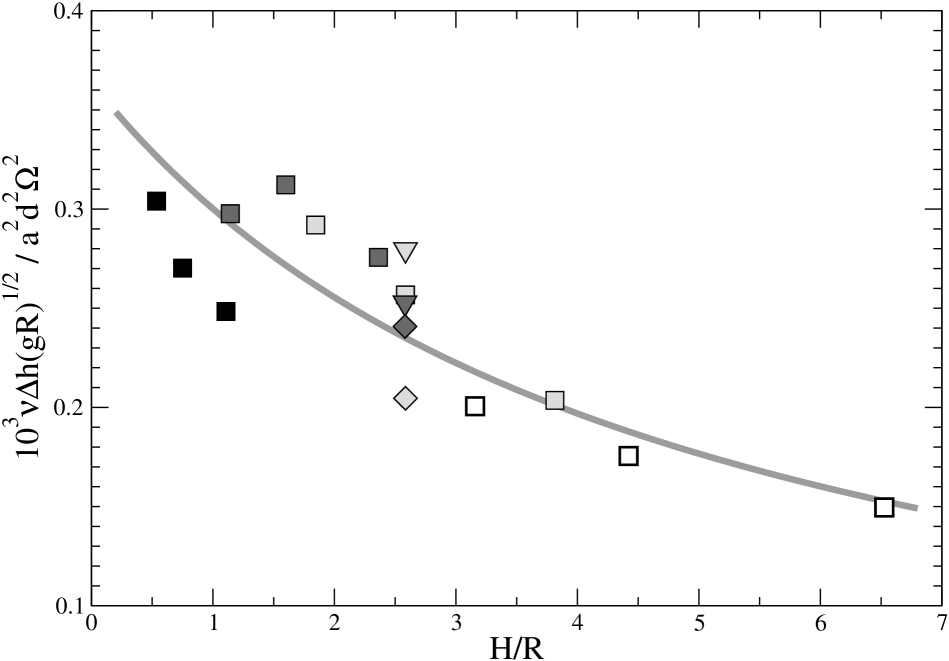
Figure 9: Determining the scaling function $\Phi(H/R)$ from the scaled measured $\Delta h/\Omega^{2}$ values averaged over different $\Omega$ values. The continuous line is a fitted hyperbola of the form of (11). The fact that several measured values belong to a given $H/R$ is due to the use of different stirrer bars. The use of symbols is similar as in Fig. 3.

B. Halfwidth. The halfwidth $b$ was found in Subsection V.A to be independent of $\Omega$. The ratio $b/d$ can therefore be written as

$$\frac{b}{d}=\frac{Fr}{Re}\,\Psi\!\left(\frac{a}{d},\frac{a}{R},\frac{H}{R}\right)=\frac{d\nu}{a^{2}(gR)^{1/2}}\Psi\!\left(\frac{a}{d},\frac{a}{R},\frac{H}{R}\right).$$ (13)

The data provide an essentially $H$-independent halfwidth which scales with $R^{-1/2}$. Therefore $\Psi$ must be independent of $H/R$ and $a/R$, i.e.,

$$\frac{b}{d}=\frac{d\nu}{a^{2}(gR)^{1/2}}\Psi\!\left(\frac{a}{d}\right).$$ (14)

Since the data show that $b$ is approximately linearly proportional to $a$, function $\Psi(x)$ should be cubic:

$$\Psi(x)=\beta x^{3},$$ (15)

and the best fit yields $\beta=(2.8\pm 0.8)10^{3}$. The direct expression for the halfwidth is then

$$b=\frac{\beta a\nu}{d(gR)^{1/2}}.$$ (16)

Note that this expression does not contain the water height at all.

C. Interpretation in terms of a Burgers vortex. The fact that the rotating motion in the magnetic stirrer flow is accompanied with an inflow and a downwelling resembles to the Burgers model treated in Section II. Equation (2) defines the plane $z=0$ as a plane without vertical velocity. Since far away from the center there is no downwelling on the free surface at height $H^{\prime}$, the $z=0$ level should be chosen as the topmost level of the rotated water. The vortex model obtained this way corresponds to the bulk of the investigated flow, far away from the external walls and the stirrer bar. It does not describe either the upwelling near the walls or the outdraft around the stirring bar.

The time independent nature of the axisymmetric mean flow implies that the pressure gradient compensates the centrifugal force and gravity in the radial and vertical direction:

$$\frac{\partial p}{\partial r}=\varrho\frac{v_{t}^{2}}{r},\;\;\;\;\frac{\partial p}{\partial z}=-\varrho g,$$ (17)

where $\varrho$ is the fluid density. On the fluid’s free surface at $z=\eta(r)<0$ $d\eta/dr=-({\partial p}/{\partial r})/({\partial p}/{\partial z})$. Consequently,

$$\frac{d\eta}{dr}=\frac{v_{t}^{2}}{rg}.$$ (18)

By inserting here the tangential velocity component from (2), the funnel depth can be obtained by integration:

$$\Delta h=\int_{0}^{R^{\prime}}\frac{C^{2}}{r^{3}g}\left(1-e^{-r^{2}/c^{2}}\right)^{2}dr.$$ (19)

Here $R^{\prime}\gg c$ is the radius within which the Burgers model is valid. Due to the exponential cut-off within the integrand the integral can well be approximated by taking $R^{\prime}=\infty$. We thus obtain

$$\Delta h=\ln{2}\frac{C^{2}}{c^{2}g}.$$ (20)

By equating this with the funnel depth expression (12) derived above, we recover relation $C=A\Omega$ found in Subsection V.B with a specific coefficient

$$A=a^{2}\left(\frac{\beta^{2}\nu}{\ln{2}(\alpha H+kR)(gR)^{1/2}}.\right)^{1/2}.$$ (21)

Similarly, from $c\approx b$ and the halfwidth expression (16) based on the measured data, we obtain

$$c=\frac{\beta a\nu}{d(gR)^{1/2}},$$ (22)

a relation already used in (21). Thus we are able to express both basic parameters, $C$ and $c$ of the Burgers model with the directly measurable parameters of the flow investigated.

VII Discussion

Here we compare the fluid dynamical properties of our experiment with that of other whirling systems: bathtub vortices, dust devils and tornadoes.

Detailed measurements of the velocities in these flows (see Refs. ABSRL, , Greeley, , and SHGLW, -SH, , respectively) indicate that, in spite of basic differences in the other components, the tangential component outside of the vortex core decays with distance $r$ as $C/r$, independently of height. The most dominant tangential component of all the flows is thus practically identical.

To estimate the degree of dynamical similarity in this component, we use another set of the dimensionless numbers:

$$Re^{\prime}=\frac{Uc}{\nu},\;\;\;\;Fr^{\prime}=\frac{U}{(gH)^{1/2}}.$$ (23)

Here $U$ represents the maximum velocity of the tangential flow component and $c$ denotes the radius of the vortex core.

flow	$U$ (m$/$s)	$H$ (m)	$c$ (m)	$Re^{\prime}$	$Fr^{\prime}$
stirrer	$0.5$	$0.2$	$10^{-2}$	$5\cdot 10^{3}$	$0.4$
bathtub	$0.4$	$0.1$	$2\cdot 10^{-4}$	$8\cdot 10^{2}$	$0.4$
dust devil	$25$	$10^{3}$	$50$	$8\cdot 10^{7}$	$0.25$
tornado	$70$	$10^{3}$	$200$	$10^{9}$	$0.7$

Table 3: Parameters and dimensionless numbers for the tangential velocity components of the flows compared.

The value of $U$ can be estimated in our case to be a few dm$/$s, for the estimate we take $50$ cm$/$s. The core radius and the height are $c\approx b\approx 1$ cm and $H\approx 20$ cm, respectively. The data for the other flows are taken from the literature and are summarized, along with the resulting dimensionless numbers in Table 3.

The Froude numbers are on the same order of magnitude but the Reynolds numbers are rather different. This shows that the role of viscosity is much stronger in small scale flows then in the atmosphere. Viscous flow is present in the vortex core, therefore the detailed flow patterns do not match there. The global flow is, however, in all cases practically that of an ideal fluid. Therefore we conclude that outside of the vortex core the tangential flows are dynamically similar, i.e. our experiment faithfully models all these whirling systems, an observation which can be utilized in undergraduate teaching.

Finally we mention that the analog of the dye curtain can be seen in tornadoes, typically in the vicinity of the bottom since it is the Earth surface which is the source of ‘dye’ (in the form of dust or debris). In some tornadoes this ‘dye’ curtain is clearly separated from the funnel (cf. e.g., http:$//$www.oklahomalightning.com).

This work was supported by the Hungarian Science Foundation (OTKA) under grants TS044839, T047233. IMJ thanks for a János Bolyai research scholarship of the Hungarian Academy of Sciences.

Appendix

Student Project 1. Explore the advection properties of small objects of different sizes, shapes and densities. Observe the rotation of elongated bodies (e.g., pieces of plastic straws) in the central jet. Their angular velocity monitors the local vorticity of the flow.

Student Project 2. As mentioned, one source of experimental errors is the oscillation of the stirrer bar. Try to eliminate this effect by slightly modifying the setup. Hint 1. Insert two magnetic stirrer bars in the opposite ends of a plastic tube with a hole between the two magnets. Use an external frame to fix a thin rod led through the hole to obtain a fixed axis of rotation. Hint 2. Use a narrow cylinder of nearly the same diameter as the length of the bar. Estimate the magnitude of the error and compare the parameters of the funnel in the modified and original setups.

References

- (1) L.D. Landau and E.M. Lifshitz, Fluid Dynamics (Pergamon Press, 1987)
- (2) H.J. Lugt, Vortex Flow in Nature and Technology (J. Wiley and Sons, 1983)
-
(3)
B. Lautrup, Continuum Physics: Exotic and Everyday
Phenomena in the Macroscopic World, Chapter 21: Whirls and Vortices,
http:www.cns.gatech.edu/PHYS-4421/Whirls.ps - (4) M. Raffael, C.E. Willert, J. Kompenhans: Particle Image Velocimetry: A Practical Guide (Spinger, Berlin, 1998)
- (5) E. Ott, Chaos in Dynamical Systems (Cambridge University Press, Cambridge, 1993, 2nd ed.: 2002)
- (6) P.K. Kundu, Fluid Dynamics, Academic Press, San Diego, 1990 (Chapter 8)
- (7) T.E. Faber, Fluid Dynamics for Physicists, Cambridge University Press, Cambridge, 1997 (Section 1.5)
- (8) Y. Nakayama and R.F. Boucher, Introduction to Fluid Mechanics, Arnold, London 1999 (Chapter 10)
- (9) A. Andersen, T. Bohr, B. Stenum, J.J. Rasmussen and B. Lautrup, Anatomy of a bathtub vortex, Phys. Rev. Lett. 91, 104502 (2003).
- (10) R. Greeley et al, Martian dust devils: laboratory simulation of particle threshold, J. Geophys. Res. 108, doi:10.12092002JE001987, (2003)
-
(11)
P. Sarkar, F. Haan, W. Gallus Jr., K. Le, J. Wurman: Velocity Measurements
in a Laboratory Tornado Simulator and their Comparison with Numerical and
Full-Scale Data
http:www.pwri.go.jp/eng/ujnr/joint/37/paper/42sarkar.pdf -
(12)
P. Sarkar, F. Haan Jr.: Next Generation Wind Tunnels for Simulation of
Straight-Line, Thunderstorm- and Tornado-Like Winds
http:www.pwri.go.jp/eng/ujnr/joint/34/paper/34sarkar.pdf