A study of the Navier-Stokes-$\alpha$ model for two-dimensional turbulence

E. Lunasin^A1, S. Kurien^A2, M. A. Taylor^A3 and E. S. Titi^A1,A4,A5

^A1Department of Mathematics, University of California, Irvine, CA, 92697, USA
^A2Theoretical Division, Los Alamos National Laboratory, Los Alamos, NM, 87544, USA
^A3Department of Exploratory Simulation Technologies, Sandia National Laboratories, Albuquerque, NM, 87185, USA
^A4Department of Computer Science and Applied Mathematics, Weizmann Institute of Science, Rehovot, 76100, Israel
^A5Department of Mechanical and Aerospace Engineering, University of California, Irvine, CA, 92697, USA

ABSTRACT. The Navier-Stokes-$\alpha$ sub-grid scale model of turbulence is a mollification of the Navier-Stokes equations in which the vorticity is advected and stretched by a smoothed velocity field. The smoothing is performed by filtering the velocity field over spatial scales of size smaller than $\alpha$. This is achieved by convolution with a kernel associated with the Green’s function of the Helmholtz operator scaled by a parameter $\alpha$. The statistical properties of the smoothed velocity field are expected to match those of Navier-Stokes turbulence for scales larger than $\alpha$, thus providing a more computable model for those scales. For wavenumbers $k$ such that $k\alpha>1$, corresponding to spatial scales smaller than $\alpha$, there are three candidate power laws for the energy spectrum, corresponding to three possible dynamical eddy turnover time scales in the model equations: one from the smoothed field, the second from the rough field and the third from a special combination of the two. Using two-dimensional turbulence as a test case, we measure the scaling of the spectra from high-resolution simulations of the Navier-Stokes-$\alpha$ model, in the limit as $\alpha{\rightarrow}\infty$. We show that the energy spectrum of the smoothed velocity field scales as $k^{-7}$ in the direct enstrophy cascade regime, consistent with dynamics dominated by the time scale of the rough velocity field. This result implies that the rough velocity field plays a crucial role in the development of the smoothed field even though the latter is the purported model for the Navier-Stokes turbulence. This effect must be taken into account when performing accurate simulations of the NS-$\alpha$ model.

Keywords: turbulence models; sub-grid scale models; large eddy simulations; two-dimensional Navier-Stokes-$\alpha$ model

2000 Mathematics Subject Classifications: 76F55; 76F65

1. Introduction

Let $v(x,t)$ denote the velocity field and $p(x,t)$ the pressure of a homogeneous incompressible fluid with constant density $\rho(x)=1$. The Navier-Stokes equations (NSE):

(1) $$\partial_{t}v-v\times(\nabla\times v) =-\nabla p+\nu\Delta v+f,$$

$$\nabla\cdot v =0,$$

$$v(x,0) =v^{in}(x),$$

govern the dynamics of such fluid flows, where the body force $f(x)$, the viscosity $\nu~{}>~{}0$, and the initial velocity field $v^{in}(x)$ are given. We supplement the system in (1) with periodic boundary conditions in a basic box $[0,L]^{n}$, where $n=2,\mbox{ or }3$. We assume here, $\int_{[0,L]^{n}}f(x)\;dx=\int_{[0,L]^{n}}v^{in}(x)\;dx=0$, which implies that $\int_{[0,L]^{n}}v(x,t)\;dx=0$ for all $t>0$. It is computationally prohibitively expensive to perform reliable direct numerical simulation (DNS) of the NSE for high Reynolds number flows, due to the wide range of scales of motion that need to be resolved. The use of numerical models allows researchers to simulate turbulent flows of interest using smaller computational resources. In this paper we study a particular sub-grid scale turbulence model known as the Navier-Stokes-$\alpha$ (NS-$\alpha$) model:

(2) $$\begin{aligned} \partial_{t}v-u\times\left(\nabla\times v\right)&=-\nabla p+\nu\Delta v+f\\ \nabla\cdot u=\nabla\cdot v&=0\\ v&=u-\alpha^{2}\Delta u.\end{aligned}$$

The system in (2) reduces to the Navier-Stokes system when $\alpha=0$, i.e. $u=v$. One can think of the parameter $\alpha$ as the length scale associated with the width of the filter which smooths $v$ to obtain $u$. The filter is associated with the Green’s function of the Helmholtz operator $(I-\alpha^{2}\Delta)$ (given in the third equation of (2)). When $\alpha>0$, notice that the nonlinear term $u\times(\nabla\times v)$ in (2) is milder than that in (1).

The inviscid and unforced version of the $\alpha$-model in (2) was derived in [19] based on the Hamilton variational principle subject to the incompressibility constraint $\mbox{div}\;v=0$. It is worth mentioning that the inviscid model, the so called Euler-$\alpha$ model, coincides with the inviscid second-grade non-Newtonian fluid model (see, e.g., [8, 9, 12]). By adding the viscous term $-\nu\Delta v$ and the forcing $f$ in an ad hoc fashion, the authors in [3, 4, 5] and [14] obtain the NS-$\alpha$ system (2) which they then named the viscous Camassa-Holm equations (VCHE), also known as the Lagrangian averaged Navier-Stokes-$\alpha$ model (LANS-$\alpha$). The LANS-$\alpha$ model is different from the viscous second-grade non-Newtonian visco-elastic fluid in that the viscous term in the former is $-\nu\Delta v$, distinguishable from $-\nu\Delta u$ in the latter. In references [3, 4, 5] it was found that the analytical steady state solutions for the 3d NS-$\alpha$ model compared well with averaged experimental data from turbulent flows in channels and pipes for wide range of Reynolds numbers. It was this fact which led the authors of [3, 4, 5] to suggest that the NS-$\alpha$ model be used as a closure model for the Reynolds averaged equations (RANS). It has since been discovered that there is in fact a whole family of ‘$\alpha$’- models which provide similar successful comparison with empirical data – among these are the Clark-$\alpha$ model [1, 10], the Leray-$\alpha$ model [7], the modified Leray-$\alpha$ model [20] and the simplified Bardina model [2, 24] (see also [27] for a family of similar models).

We assume periodic boundary conditions with basic box $[0,L]^{n}$, and denote the spatial Fourier coefficients of $u(x)$ and $v(x)$ by $\hat{u}(\xi)$ and $\hat{v}(\xi)$, respectively. Let $(\cdot,\cdot)$ denote the $L^{2}$-inner product and $|\cdot|$ denote the $L^{2}$-norm over the basic box $[0,L]^{n}$ (we also use $|\cdot|$ for the modulus of a vector). In the two-dimensional (2d) case we have two conserved quantities for the (inviscid and unforced) NS-$\alpha$ equations, namely the energy,

(3) $$E_{\alpha} = \sum_{|\xi|=1}^{\infty}E_{\alpha}(\xi)\mbox{\quad where, }$$

(4) $$E_{\alpha}(\xi) = \dfrac{1}{2}\left(\hat{v}(\xi)\cdot\hat{u}(\xi)\right)=\dfrac{1}{2}\left(|\hat{u}(\xi)|^{2}+\alpha^{2}|\xi|^{2}|\hat{u}(\xi)|^{2}\right)\;\;\;$$

and the enstrophy,

(5) $$\Omega_{\alpha} = \sum_{|\xi|=1}^{\infty}\Omega_{\alpha}(\xi)$$

(6) $$\mbox{where }\Omega_{\alpha}(\xi) = \frac{1}{2}|\hat{q}(\xi)|^{2}$$

(7) $$\mbox{~{}and the vorticity }\hat{q}(\xi) = (\widehat{\nabla\times v})(\xi).$$

The energy of the smoothed field $u$ is given by,

(8) $$E^{u} = \sum_{|\xi|=1}^{\infty}E^{u}(\xi)$$

(9) $$\mbox{where }E^{u}(\xi) = \frac{1}{2}|\hat{u}(\xi)|^{2},$$

and is not conserved in the inviscid and unforced equations.

For a wavenumber $k$, we define the component $u_{k}$ of a velocity field $u$ by

(10) $$u_{k}:=u_{k}(x)=\sum_{|\xi|=k}\hat{u}(\xi)e^{i\frac{2\pi}{L}\xi\cdot x},$$

and the component $u_{k^{\prime},k^{\prime\prime}}$ with a range of wavenumbers $[k^{\prime},k^{\prime\prime})$ by

(11) $$u_{k^{\prime},k^{\prime\prime}}:=u_{k^{\prime},k^{\prime\prime}}(x)=\sum_{k^{\prime}\leq k<k^{\prime\prime}}u_{k}.$$

Denote by $E_{\alpha}(k)$ the energy spectrum associated to

(12) $$\mathfrak{e}_{k}^{\alpha}=\dfrac{1}{2}\left\langle|u_{k,2k}|^{2}+\alpha^{2}|\nabla u_{k,2k}|^{2}\right\rangle,$$

which is the average energy per unit mass of eddies of linear size $l\in\biggl{(}\dfrac{1}{2k},\dfrac{1}{k}\biggr{]}$, then

(13) $$\mathfrak{e}_{k}^{\alpha}=\int_{k}^{2k}E_{\alpha}(\chi)\;d\chi.$$

Similarly, denote by $E^{u}(k)$ the energy spectrum associated to $\mathfrak{e}_{k}^{u}=\dfrac{1}{2}\left\langle|u_{k,2k}|^{2}\right\rangle$, that is,

(14) $$\mathfrak{e}_{k}^{u}=\int_{k}^{2k}E^{u}(\chi)\;d\chi.$$

In [15], it can be shown that $E^{u}(k)$ has the following remarkable property in three-dimensional (3d) viscous NS-$\alpha$ case,

(17) $$E^{u}(k)\sim\left\{\begin{array}[]{lll}k^{-5/3},&\mbox{when }&k\alpha\ll 1\\ k^{-\beta},&\mbox{when }&k\alpha\gg 1\end{array}\right.$$

where $\beta=3>5/3$, corresponds to a sharper roll-off than the NSE scaling of the energy power spectrum $k^{-5/3}$ for $k\alpha\gg 1$. Thus, $E^{u}(k)$ is offered as a model spectrum for the NSE for spatial scales of motion larger than $\alpha$. From the point of view of numerical simulation, the faster (compared to NSE) decay of $E^{u}(k)$ of NS-$\alpha$ for $k\alpha>1$, indicates suppression of scales smaller than $\alpha$ and in principle implies reduced resolution requirements for simulating a given flow. The scaling in the $k\alpha>1$ regime, that is, the exponent $\beta$, was determined in [14] using a time scale which depends solely on the smoothed velocity field. Later on, in [1, 7, 20], three possibilities for the exponent $\beta$ were derived since there are two velocities in the NS-$\alpha$ model. The three possibilities for the exponent $\beta$ depend on whether the turnover time scale of an eddy of size $k^{-1}$ is determined by $(k|u_{k}|)^{-1}$, $(k|v_{k}|)^{-1}$, or $(k\sqrt{(u_{k},v_{k})}\;)^{-1}$ (see e.g. [1, 20, 2, 15] and Section 2). Determining the actual scaling requires resolved numerical simulations. In the rest of the paper we will use the notation $E(k)$ and $E^{u}(k)$ interchangeably for finite $\alpha$ simulations when there is no ambiguity in meaning.

The 3d NS-$\alpha$ model was tested numerically in [6], for moderate Reynolds number in a simulation of size $256^{3}$, with periodic boundary conditions. It was observed that the large scale features of a turbulent flow were indeed captured and there was a rollover of the energy spectrum from $k^{-5/3}$ for $k\alpha\ll 1$ to something steeper for $k\alpha\gg 1$, although the scaling ranges were insufficient to enable extraction of the scaling exponent $\beta$ of (17) unambiguously. Other numerical tests of the NS-$\alpha$ model were performed in [17], [18], and [25], with similar results.

Our goal in this work is to measure the scaling of the energy spectrum of the NS-$\alpha$ in the regime $k\alpha\gg 1$ in the forward enstrophy cascade regime for 2d turbulence. Assuming the validity of the semi-rigorous arguments introduced in [15], we can then infer from our computations the timescale which governs the turnover of an eddy of size $1/k$. We choose to do this measurement for the 2d case with the expectation that discerning scaling ranges and exponents will be cheaper and more tenable in a 2d system than in a 3d system at the same grid-resolution. Nevertheless, we hope that the results in 2d will provide some insight into the turnover time of eddies of size $1/k$ for $k\alpha\gg 1$ in the 3d case.

In two-dimensional turbulence there are two inertial ranges, one for the inverse cascade of energy $E$ and the other for the direct cascade of enstrophy with corresponding scalings of the energy spectrum as follows [22]:

$$E(k)\sim\Big{\{}\begin{array}[]{lll}k^{-5/3},&\quad\mbox{where }&k\ll k_{f},~{}\mbox{inverse energy cascade regime}\\ k^{-3},&\quad\mbox{where }&k_{d}\gg k\gg k_{f},~{}\mbox{direct enstrophy cascade regime}\end{array}$$

where $k_{f}$ is the injection (forcing) wavenumber for both energy and enstrophy, and $k_{d}$ is the enstrophy dissipation wavenumber. The $k^{-3}$ scaling is thought to be accurate upto a log-correction [23]. In a NS-$\alpha$ model implementation, if we choose $\alpha$ smaller than the injection scale such that $k_{f}\alpha\ll 1$, we expect a modification of the scaling in the enstrophy cascade regime as follows

(22) $$E^{u}(k)\sim\left\{\begin{array}[]{lll}k^{-5/3},&\mbox{where }&k\ll k_{f},\\ k^{-3},&\mbox{where }&k_{f}\ll k\ll 1/\alpha,\\ k^{-\gamma},&\mbox{where }&1/\alpha\ll k\ll k_{d}\end{array}\right\}$$

where $\gamma>3$. For the 2d NS-$\alpha$, we show, using semi-rigorous arguments as in [1, 13, 20, 2, 15] that there are three possible scalings, $\gamma\in\{7,19/3,17/3\}$. We verify numerically which of these scalings actually emerges, and therefore deduce the eddy turnover time for the eddies of size smaller than the length scale $\alpha$.

As may be seen from Eqs. (22), for finite $\alpha$, there are three distinct scaling ranges for 2d NS-$\alpha$. Since we are primarily interested in the value of $\gamma$ we would like to maximize the range of scales over which $k^{-\gamma}$ scaling dominates. Therefore, we minimize the inverse cascade range of $k^{-5/3}$ scaling by forcing in the lowest modes. We also minimize the $k^{-3}$ scaling range by increasing $\alpha$ all the way to $\alpha\rightarrow\infty$. The latter limit is well-defined and yields what we will call the NS-$\infty$ equations (see, e.g. [21]):

(23) $$\begin{aligned} \partial_{t}v-u\times\nabla\times v&=-\nabla p+\nu\Delta v+f\\ \nabla\cdot u=\nabla\cdot v&=0\\ v&=-L^{2}\Delta u,\end{aligned}$$

where the forcing term was rescaled appropriately to avoid trivial dynamics. Assuming that the scaling of the spectrum as $\alpha\rightarrow\infty$ is identical to the scaling in the range $k\alpha\gg 1$, for finite (small) $\alpha$ and sufficiently long scaling ranges, we obtain the first resolved numerical calculation of the sub-$\alpha$ scales. The assumption is not unreasonable as nothing singular is expected to occur as $\alpha$ grows, other than the lengthening of the scaling range of interest. We remark, however, that one has to rescale the forcing appropriately in order to avoid trivial dynamics for large values of $\alpha$, and decaying turbulence at the limit when $\alpha{\rightarrow}\infty$.

The paper is organized as follows. In section 2 we summarize our analytical results. We show that the 2d NS-$\alpha$ model exhibits an inverse cascade of the energy $E_{\alpha}=\frac{1}{2}\int_{[0,L]^{2}}u(x)\cdot v(x)\;dx$ and a forward cascade of the enstrophy $\Omega_{\alpha}=\frac{1}{2}\int_{[0,L]^{2}}|q(x)|^{2}\;dx$, where $q(x)~{}=~{}\nabla~{}\times~{}v(x)$. Then, we show that in the forward enstrophy cascade regime, the energy of the smoothed velocity $E^{u}=\frac{1}{2}\int_{[0,L]^{2}}u(x)\cdot u(x)\;dx$ should follow the Kraichnan $k^{-3}$ power law for $k\alpha\ll 1$. For $k$ such that $k\alpha\gg 1$ and $k_{f}\ll k\ll k_{d}$, we will show how the three possible power laws, $k^{-17/3},k^{-19/3}$ and $k^{-7}$, arise.

In section 3 we present the details of our numerical scheme, data parameters and empirical justification for adopting a hypoviscousity sink term for the energy in the low modes. Our numerical calculations ranged in resolution from $256^{2}$ to $4096^{2}$. Our data show a convergence to $k^{-7}$ power law in the range $k\alpha\ll 1$ as $\alpha\rightarrow\infty$. This scaling allows us to conclude that the eddy turnover time in the enstrophy cascade region of the smoothed 2d NS-$\alpha$ energy spectrum is determined by the time scale which depends on the square of the unsmoothed velocity field, that is the variable $v$.

2. Statistical predictions for the NS-$\alpha$ model

2.1. Average transfer and cascade of energy and enstrophy for the 2d NS-$\alpha$ model

In two-dimensional turbulence, energy and enstrophy transfer behave as follows: in the wavenumber range below $k_{f}$, the energy and enstrophy go from higher modes to lower modes; in the wavenumber range above $k_{f}$, the energy and enstrophy go from low to high wavenumbers. In a certain wavenumber regime above $k_{f}$, there is much stronger direct transfer of enstrophy than energy, leading to what is called the direct enstrophy cascade. Similarly, in a certain range below $k_{f}$, there is a more dominant transfer of energy, leading to what is called the inverse energy cascade. For the 2d NS-$\alpha$ model we show that there is similar behaviour of transfer and cascade for its energy $E_{\alpha}$ and enstrophy $\Omega_{\alpha}$. We follow the techniques in [16] to arrive at this conclusion. Here we summarize our main results. The complete details can be found in the Appendix.

For $m\gg k_{f}$, let ${{\varepsilon}^{\alpha}_{m}}$ be the net amount of energy $E_{\alpha}$ (see (3)) transferred per unit time into the modes higher than or equal to $m$, and ${\eta^{\alpha}_{m}}$ be the net amount of enstrophy $\Omega_{\alpha}$ (see (5)) transferred per unit time into the modes higher than or equal to $m$. From the scale-by-scale evolution equation of energy $E_{\alpha}$ and enstrophy $\Omega_{\alpha}$ we get the following relationship between ${{\varepsilon}^{\alpha}_{m}}$ and ${\eta^{\alpha}_{m}}$

(24) $$\left\langle{{\varepsilon}^{\alpha}_{m}}\right\rangle\leq\dfrac{\left\langle{\eta^{\alpha}_{m}}\right\rangle}{m^{2}(1+\alpha^{2}m^{2})},$$

where $\left\langle\cdot\right\rangle$ denotes an ensemble average with respect to infinite time average measure (see Appendix). This result suggests that for large $m$, the average net of transfer of energy to high modes is significantly smaller than the corresponding transfer of enstrophy. This yields the characteristic direct enstrophy cascade.

The inverse energy cascade is expected to take place in the range below the $k_{f}$. Within this range, i.e. $m\ll k_{f}$, we obtain

(25) $$\left\langle-{\eta^{\alpha}_{m}}\right\rangle\leq m^{2}(1+\alpha^{2}m^{2})\left\langle-{{\varepsilon}^{\alpha}_{m}}\right\rangle,$$

that is, the (inverse) average net transfer of energy to lower modes is much stronger than the corresponding enstrophy transfer which yields the characteristic inverse energy cascade. This establishes the expected 2d NS-$\alpha$ cascades for energy $E_{\alpha}$ and enstrophy $\Omega_{\alpha}$.

2.2. NS-$\alpha$ model effects on the scaling of the energy spectrum in the enstrophy cascade regime

We next derive, using semi-rigorous arguments [13, 14], the expected scaling for the 2d NS-$\alpha$ energy spectrum. We start by splitting the flow into the three wavenumber ranges $[1,k),[k,2k),[2k,\infty)$. We assume $k_{f}<k$, where $k_{f}$ is the forcing wavenumber, since we are interested on the effects of the NS-$\alpha$ model in the enstrophy cascade regime. We decompose the $u$, $v$ and vorticity $q$ corresponding to the three wavenumber range, and for simplicity, we denote as follows:

$$u=u_{k}^{<}+u_{k,2k}+u_{2k}^{>}$$

$$v=v_{k}^{<}+v_{k,2k}+v_{2k}^{>}$$

$$q=q_{k}^{<}+q_{k,2k}+q_{2k}^{>},$$

where, $\phi_{l}^{<}=\phi_{1,l}$, $\phi_{l}^{>}=\phi_{l,\infty}$. We recall $\left(\cdot,\cdot\right)$ and $|\cdot|$ denote the $L^{2}$-inner product and $L^{2}$-norm respectively. The enstrophy balance equation for the NS-$\alpha$ model for an eddy of size $\sim k^{-1}$ is given by

(26) $$\hskip-20.2355pt\frac{1}{2}\;\frac{d}{dt}(q_{k,2k},q_{k,2k})+\nu(-\Delta q_{k,2k},q_{k,2k})=Z_{k}-Z_{2k},$$

where,

$$\begin{aligned} Z_{k}&:=-b(u_{k}^{<},q_{k}^{<},q_{k,2k}+q_{2k}^{>})+b(u_{k,2k}+u_{2k}^{>},q_{k,2k}+q_{2k}^{>},q_{k}^{<})\\ -Z_{2k}&:=-b(u_{2k}^{>},q_{2k}^{>},q_{k}^{<}+q_{k,2k})+b(u_{k}^{<}+u_{k,2k},q_{k}^{<}+q_{k,2k},q_{2k}^{>})\\ b(u,v,w)&:=\left(u\cdot\nabla v,w\right).\end{aligned}$$

$Z_{k}$ may be interpreted as the net amount of enstrophy per unit time that is transferred into wavenumbers larger than or equal to $k$. Similarly, $Z_{2k}$ represents the net amount of enstrophy per unit time that is transferred into wavenumbers larger than or equal to $2k$. Thus, $Z_{k}-Z_{2k}$ represents the net amount of enstrophy per unit time that is transferred into wavenumbers in the interval $[k,2k)$. Taking an ensemble average (with respect to infinite time average measure) of (26) we get

(27) $$\nu\left\langle(-\Delta q_{k,2k},q_{k,2k})\right\rangle=\left\langle Z_{k}\right\rangle-\left\langle Z_{2k}\right\rangle.$$

Using the definition of $E_{\alpha}(k)$ in (13), we can rewrite the averaged enstrophy transfer equation (27) as

$$\nu k^{5}(1+\alpha^{2}k^{2})E_{\alpha}(k)\sim\nu\int_{k}^{2k}k^{4}(1+\alpha^{2}k^{2})E_{\alpha}(k)dk\sim\left\langle Z_{k}\right\rangle-\left\langle Z_{2k}\right\rangle.$$

Thus, as long as $\nu k^{5}(1+\alpha^{2}k^{2})E_{\alpha}(k)\ll\left\langle Z_{k}\right\rangle$ (that is, $\left\langle Z_{2k}\right\rangle\approx\left\langle Z_{k}\right\rangle$, there is no leakage of enstrophy due to dissipation), the wavenumber $k$ belongs to the inertial range. Similar to the other $\alpha$-models, the correct averaged velocity of an eddy of length size $\sim 1/k$ is not known. That is, we do not know a priori in these models the exact eddy turnover time of an eddy of size $\sim 1/k$.

In the forward cascade inertial subrange, Kraichnan theory [22] postulates that the eddies of size larger than $1/k$ transfer their energy to eddies of size smaller than $1/(2k)$ in the time $\tau_{k}$ it takes to travel their length $\sim 1/k$. That is,

(28) $$\tau_{k}\sim\frac{1}{kU_{k}},$$

where $U_{k}$ is the average velocity of eddies of size $\sim 1/k$. Since there are two velocities in the NS-$\alpha$ model, there are three physically relevant possibilities for this average velocity, namely

$$\hskip-20.2355ptU_{k}^{0}=\left\langle\frac{1}{L^{2}}\int_{\Omega}|v_{k,2k}(x)|^{2}dx\right\rangle^{1/2}\sim\left(\int_{k}^{2k}(1+\alpha^{2}k^{2})E_{\alpha}(k)dk\right)^{1/2}\sim\left(k(1+\alpha^{2}k^{2})E_{\alpha}(k)\right)^{1/2},$$

$$\hskip-20.2355ptU_{k}^{1}=\left\langle\frac{1}{L^{2}}\int_{\Omega}u_{k,2k}(x)\cdot v_{k,2k}(x)dx\right\rangle^{1/2}\sim\left(\int_{k}^{2k}E_{\alpha}(k)dk\right)^{1/2}\sim\left(kE_{\alpha}(k)\right)^{1/2},$$

$$\hskip-20.2355ptU_{k}^{2}=\left\langle\frac{1}{L^{2}}\int_{\Omega}|u_{k,2k}(x)|^{2}dx\right\rangle^{1/2}\sim\left(\int_{k}^{2k}\frac{E_{\alpha}(k)}{(1+\alpha^{2}k^{2})}dk\right)^{1/2}\sim\left(\frac{kE_{\alpha}(k)}{1+\alpha^{2}k^{2}}\right)^{1/2}.$$

That is,

(29) $$U_{k}^{n}\sim\frac{(kE_{\alpha}(k))^{1/2}}{(1+\alpha^{2}k^{2})^{(n-1)/2}},~{}~{}(n=0,1,2).$$

We may therefore write the turnover time scale of an eddy of size $k^{-1}$ in (28) as

(30) $$\tau_{k}^{n}\sim\frac{1}{kU_{k}^{n}}=\frac{(1+\alpha^{2}k^{2})^{(n-1)/2}}{k^{3/2}(E_{\alpha}(k))^{1/2}},~{}~{}(n=0,1,2).$$

The enstrophy dissipation rate $\eta_{\alpha}$ which is a constant equal to the flux of enstrophy from wavenumber $k$ to $2k$ is given by

(31) $$\eta_{\alpha}\sim\frac{1}{\tau_{k}^{n}}\int_{k}^{2k}(1+\alpha^{2}k^{2})k^{2}E_{\alpha}(k)dk\sim\frac{k^{9/2}\left(E_{\alpha}(k)\right)^{3/2}}{(1+\alpha^{2}k^{2})^{(n-3)/2}},$$

and hence

$$E_{\alpha}(k)\sim\frac{\eta_{\alpha}^{2/3}(1+\alpha^{2}k^{2})^{(n-3)/3}}{k^{3}}.$$

Thus, the energy spectrum of the smoothed velocity $u$ is given by

(34) $$\hskip-20.2355ptE^{u}(k)\equiv\frac{E_{\alpha}(k)}{1+\alpha^{2}k^{2}}\sim\left\{\begin{array}[]{ll}\displaystyle{{\eta_{\alpha}^{2/3}}{k^{-3}},}&\mbox{when }k\alpha\ll 1\,,\\ \displaystyle{\frac{\eta_{\alpha}^{2/3}}{\alpha^{2(6-n)/3}}k^{-(21-2n)/3}},&\mbox{when }k\alpha\gg 1\,.\end{array}\right.$$

Therefore, depending on the average velocity of an eddy of size $k^{-1}$ for the NS-$\alpha$ model, we obtain three possible scalings of the energy spectrum, $k^{-(21-2n)/3}$, $(n=0,1,2)$ all of which decay faster than the Kraichnan $k^{-3}$ power law, in the subrange $k\alpha\gg 1$. We note that in the work of [26] the $k^{-17/3}$ power law was obtained using dimensional analysis, consistent with $n=2$ in our notation, using a time scale which depends solely on the smoothed velocity field. The actual power law was not determined at the time due to insufficient dynamic range of their simulations. Our simulations here show that the scaling is $k^{-7}$, which corresponds to $n=0$ in our notation.

3. Results

3.1. Details of the numerical simulation

The Navier-Stokes equations and the Navier-Stokes-$\alpha$ model equations with stochastic forcing were solved numerically in a periodic domain of length $L=1$ on each side. The wavenumbers $k$ are thus integer multiples of $2\pi$. A pseudospectral code was used with fourth-order Runge-Kutta time-integration. Simulations were carried out with resolutions ranging from $256^{2}$ to a maximum resolution of $4096^{2}$ on the Advanced Scientific Computing QSC machine at the Los Alamos National Laboratory. To maximize the enstrophy inertial subrange, the forcing is applied in the wavenumber shells $2<k<4$. We also add a hypoviscous term ($\mu\Delta^{-1}v$) which provides a sink in the low wavenumbers. Let $\mathcal{H}=1-\alpha^{2}\Delta$, then $v=\mathcal{H}u$. We simulate the following equation:

(35) $$\partial_{t}u-\mathcal{H}^{-1}(u\times(\nabla\times v))=-\nabla\pi+\mu(\Delta^{-1}u)+\nu\Delta u+f$$

where $\pi$ denotes the modified pressure and $\mu>0$ is a hypoviscosity coefficient. The equation in (35) is equivalent to

(36) $$\partial_{t}v-u\times\left(\nabla\times v\right) =-\nabla p+\mu(\Delta^{-1}v)+\nu\Delta v+\tilde{f},$$

where $\tilde{f}=\mathcal{H}(f)$ (compare with equation (2)). We demonstrate in the next section, that adding a hypoviscous term does not have a significant effect on our observed numerical results. We use no extra dissipation term in the small scales besides the regular dissipation in the Navier-Stokes or the Navier-Stokes-$\alpha$. Some relevant parameters and results of our simulation are presented in Table 1.

Table 1. Parameters of the simulations: number of grid points per side N, $\alpha$ in units of $\Delta x$, viscocity coefficient $\nu$, hypoviscosity coefficient $\mu$, maximum wavenumber $k_{max}=\dfrac{\sqrt{2}}{3}N$ , enstrophy dissipation scale $l_{\eta}=\left(\dfrac{\nu^{3}}{\eta_{\alpha}}\right)^{1/6}$, where $\eta_{\alpha}$ is the enstrophy dissipation rate.

N	$\alpha$	$\alpha/L$	$\nu$	$\mu$	$k_{max}l_{\eta}$
256	0	0	$1e^{-3}$	0	10
				5	10
				10	10
	2.04	0.008		0	10
				5	10
				10	10
	$\infty$	$\infty$		0	2
				5	2
				10	2
1024	0	0	$1e^{-4}$	15	12.5
	3.25	0.003			12.5
	15	0.015			12
	100	0.097			6
	$\infty$	$\infty$			2
2048	0	0	$5e^{-5}$	10	18
	6.5	0.003			18
	$\infty$	$\infty$			2
4096	0	0	$1e^{-5}$	10	15
	$\infty$	$\infty$			2

The $256^{2}$ simulations were performed to ascertain whether it was feasible to perform the computations in reasonable time without a low-wavenumber sink term, the hypoviscosity. The simulations of $1024^{2}$ and higher show the convergence of the scaling exponent of interest, namely the value of $\gamma$.

The condition for a resolved simulation is judged by the degree to which the enstrophy dissipation scale is resolved since the enstrophy cascade is expected to govern the dynamics in the range $k\gg k_{f}$. The enstrophy dissipation rate for NSE and NS-$\alpha$ are:

(37) $$\begin{aligned} \eta&=\eta_{\alpha}=\nu\langle|\nabla q|^{2}\rangle\end{aligned}$$

where $q=\nabla\times v$, and $v$ is respectively, either the NS velocity or the unfiltered velocity for the NS-$\alpha$. The enstrophy dissipation scale is then computed, following Kraichnan [22, 23], by dimensional analysis in a manner analogous to the way in which the Kolmogorov energy dissipation scale is calculated in 3d turbulence:

(38) $$l_{\eta_{[\alpha]}}=\left(\dfrac{\nu^{3}}{\eta_{[\alpha]}}\right)^{1/6}.$$

A resolved simulation has $k_{max}l_{\eta}>1$. In all our simulations, $k_{max}l_{\eta}\geq 2$, indicating well-resolved flow. Note, however, in table 1 that, keeping all other parameters fixed, increasing $\alpha$ decreases $k_{max}l_{\eta}$, indicating that as if the NS-$\alpha$ flow is less resolved, from the point of view of the enstrophy cascade, than the NSE for a given grid and viscosity. However, this observation is misleading since the computations for the NS-$\alpha$ were done with a rescaled forcing term with an amplitude growing indefinitely as $\alpha{\rightarrow}\infty$. Therefore, by increasing $\alpha$, the NS-$\alpha$ is forced more vigorously, and damped strongly. We discuss this further in section (3.4).

3.2. Dependence of scaling behaviour on hypoviscosity

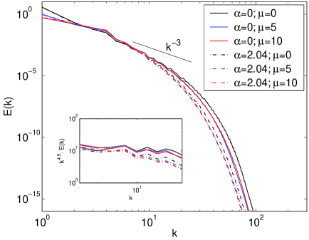
Figure 1. Energy spectra for a $256^{2}$ simulation with fixed viscosity and varying hypoviscosity coefficient $\mu$. The wavenumber $k$ is in multiples of $2\pi$. The solid lines are the DNS ($\alpha=0$) calculations of $E(k)$. The dotted lines are the NS-$\alpha$ model calculations of $E^{u}(k)$ for small $\alpha$. The behaviour of the spectra is largely independent of the magnitude of the hypoviscosity in the enstrophy cascade subrange ($6<k<15$). The inset shows the spectra compensated by $k^{4.5}$. The resolution of this simulation is far to small to observe the expected scaling exponent.

The hypoviscosity term in (36) provides a sink in the low wavenumbers for the energy. This allows the flow to reach statistical equilibrium in more reasonable computational time. However, since it is an ad hoc addition to the NSE or NS-$\alpha$ model, we need to ascertain whether it affects the behaviour in the range of scales of interest, namely the range $k>1/\alpha$.

In figure 1 we compare the energy spectra for $256^{2}$ run for DNS $(\alpha=0)$ and 2d NS-$\alpha$ with $\alpha=2.04$ (in units of $\Delta x$). The solid lines represent the DNS runs with varying hypoviscosity coefficient. In the inset, the compensated plots for the DNS show very little difference. The dotted lines correspond to the 2d NS-$\alpha$ runs with varying hypoviscosity coefficient. Again, as seen in the compensated plots in the inset, there is very little dependence on the hypoviscosity. These numerical results show that for a small to moderate hypoviscosity coefficient, the spectral slope in the enstrophy inertial range is not significantly affected by the addition of the hypoviscous term. Furthermore, as we see in Table 1 for the $256^{2}$ simulation, the enstrophy dissipation length scale $l_{\eta}$ is not affected by varying hypoviscosity coefficient.

From the above empirical observation, we conclude that, for the range of scales of interest, we can safely use a hypoviscous term and save significant computational time in our higher resolution runs.

3.3. Varying alpha; convergence to NS-$\infty$

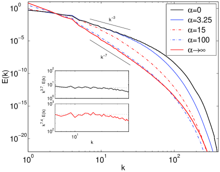
Figure 2. Energy spectra for $1024^{2}$ simulation. The black curve is the DNS ($\alpha=0$) which shows close to $k^{-3}$ scaling in the enstrophy cascade range $6<k<20$. The solid red curve is the $E^{u}(k)$ spectrum as $\alpha\rightarrow\infty$ which scales close to $k^{-7}$ in the enstrophy cascade range $6<k<25$. The energy spectra for intermediate values of $\alpha$ tend to the $\alpha\rightarrow\infty$ limit as $\alpha$ increases. The inset shows the DNS energy spectrum (black) compensated by $k^{3.7}$ and the $\alpha\rightarrow\infty$ energy spectrum (red) compensated by $k^{7.4}$

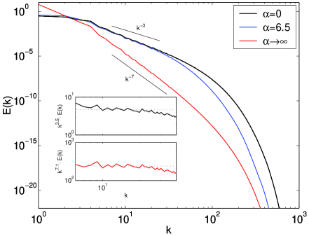
Figure 3. Energy spectra for $2048^{2}$ simulation. The wavenumber is in multiples of $2\pi$. The black curve is the energy spectrum of the DNS which shows close to $k^{-3}$ scaling in the enstrophy cascade range $6<k<35$. The solid red curve is the $E^{u}(k)$ spectrum as $\alpha\rightarrow\infty$ which scales approximately as $k^{-7.1}$ in the wavenumber region $6<k<25$. The inset shows the DNS energy spectrum (black) compensated by $k^{3.5}$ and the $\alpha\rightarrow\infty$ energy spectrum (red) compensated by $k^{7.1}$

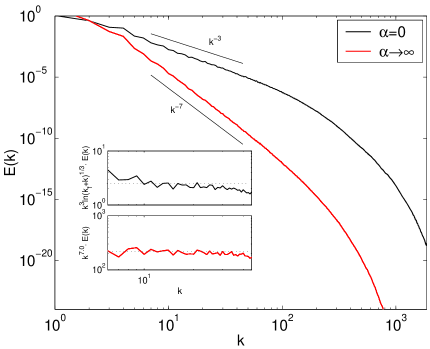
Figure 4. Energy spectra for $4096^{2}$ simulation. The black curve is the spectrum for the DNS, the red curve is the spectrum for $\alpha\rightarrow\infty$. The black curve in the inset corresponds to the NSE energy spectrum compensated by $k^{3}\ln(k_{f}+k)^{1/3}$ following [23]. The red curve in the inset is the energy spectrum $E^{u}(k)$ for NS-$\infty$ compensated by $k^{7}$. The region $6<k<40$ is flat indicating the nominal range over which the $k^{-7}$ scaling holds.

In this section we show the effect of varying the parameter $\alpha$. For a given grid, we fix the viscosity coefficient and vary $\alpha$ in order to measure the scaling exponent $\gamma$ of the energy spectrum in the enstrophy inertial subrange.

In figures 2, 3 and 4 we show the NSE spectrum $E(k)$ and the spectrum $E^{u}(k)$ from $1024^{2}$, $2048^{2}$ and $4096^{2}$ simulations, each with fixed viscosity and varying $\alpha$. As expected, the scaling ranges increase as the number of grid-points increase. In each figure the solid black line is the DNS spectrum $E(k)$, and approaches a scaling close to $k^{-3}$ as $N$ increases. In both Figs. 2 and 3 for $0<\alpha\leq 15$ (in units of $\Delta x$), we see the spectrum $E^{u}(k)$ peels away from the NSE spectrum ($\alpha=0$) near $k\alpha=1$ but displays no clear scaling behaviour for $k\alpha>1$ until $\alpha\geq 100$. To discern a clear power-law of the NS-$\alpha$ model spectrum, we consider the data from simulation of the NS-$\infty$ equations (23). This allows us to see the scaling of the NS-$\alpha$ model energy spectrum without contamination by finite-$\alpha$ or DNS for the NSE ($k^{-3}$) effects. At our maximum resolution of $4096^{2}$ in Fig. 4, as $\alpha{\rightarrow}\infty$ (solid red line), there is a clear convergence of the scaling to $k^{-7}$. Table 2 summarizes our findings for the scaling of the $E^{u}(k)$ spectrum as $\alpha{\rightarrow}\infty$ for each of our simulations.

Table 2. Convergence of $\alpha{\rightarrow}\infty$ scaling exponent $\gamma$ of $E^{u}(k)$ as the resolution is increased.

N	256	1024	2048	4096
$\gamma$	8.0	7.4	7.1	7.0

According to (34), the scaling $k^{-7}$ corresponds to an enstrophy turnover time scale determined by the velocity $v$. We conclude that the dynamics of the smoothed velocity field, which is the puported model for turbulence, is nevertheless still governed by the unfiltered velocity field.

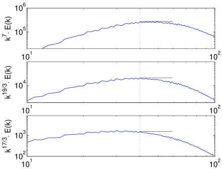
Figure 5. Compensated energy spectra for $2048^{2}$ simulation for $\alpha=6.5$ $(k_{\alpha}=39.75$; vertical dashed line). The energy spectrum is compensated by $k^{7},k^{19/3},\mbox{ and },k^{17/3}$ respectively. The region $39<k<70$ in the first subplot follows a flat regime which indicates the nominal range over which the $k^{-7}$ scaling holds.

In this analysis and conclusion, we have assumed that the scaling in the asymptotic limit $\alpha{\rightarrow}\infty$ would be identical to the scaling for $k\alpha>1$ for small $\alpha$. In Fig. 5 we demonstrate that this assumption is reasonable by showing that the scaling of the energy spectrum for small $\alpha=6.5$ is approaching close to $k^{-7}$ scaling for a small range of $k\alpha>1$. We are therefore reasonably convinced that going for the asymptotic limit is indeed giving us the correct scaling for finite (small) $\alpha$; the $\alpha{\rightarrow}\infty$ limit merely maximizes the range over which a clear scaling exponent can be measured at a given resolution.

3.4. NS-$\alpha$ model effects on the dissipation length scales of the flow

In Table 1, we observe that, keeping the viscosity, hypoviscosity and the resolution fixed, increasing $\alpha$ tends to decrease the enstrophy dissipation length-scale $l_{\eta}$ (see (38)). We also learned that the rate of dissipation of the energy $E^{u}$ is dictated by the eddy turnovertime of the unfiltered velocity field. In this section, we further explore the effects of the $\alpha$ parameter on the smallest scales of the flow. We recall that the NS-$\alpha$ computations were done with a rescaled forcing term, a fact which is important in the discussion to follow.

Table 3. Dissipation length scales when varying $\alpha$. N = resolution, $\alpha$, $\nu$ = visocisty coefficient, $\mu$ - hypoviscosity coefficient, $l_{\eta}$- enstrophy ($\Omega_{\alpha}$) dissipation length scale, $l_{\eta_{u}}$-smoothed enstrophy dissipation length scale

N	$\alpha$ (in units of $\Delta x$)	$\nu$	$\mu$	$l_{\eta}$	N	$\alpha^{\rm a}$	$\nu$	$\mu$	$l_{\eta_{u}}$
1024	0	$1e^{-4}$	15	.004133	1024	0	$1e^{-4}$	15	.004133
	3.25			.004099		3.25			.004490
	15			.003973		15			.005659
	100			.002165		100			.006827
	$\infty$			.000488		$\infty$			.006858

In the left panel of table 3, we present the enstrophy dissipation length scale $\l_{\eta}$ (see (38)) for the $1024^{2}$ simulation as $\alpha$ increases. This length scale, as we already know, gets smaller with increasing $\alpha$ value. A visual of this effect is given in Fig. 6, where we plot the isosurfaces of vorticity for increasing values of $\alpha$. Observe how the vorticity values grow while the vorticity structures become much finer as $\alpha$ increases.

By contrast, consider the right panel of table 3 where we present a “dissipation” length scale

(39) $$l_{\eta_{u}}=\left(\dfrac{\nu^{3}}{\eta_{u}}\right)^{1/6},$$

(40) $$\mbox{ where }\eta_{u}=\nu\left\langle|\nabla\omega|^{2}\right\rangle,$$

(41) $$\mbox{ and }\omega=\nabla\times u.$$

corresponding to a naively calculated length-scale for the smooth enstrophy $\Omega^{u}=|\nabla\times u|^{2}$. This length-scale grows as $\alpha$ increases. Corresponding to this we present in Fig. 7 the isosurfaces of $\nabla\times u$ for increasing values of $\alpha$. Note that in this case, the vorticity values diminish while the vorticity structures become increasingly smooth and diffuse.

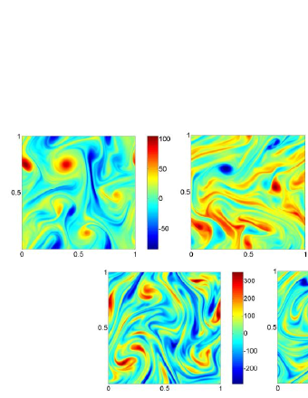
Figure 6. Isosurfaces of vorticity $\nabla\times v$ for the $1024^{2}$ simulation. $\alpha=0,3.25,15,100,\infty$, reading each row of figures from left to right. The vorticity field exhibits increasingly fine structures as $\alpha$ is increased.

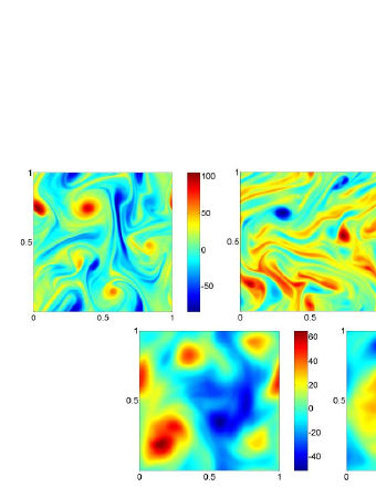
Figure 7. Isosurfaces of vorticity $\nabla\times u$ for the $1024^{2}$ simulation. $\alpha=0,3,25,15,100,\infty$, reading each row of figures from left to right. The structures become smoother with increasing $\alpha$.

Thus, on the one hand the smooth velocity field and its vorticity are consistent with reduced resolution requirements for the NS-$\alpha$ model; on the other, the behaviour of the conserved quantity for the (inviscid and unforced) NS-$\alpha$ model indicate a requirement for increased number of grid points, counter to what one would like to see in a sub-grid model. Note, however, that in order to avoid trivial dynamics as $\alpha$ increases, we have scaled the forcing term in the simulations of the NS-$\alpha$. That is, the computed Eq. (36) tends to the Eq. (23) as $\alpha\rightarrow\infty$. This was done so that we could conveniently study the case of large $\alpha$, thus extending the scaling range of interest. It could well be that for a detailed study of small-$\alpha$ with the forcing unscaled, the desired computational gains expected of a sub-grid model could be observed. However, our main goal in this study, the scaling exponent $\gamma$, could not be clearly obtained at achievable resolutions without going for the large-$\alpha$ limit. Thus, a straightforward comparison, for the purpose of checking the NS-$\alpha$ as a sub-grid model, is not clear. This implies that the implementation of the NS-$\alpha$ model as a turbulence model needs to be performed with some care.

Appendix A Average transfer and cascade of the energy $E_{\alpha}$ and enstrophy $\Omega_{\alpha}$ in the two-dimensional NS-$\alpha$ model

Here we will show analytically, the transfer and cascade of the energy in the two-dimensional NS-$\alpha$ model. Following the exposition as in [16], we will show that the conserved (in the absence of viscosity and forcing) energy $E_{\alpha}$ (3) and enstrophy $\Omega_{\alpha}$ (5) in the two-dimensional NS-$\alpha$ model have similar transfer and cascade behaviour as in the two-dimensional turbulence. We recall that we denote by $\phi_{l}^{<}=\phi_{1,l}$ and $\phi_{l}^{>}=\phi_{l,\infty}$

1. Average energy transfer
   We start by decomposing the velocity fields into two components: the large-scale component $u_{m}^{<}$ and $v_{m}^{<}$ containing eddies of size larger than $1/m$ and the small-scale component $u_{m}^{>}$ and $v_{m}^{>}$ containing eddies of size smaller than or equal to the lengthscale $1/m$. That is,

   $$\begin{aligned} u&=u_{m}^{<}+u_{m}^{>}\\ v&=v_{m}^{<}+v_{m}^{>}.\\ \end{aligned}$$

   For the forcing $f$, we assume it to be time independent and contains only finite number of modes, namely,

   $$f=f_{{{\underline{m}}},{{\overline{m}}}},\mbox{ where, }\;1<{{\underline{m}}}<{{\overline{m}}}<\infty.$$

   Here we will look at the two cases: $m\in(1,{{\underline{m}}})$ and $m\in({{\overline{m}}},\infty)$. We recall that $\left(\cdot,\cdot\right)$ and $|\cdot|$, denote the $L^{2}$-inner product and $L^{2}$-norm, respectively. From the above decomposition, we define the kinetic energy contained in the large and small eddies (respectively) as

   $$E^{<}_{\alpha}=\dfrac{1}{2}\left(u_{m}^{<},v_{m}^{<}\right)\;\;\mbox{ and }\;\;E^{>}_{\alpha}=\dfrac{1}{2}\left(u_{m}^{>},v_{m}^{>}\right).$$

   We are interested on how the energy $E_{\alpha}$ is transferred between large and small scales. Consider the case where $m>{{\overline{m}}}$ (i.e. beyond the injection of energy). Following the notation as in [14], let us denote by $\tilde{b}(u,v,w)=\left(-u\times(\nabla\times v),w\right)$. We write (2) in its functional differential form (see,e.g. [16, 28]),and apply the large and small scale decomposition to get the corresponding energy equations for the large and small scales

   (42) $$\begin{aligned} \dfrac{d}{dt}\left(v_{m}^{<},u_{m}^{<}\right)+\nu\left(v_{m}^{<},-\Delta u_{m}^{<}\right)+\tilde{b}(u_{m}^{<}+u_{m}^{>},v_{m}^{<}+v_{m}^{>},u_{m}^{<})&=\left(f,u_{m}^{<}\right)\\ \dfrac{d}{dt}\left(v_{m}^{>},u_{m}^{>}\right)+\nu\left(v_{m}^{>},-\Delta u_{m}^{>}\right)+\tilde{b}(u_{m}^{<}+u_{m}^{>},v_{m}^{<}+v_{m}^{>},u_{m}^{>})&=0.\end{aligned}$$

   Define

   (43) $$\begin{aligned} \Phi^{<}&:=-\tilde{b}(u_{m}^{>},v_{m}^{>},u_{m}^{<})+\tilde{b}(u_{m}^{<},v_{m}^{<},u_{m}^{>})\\ \Phi^{>}&:=\tilde{b}(u_{m}^{>},v_{m}^{>},u_{m}^{<})-\tilde{b}(u_{m}^{<},v_{m}^{<},u_{m}^{>})\\ \end{aligned}$$

   Notice that $\Phi^{>}+\Phi^{<}=0.$ We can rewrite the energy equations in the following form

   (44) $$\begin{aligned} \dfrac{d}{dt}E_{\alpha}^{<}+\nu\left(v_{m}^{<},-\Delta u_{m}^{<}\right)&=\Phi^{<}+\left(f,u_{m}^{<}\right)\\ \dfrac{d}{dt}E_{\alpha}^{>}+\nu\left(v_{m}^{>},-\Delta u_{m}^{>}\right)&=\Phi^{>}.\end{aligned}$$

   We can interpret the individual terms above as follows: $\left(f,u_{m}^{<}\right)$ - represents the energy flow injected into the large scales, by the forcing term. $\Phi^{<}$ - represents the net amount of energy per unit time that is transferred from small to large length scales. $\Phi^{>}$ - represents the net amount of energy per unit time that is transferred from large to small length scales. $-\tilde{b}(u_{m}^{<},v_{m}^{<},u_{m}^{>})$ - represents the energy flow induced in the high modes by inertial forces associated with lower modes.

   Let $\mathcal{F}$ be the set of all vector trigonometric polynomials with periodic domain $\Omega$. We then set $\mathcal{V}=\{\phi\in\mathcal{F}:\nabla\cdot\phi=0\mbox{ and }\int_{\Omega}\phi(x)\;dx=0\}$. We set $V$ to be the closure of $\mathcal{V}$ in the Sobolev space $H^{1}$. The solution operator $u(t)=S_{\alpha}(t)u_{0}$ of (2) defines a dynamical system on the phase space $V$. A generalized notion of infinite time averaging, as it was defined in [16], induces a probability invariant measure with respect to $S_{\alpha}(t)$. We denote this measure by $dP$, and the ensemble average with respect to this measure, will be denoted by

   (45) $$\left\langle\phi(\cdot)\right\rangle=\int_{V}\phi(w)dP(w).$$

   Thus, beyond the range where energy is injected, the average transfer of energy is into the higher modes, that is

   (46) $$\left\langle\Phi^{>}\right\rangle=\nu\left\langle v_{m}^{>},-\Delta u_{m}^{>}\right\rangle\geq 0.$$

   Now consider modes that are below the injection of energy. For that purpose, assume ${{\underline{m}}}>1$ and consider $m$ such that $1<m<{{\underline{m}}}$. The NS-$\alpha$ equation (2) can be decomposed as follows:

   (47) $$\begin{aligned} \dfrac{d}{dt}\left(v_{m}^{<},u_{m}^{<}\right)+\nu\left(v_{m}^{<},-\Delta u_{m}^{<}\right)+\tilde{b}(u_{m}^{<}+u_{m}^{>},v_{m}^{<}+v_{m}^{>},u_{m}^{<})&=0\\ \dfrac{d}{dt}\left(v_{m}^{>},u_{m}^{>}\right)+\nu\left(v_{m}^{>},-\Delta u_{m}^{>}\right)+\tilde{b}(u_{m}^{<}+u_{m}^{>},v_{m}^{<}+v_{m}^{>},u_{m}^{>})&=\left(f,u_{m}^{>}\right).\end{aligned}$$

   The associated energy equation for the lower modes reads:

   $$\dfrac{d}{dt}E_{<}^{\alpha}+\nu\left(v_{m}^{<},-\Delta u_{m}^{<}\right)=\Phi^{<}.$$

   We then take the ensemble average to get

   (48) $$\left\langle\Phi^{<}\right\rangle=\nu\left\langle v_{m}^{<},-\Delta u_{m}^{<}\right\rangle\geq 0.$$

   That is, for wavenumber regime below the injection of energy the average transfer of energy is from high wavenumbers to lower wavenumbers.
   

2. Average enstrophy transfer
   Next we consider the details of the transfer of enstrophy. Again, we assume $f$ is time independent and contains only a finite number of modes. Here, we do a slightly different exposition as in [16]. We take the curl of the momentum equation and using the incompressibility condition and the vector identity,

   (49) $$\nabla\times(a\times b)=a(\nabla\cdot b)-b(\nabla\cdot a)-(a\cdot\nabla)b+(b\cdot\nabla)a,$$

   we get the vorticity formulation for the 2d NS-$\alpha$ equation:

   (50) $$\partial_{t}q-\nu\Delta q+u\cdot\nabla q=\nabla\times f$$

   where, $q=\nabla\times v$ and we recall that $v=u-\alpha^{2}\Delta u$. We split the flow into two components $u=u_{m}^{<}+u_{m}^{>}\mbox{ and }q=q_{m}^{<}+q_{m}^{>}$.

   The amount of enstrophy contained in the large and small eddies are given, respectively, by

   (51) $$\begin{aligned} \Omega_{\alpha}^{<}&=|\nabla\times v_{m}^{<}|^{2}\\ \Omega_{\alpha}^{>}&=|\nabla\times v_{m}^{>}|^{2}.\end{aligned}$$

   We would like to show how the enstrophy is transferred between the large and small scales. First consider the case $m>{{\overline{m}}}$ (i.e. beyond the injection of energy). Following the notation as in the NSE [16], we denote by $b(u,v,w)=\left(u\cdot\nabla v,w\right)$. We write the evolution of the enstrophy governing the large and small scales:

   (52) $$\begin{aligned} \dfrac{d}{dt}\left(q_{m}^{<},q_{m}^{<}\right)+\nu\left(q_{m}^{<},-\Delta q_{m}^{<}\right)+b(u_{m}^{<}+u_{m}^{>},q_{m}^{<}+q_{m}^{>},q_{m}^{<})&=\left(\nabla\times f,q_{m}^{<}\right)\\ \dfrac{d}{dt}\left(q_{m}^{>},q_{m}^{>}\right)+\nu\left(q_{m}^{>},-\Delta q_{m}^{>}\right)+b(u_{m}^{<}+u_{m}^{>},q_{m}^{<}+q_{m}^{>},q_{m}^{>})&=0.\end{aligned}$$

   where, we denote by

   (53) $$\begin{aligned} \Psi^{<}&:=-b(u_{m}^{<}+u_{m}^{>},q_{m}^{<}+q_{m}^{>},q_{m}^{<})=-b(u_{m}^{<},q_{m}^{<},q_{m}^{>})+b(u_{m}^{>},q_{m}^{>},q_{m}^{<})\\ \Psi^{>}&:=-b(u_{m}^{<}+u_{m}^{>},q_{m}^{<}+q_{m}^{>},q_{m}^{>})=b(u_{m}^{<},q_{m}^{<},q_{m}^{>})-b(u_{m}^{>},q_{m}^{>},q_{m}^{<})\end{aligned}$$

   $\Psi^{<}$ - is the net amount of enstrophy transferred into low modes and $\Psi^{>}$ - is the net amount of enstrophy transferred into high modes. Note that for almost every $t$, $\Psi^{<}+\Psi^{>}=0$. From this we can rewrite the enstrophy equations above in the following form

   (54) $$\begin{aligned} \dfrac{1}{2}\dfrac{d}{dt}|q_{m}^{<}|^{2}+\nu|\nabla q_{m}^{<}|^{2}&=\Psi^{<}+\left(\nabla\times f,q_{m}^{<}\right)\\ \dfrac{1}{2}\dfrac{d}{dt}|q_{m}^{>}|^{2}+\nu|\nabla q_{m}^{>}|^{2}&=\Psi^{>}.\end{aligned}$$

   Taking the ensemble average (with respect to the infinite time averaging measure $dP$) of the equation for enstrophy associated with the low modes, we get

   (55) $$\left\langle\Psi^{>}\right\rangle=\nu\left\langle|\nabla q_{m}^{>}|^{2}\right\rangle\geq 0.$$

   This implies that, beyond the injection of energy, the average transfer of enstrophy is from low modes into higher modes. Next we consider the modes below the injection of energy. Assume $1<m<{{\underline{m}}}$, we get

   (56) $$\begin{aligned} \dfrac{d}{dt}\left(q_{m}^{<},q_{m}^{<}\right)+\nu\left(q_{m}^{<},-\Delta q_{m}^{<}\right)+b(u_{m}^{<}+u_{m}^{>},q_{m}^{<}+q_{m}^{>},q_{m}^{<})&=0\\ \dfrac{d}{dt}\left(q_{m}^{>},q_{m}^{>}\right)+\nu\left(q_{m}^{>},-\Delta q_{m}^{>}\right)+b(u_{m}^{<}+u_{m}^{>},q_{m}^{<}+q_{m}^{>},q_{m}^{>})&=\left(\nabla\times f,q_{m}^{>}\right).\end{aligned}$$

   We take the ensemble average of enstrophy equation associated with the low modes to get

   $$\left\langle\Psi^{<}\right\rangle=-\left\langle\Psi^{>}\right\rangle=\nu|\nabla q_{m}^{<}|^{2}\geq 0,$$

   that is, the average net transfer of enstrophy is from high modes to lower modes for wavenumber regime below the injection of energy.
   

3. Direct enstrophy cascade and inverse energy cascade
   In (i) and (ii) we have seen that in the range above the injection of energy both the energy and enstrophy is transferred from low to higher wavenumbers. On the wavenumbers regime below the injection of energy, both the energy and enstrophy are transferred from high to lower wavenumbers. Here we will show that, in the wavenumbers regime above the injection of energy, there is a much stronger transfer of enstrophy leading to what is called direct enstrophy cascade . On the other hand, in the wavenumbers regime below the injection of energy, the energy transfer is much stronger than the enstrophy transfer leading to what is known as the inverse cascade of energy.

   We split the flow into three parts assuming the same form restriction on the forcing as above. Consider $m^{\prime\prime}\geq m^{\prime}\geq{{\overline{m}}}$. Let $u=u_{m^{\prime}}^{<}+u_{m^{\prime},m^{\prime\prime}}+u_{m^{\prime\prime}}^{>}$ and $q=q_{m^{\prime}}^{<}+q_{m^{\prime},m^{\prime\prime}}+q_{m^{\prime\prime}}^{>}$. The vorticity field associated with the wavenumbers between $m^{\prime}$ and $m^{\prime\prime}$ is

   $$\dfrac{d}{dt}q_{m^{\prime},m^{\prime\prime}}-\nu\Delta q_{m^{\prime},m^{\prime\prime}}+B(u_{m^{\prime}}^{<}+u_{m^{\prime},m^{\prime\prime}}+u_{m^{\prime\prime}}^{>},q_{m^{\prime}}^{<}+q_{m^{\prime},m^{\prime\prime}}+q_{m^{\prime\prime}}^{>})=0$$

   where we denote by $B(v,w):=(v\cdot\nabla)w$. The evolution equation for the enstrophy associated with the modes between $m^{\prime}$ and $m^{\prime\prime}$ is given by

   $$\begin{aligned} \dfrac{1}{2}\dfrac{d}{dt}|q_{m^{\prime},m^{\prime\prime}}|^{2}&+\nu|\nabla q_{m^{\prime},m^{\prime\prime}}|^{2}\\ &=-b(u_{m^{\prime}}^{<}+u_{m^{\prime},m^{\prime\prime}}+u_{m^{\prime\prime}}^{>},q_{m^{\prime}}^{<}+q_{m^{\prime},m^{\prime\prime}}+q_{m^{\prime\prime}}^{>},q_{m^{\prime},m^{\prime\prime}}),\end{aligned}$$

   where, $b(u,v,w):=((u\cdot\nabla)v,w)$. One can compute by using the bilinear properties of $b$ (see, e.g. [11, 28, 16]) that,

   (57) $$\begin{aligned} -b(u_{m^{\prime}}^{<}+u_{m^{\prime},m^{\prime\prime}}+u_{m^{\prime\prime}}^{>},q_{m^{\prime}}^{<}+q_{m^{\prime},m^{\prime\prime}}+q_{m^{\prime\prime}}^{>},q_{k})&=\eta_{m^{\prime}}^{\alpha}-\eta_{m^{\prime\prime}}^{\alpha}\end{aligned}$$

   where,
   $\eta^{\alpha}_{m^{\prime}}$ - is the net amount of enstrophy transferred per unit time into the modes higher than or equal to $m^{\prime}$ and $\eta^{\alpha}_{m^{\prime\prime}}$ - is the net amount of enstrophy transferred per unit time into the modes higher than or equal to $m^{\prime\prime}$, and given by

   $$\begin{aligned} \eta^{\alpha}_{m^{\prime}}&=-b(u_{m^{\prime}}^{<},q_{m^{\prime}}^{<},q_{m^{\prime},m^{\prime\prime}}+q_{m^{\prime\prime}}^{>})+b(u_{m^{\prime},m^{\prime\prime}}+u_{m^{\prime\prime}}^{>},q_{m^{\prime},m^{\prime\prime}}+q_{m^{\prime\prime}}^{>},q_{m^{\prime}}^{<})\\ -\eta^{\alpha}_{m^{\prime\prime}}&=-b(u_{m^{\prime\prime}}^{>},q_{m^{\prime\prime}}^{>},q_{m^{\prime}}^{<}+q_{m^{\prime},m^{\prime\prime}})+b(u_{m^{\prime}}^{<}+u_{m^{\prime},m^{\prime\prime}},q_{m^{\prime}}^{<}+q_{m^{\prime},m^{\prime\prime}},q_{m^{\prime}}^{>}).\end{aligned}$$

   In explicit form we have

   (58) $$\dfrac{1}{2}\dfrac{d}{dt}|q_{m^{\prime},m^{\prime\prime}}|^{2}+\nu|\nabla q_{m^{\prime},m^{\prime\prime}}|^{2}=\eta^{\alpha}_{m^{\prime}}-\eta^{\alpha}_{m^{\prime\prime}}.$$

   Take the ensemble average of (58), we get

   $$\left\langle\eta^{\alpha}_{m^{\prime\prime}}\right\rangle=\left\langle\eta^{\alpha}_{m^{\prime}}\right\rangle-\nu\left\langle|\nabla q_{m^{\prime},m^{\prime\prime}}|^{2}\right\rangle.$$

   That is, the average net transfer of enstrophy into the modes higher than $m^{\prime\prime}$ is equal to the average net transfer of enstrophy into the modes higher than or equal to $m^{\prime}$ minus the enstrophy lost due to viscous dissipation within the range $[m^{\prime},m^{\prime\prime}]$. In $[m^{\prime},m^{\prime\prime}]$, it is assumed that the viscous dissipation is negligible and the enstrophy is simply transferred to smaller and smaller eddies. This occurs whenever

   (59) $$\left\langle\eta^{\alpha}_{m^{\prime\prime}}\right\rangle\geq\left\langle\eta^{\alpha}_{m^{\prime}}\right\rangle\gg\nu\left\langle|\nabla q_{m^{\prime},m^{\prime\prime}}|^{2}\right\rangle$$

   The range of wavenumbers $k>{{\overline{m}}}$ up to where (59) holds is called the enstrophy inertial subrange. Now within this range there is still an average net transfer of energy to higher modes. Denote by $\left\langle{{\varepsilon}^{\alpha}_{m}}\right\rangle:=\left\langle\Phi^{>}\right\rangle$ and $\left\langle{\eta^{\alpha}_{m}}\right\rangle:=\left\langle\Psi^{>}\right\rangle$. From (46) and (55)

   $$\dfrac{1}{\nu}\left\langle{{\varepsilon}^{\alpha}_{m}}\right\rangle\leq\dfrac{\left\langle|q_{m,\infty}|^{2}\right\rangle}{1+\alpha^{2}m^{2}}\leq\dfrac{\left\langle|\nabla q_{m,\infty}|^{2}\right\rangle}{m^{2}(1+\alpha^{2}m^{2})}=\dfrac{1}{\nu}\dfrac{\left\langle{\eta^{\alpha}_{m}}\right\rangle}{m^{2}(1+\alpha^{2}m^{2})}$$

   Hence,

   (60) $$\left\langle{{\varepsilon}^{\alpha}_{m}}\right\rangle\leq\dfrac{\left\langle{\eta^{\alpha}_{m}}\right\rangle}{m^{2}(1+\alpha^{2}m^{2})}.$$

   This result suggests that for large $m$, in particular, $k_{f}<m<k_{d}$, where $k_{d}$ is the dissipation wavenumber, the average net of transfer of energy to high modes is significantly smaller than the corresponding transfer of enstrophy. This yields the characteristic direct enstrophy cascade in this range.

   The inverse energy cascade takes place in the range below the injection of energy. Consider $1<m^{\prime}<m^{\prime\prime}<{{\underline{m}}}$. We follow the same steps as above. We decompose the flow into three components $u=u_{m^{\prime}}^{<}+u_{m^{\prime},m^{\prime\prime}}+u_{m^{\prime\prime}}^{>}$ and proceeding as before we obtain

   (61) $$\left\langle{\varepsilon}^{\alpha}_{m^{\prime\prime}}\right\rangle=\left\langle{\varepsilon}^{\alpha}_{m^{\prime}}\right\rangle+\nu\left\langle\left(v_{m^{\prime}m^{\prime\prime}},-\Delta u_{m^{\prime},m^{\prime\prime}}\right)\right\rangle$$

   As we have seen in (i) we have in this case the inverse transfer of energy

   $$\left\langle{\varepsilon}^{\alpha}_{m^{\prime\prime}}\right\rangle\leq 0\;\mbox{ and }\;\left\langle{\varepsilon}^{\alpha}_{m^{\prime}}\right\rangle\leq 0$$

   Therefore, as long as

   (62) $$\left\langle{\varepsilon}^{\alpha}_{m^{\prime\prime}}\right\rangle\lesssim\left\langle{\varepsilon}^{\alpha}_{m^{\prime}}\right\rangle\ll\nu\left\langle v_{m^{\prime},m^{\prime\prime}},-\Delta u_{m^{\prime},m^{\prime\prime}}\right\rangle$$

   we have inverse cascade. Now within the range corresponding to energy cascade (below injection of the force $f$) both the energy and enstrophy are transferred to lower modes

   $$\begin{aligned} \left\langle-{{\varepsilon}^{\alpha}_{m}}\right\rangle&=\nu\left\langle\left(\nabla v_{1,m},\nabla u_{1,m}\right)\right\rangle=\nu\left\langle|\nabla u_{1,m}|^{2}+\alpha^{2}|\Delta u_{1,m}|^{2}\right\rangle\geq 0\\ \left\langle-{\eta^{\alpha}_{m}}\right\rangle&=\nu\left\langle|\nabla q_{1,m}|^{2}\right\rangle\geq 0\end{aligned}$$

   Since $u_{1,m}$ contains only modes smaller than $m$, we therefore have

   (63) $$|\nabla q_{1,m}|^{2}\leq m^{2}(1+\alpha^{2}m^{2})\left(\nabla v_{1,m},\nabla u_{1,m}\right)$$

   which implies

   (64) $$\left\langle-{\eta^{\alpha}_{m}}\right\rangle\leq m^{2}(1+\alpha^{2}m^{2})\left\langle-{{\varepsilon}^{\alpha}_{m}}\right\rangle$$

   that is, in the wavenumber regime below the injection of energy, the (inverse) average net transfer of energy to lower modes is much stronger than the corresponding enstrophy transfer which yields the characteristic inverse energy cascade.

References

• [1] C. Cao, D. Holm and E.S. Titi, On the Clark-$\alpha$ model of turbulence: global regularity and long-time dynamics, Journal of Turbulence, 6 (2005), no. 20, 1–11.
• [2] Y. Cao, E. Lunasin and E.S. Titi, Global well-posedness of the three-dimensional viscous and inviscid simplified Bardina turbulence models, Communications in Mathematical Sciences, 4, no. 4, (2006), 823–848.
• [3] S. Chen, C. Foias, D.D. Holm, E. Olson, E.S. Titi and S. Wynne, The Camassa–Holm equations and turbulence, Phys. D 133 (1999), no. 1-4, 49–65.
• [4] S. Chen, C. Foias, D.D. Holm, E. Olson, E.S. Titi and S. Wynne, A connection between the Camassa-Holm equations and turbulent flows in channels and pipes, Phys. Fluids 11 (1999), no. 8, 2343–2353.
• [5] S. Chen, C. Foias, D.D. Holm, E. Olson, E.S. Titi and S. Wynne, Camassa-Holm equations as a closure model for turbulent channel and pipe flow, Phys. Rev. Lett. 81 (1998), no. 24, 5338–5341.
• [6] S. Chen, D.D. Holm, L.G. Margolin and R. Zhang, Direct numerical simulations of the Navier–Stokes alpha model, Phys. D 133 (1999), no. 1-4, 66–83.
• [7] A. Cheskidov, D.D. Holm, E. Olson and E.S. Titi, On a Leray-$\alpha$ model of turbulence, Royal Soc. A, Mathematical, Physical and Engineering Sciences, 461 (2005), 629–649.
• [8] Cioranescu, D. and Girault, V., Solutions variationelles et classiques d’une famille de fluides de grade deux, C.R. Acad. Sci. Paris Ser. I, 322, (1996), 1163–1168.
• [9] Cioranescu, D. and Girault, V., Weak and classical solutions of a family of second grade fluids, Int. J. Non-Lin. Mech., 32, (1996), 317–335.
• [10] R. Clark, J. Ferziger and W. Reynolds, Evaluation of subgrid scale models using an accurately simulated turbulent flow, J. Fluid Mech. 91, (1979), 1–16.
• [11] P. Constantin and C. Foias, Navier-Stokes Equations,
• [12] Dunn, J. E. and Fosdick, R. L., Thermodynamics, stability, and boundedness of fluids of complexity 2 and fluids of second grade, Arch. Rational Mech. Anal., 56, (1974), 191–252.
• [13] C. Foias, What do the Navier–Stokes equations tell us about turbulence? Harmonic analysis and nonlinear differential equations (Riverside, CA, 1995), 151–180, Contemp. Math., 208, Amer. Math. Soc., Providence, RI, 1997.
• [14] C. Foias, D.D. Holm and E.S. Titi, The three dimensional viscous Camassa–Holm equations, and their relation to the Navier-Stokes equations and turbulence theory, J. Dynam. Differential Equations 14 (2002), 1–35.
• [15] C. Foias, D.D. Holm and E.S. Titi, The Navier–Stokes–alpha model of fluid turbulence. Advances in nonlinear mathematics and science, Phys. D 152/153 (2001), 505–519.
• [16] C. Foias, O. Manley, R. Rosa and R. Temam, Navier–Stokes Equations and Turbulence, Cambridge University Press, Cambridge, 2001.
• [17] B. Geurts and D. Holm, Fluctuation effect on 3d-Lagrangian mean and Eulerian mean fluid motion, Physica D, 133 (1999), 215–269.
• [18] B. Geurts and D. Holm, Regularization modeling for large eddy simulation, Physics of Fluids, 15, (2003), L13-L16.
• [19] D. Holm, Marsden, and, T. Ratiu, Euler-PoincarΓ© models of ideal fluids with nonlinear dispersion, Phys. Rev. Lett. 80, (1998), 4173–4176
• [20] A. Ilyin, E. Lunasin, E. S. Titi, A modified-Leray-$\alpha$ subgrid scale model of turbulence, Nonlinearity, 19, (2006), 879–897.
• [21] A. Ilyin, E. S. Titi, Attractors for the two-dimensional Navier-Stokes-$\alpha$ model: an $\alpha$-dependence study, Journal of Dynamics and Differential Equations, 14, No. 4, (2003), 751–778.
• [22] R.H. Kraichnan, Inertial rangers in two-dimensional turbulence, Phys. Fluids, 10, (1967), 1417-1423.
• [23] R.H. Kraichnan,Inertial-range transfer in two- and three dimensional turbulence, Phys. Fluids, 10, (1971), 525-535.
• [24] W. Layton and R. Lewandowski, On a well-posed turbulence model, Dicrete and Continuous Dyn. Sys. B, 6, (2006), 111-128.
• [25] K. Mohseni, B. KosoviΔ‡, S. Shkoller and J. Marsden, Numerical simulations of the Lagrangian averaged Navier-Stokes equations for homogeneous isotropic turbulence, Phys. of Fluids, 15 (2003), No.2, 524–544.
• [26] B. Nadiga, Skoller, Enhancement of the inverse-cascade of energy in the two-dimensional averaged Euler equations, Phys. of Fluids, 13, (2001), 1528–1531.
• [27] E. Olson, E.S. Titi, Viscosity versus vorticity stretching: global well-posedness for a family of Navier-Stokes-alpha-like models, Math. Anal. Ser. A : Theory Methods, to appear.
• [28] R. Temam, Navier-Stokes Equations, Theory and Numerical Analysis, 3rd revised edition, North-Holland, 2001.