The degenerate Fermi gas with renormalized density-dependent interactions in the K harmonic approximation

Abstract

We present a simple implementation of a density-dependent, zero-range interactions in a degenerate Fermi gas described in hyperspherical coordinates. The method produces a 1D effective potential which accurately describes the ground state energy as a function of the hyperradius, the rms radius of the two spin component gas throughout the unitarity regime. In the unitarity regime the breathing mode frequency is found to limit to the non-interacting value. A dynamical instability, similar to the Bosenova, is predicted to be possible in gases containing more than three spin components, for large, negative, two-body scattering lengths.

I Introduction

The use of zero-range contact interactions to model real interactions in atomic systems has a long history Fermi (1936). The interest in these interaction models arises from the simplifications that can be made to complex systems Houbiers et al. (1997); Bruun and Burnett (1998); Roth and Feldmeier (2001). Unfortunately, in strongly interacting or high density systems, the overly singular nature of the $\delta$-function often poses a problem. For example, when the non-regularized zero-range interaction is used variationally in a two component degenerate Fermi gas, it produces a collapse behavior that is not seen in experiment Regal et al. (2004); Kinast et al. (2004); Zwierlein et al. (2004); Bartenstein et al. (2004); Bourdel et al. (2004). One method of avoiding these problems is to use a renormalized interaction. Ref. von Stecher and Greene (2006) does just that, introducing a density-dependent interaction strength for a zero-range interaction. Our study applies the hyperspherical K-harmonic method of Ref. Rittenhouse et al. (2006) to this interaction.

The starting point of the K harmonic method describes the degenerate Fermi gas with a set of $3N-1$ hyperangular coordinates on the surface of a $3N$ dimensional hypersphere of hyperradius $R$, where $N$ is the number of atoms in the system. For this system, $R$ is simply the rms radius of the gas, but more generally $R^{2}$ is proportional to the trace of the moment of inertia tensor Avery (1989); Smirnov and Shitikova (1977); Fano and Rau (1986). This formulation is a variational treatment of the $N$-body problem in which the hyperangular behavior of the system is approximated by that of a non-interacting degenerate Fermi gas. At first glance this approach might seem non-intuitive, but it is natural to assume that, in a first approximation, the behavior of the gas will be determined by its overall spatial extent. This type of approach has been used in studying Bose-Einstein condensates Bohn et al. (1998) and it has also been applied to finite nuclei Smirnov and Shitikova (1977); Timofeyuk (2004). The theoretical approach developed here shares some mathematical kinship with D-dimensional perturbation theory dim ; for instance, the $N\rightarrow\infty$ and $D\rightarrow\infty$ limits both result in wavefunctions perfectly localized in the hyperradius. However, our goals and motivations differ for the most part from those of Ref. dim .

The paper is organized as follows: Section II reviews the formulation that leads to a hyperradial effective potential; Section III shows how to take the hyperangular matrix element of an operator in the large $N$ limit; Section IV applies this method to the two component gas with zero-range, density-dependent interaction of Ref. von Stecher and Greene (2006). Sections IV(A) and IV(B) examine the resulting effective potential in systems with positive and negative two-body scattering lengths $a$; Section IV(C) explores the unitarity regime when $a\rightarrow\pm\infty$; Section IV(D) analyzes the low energy radial excitation frequency. Section V expands the treatment of Section IV to an arbitrary number of spin components and briefly examines the resulting effective potentials. Finally, Section VI summarizes the results and discusses future avenues of study.

II Hyperspherical coordinates

The hyperspherical formulation starts with the K harmonics description given in Ref. Rittenhouse et al. (2006). We briefly restate this formulation in order to make this article self contained. We begin by considering $N$ identical fermionic atoms of mass $m$ in a spherically symmetric oscillator trap with oscillator frequency $\omega$ distributed equally in two spin substates. The governing Hamiltonian is

$$H=-\dfrac{\hbar^{2}}{2m}\sum_{i=1}^{N}\nabla_{i}^{2}+\dfrac{1}{2}m\omega^{2}\sum_{i=1}^{N}r_{i}^{2}+\sum_{i>j}U_{int}\left(\vec{r}_{ij}\right)$$ (1)

where $\vec{r}_{i}$ is a trap centered vector describing the position of the $i$th atom and $\vec{r}_{ij}=\vec{r}_{i}-\vec{r}_{j}$ is the separation vector between atoms $i$ and $j$. Transforming into hyperspherical coordinates this Hamiltonian becomes

$$H=-\dfrac{\hbar^{2}}{2M}\left(\dfrac{1}{R^{3N-1}}\dfrac{\partial}{\partial R}R^{3N-1}\dfrac{\partial}{\partial R}-\dfrac{\mathbf{\Lambda}^{2}}{R^{2}}\right)+\dfrac{1}{2}M\omega^{2}R^{2}+V_{int}\left(R,\Omega\right)$$ (2)

where $M=Nm$ and the generalized angular momentum operator $\mathbf{\Lambda}$ is defined by Avery (1989)

$$\mathbf{\Lambda}^{2} =-\sum_{i>j}\Lambda_{ij}^{2},$$ (3)

$$\text{where }\Lambda_{ij} =x_{i}\dfrac{\partial}{\partial x_{j}}-x_{j}\dfrac{\partial}{\partial x_{i}}.$$ (4)

The hyperradius $R$ is given as

$$R\equiv\left(\dfrac{1}{N}\sum_{i=1}^{N}r_{i}^{2}\right)^{1/2}.$$ (5)

The remaining $3N-1$ degrees of freedom are defined by angular coordinates $2N$ of which are the normal spherical polar angles for each atom $\left(\phi_{1},\theta_{1},\phi_{2},\theta_{2},\ldots,\phi_{N},\theta_{N}\right)$. The remaining $N-1$ hyperangles are defined in the convention of Smirnov and Shitikova (1977) as

$$\tan\alpha_{i} =\dfrac{\sqrt{\sum_{j=1}^{i}r_{j}^{2}}}{r_{i+1}},$$ (6)

$$i =1,2,3,...,N-1.$$

Alternatively we may write this as

$$r_{n} =\sqrt{N}R\cos\alpha_{n-1}\prod\limits_{j=n}^{N-1}\sin\alpha_{j}$$ (7)

$$0 \leq\alpha_{j}\leq\dfrac{\pi}{2},\text{ }j=1,2,...,N-1$$

where we define $\cos\alpha_{0}\equiv 1$ and $\prod\limits_{j=N}^{N-1}\sin\alpha_{j}\equiv 1$. Collectively the full set of hyperangles are referred to as $\Omega$. For notational simplicity we have rewritten the interaction as a function of the hyperradius and hyperangles.

$$V_{int}\left(R,\Omega\right)=\sum_{i>j}U_{int}\left(\vec{r}_{ij}\right)$$ (8)

We now make the assumption that the wave function for this system is approximately separable into hyperradial and hyperangular parts,

$$\Psi=F\left(R\right)\Phi_{\lambda}\left(\Omega,\sigma_{1},\sigma_{2},\ldots,\sigma_{N}\right).$$ (9)

where $F\left(R\right)$ is an undetermined hyperradial function, $\left(\sigma_{1},\sigma_{2},\ldots,\sigma_{N}\right)$ are the spin coordinates for the $N$ atoms and $\Phi_{\lambda}\left(\Omega,\sigma_{1},\sigma_{2},\ldots,\sigma_{N}\right)$ is an eigenfunction of the hyperangular momentum operator $\mathbf{\Lambda}^{2}$ which obeys the eigenvalue equation $\mathbf{\Lambda}^{2}\Phi_{\lambda}\left(\Omega\right)=\lambda\left(\lambda+3N-2\right)\Phi_{\lambda}\left(\Omega\right)$ with $\lambda$ an integer. We note that $R$ is completely symmetric under all permutations of atomic space and spin coordinates, whereby all of the permutational symmetry must be contained in $\Phi_{\lambda}$. Thus we will assume that $\Phi_{\lambda}\left(\Omega\right)$ has the lowest value of $\lambda$ allowed by the fermionic symmetry constraints. Eq. 9 can be viewed as a trial wavefunction whose hyperradial behavior will be variationally optimized later. To employ the variational principle we must consider the matrix element

$$\left\langle\Phi_{\lambda}\left|V_{int}\left(R,\Omega\right)\right|\Phi_{\lambda}\right\rangle$$

where the integral is taken over all hyperangular coordinates. We now have created an effective 1D Schrödinger equation in the hyperradius

$$\left(\dfrac{-\hbar^{2}}{2M}\dfrac{\partial^{2}}{\partial R^{2}}+V_{eff}\left(R\right)\right)R^{\left(3N-1\right)/2}F\left(R\right)=ER^{\left(3N-1\right)/2}F\left(R\right)$$ (10)

where the first derivative terms in Eq. 2 have been removed by multiplying $F\left(R\right)$ by $R^{\left(3N-1\right)/2}$ and the effective potential is given by

$$V_{eff}\left(R\right)=\dfrac{\left(3N-1\right)\left(3N-3\right)}{8MR^{2}}+\dfrac{\lambda\left(\lambda+3N-2\right)}{2MR^{2}}+\dfrac{1}{2}M\omega^{2}R^{2}+\left\langle\Phi_{\lambda}\left|V_{int}\left(R,\Omega\right)\right|\Phi_{\lambda}\right\rangle.$$ (11)

In order to calculate $V_{eff}$ we must first specify the function $\Phi_{\lambda}\left(\Omega\right)$. For $N$-body systems having completely filled shells (magic numbers), to which we restrict this study, this is given in Ref. Rittenhouse et al. (2006) as the Slater determinant:

$$\Phi_{\lambda}\left(\Omega,\sigma_{1},\sigma_{2},\ldots,\sigma_{N}\right)=\dfrac{1}{\sqrt{N!}G\left(R\right)}\sum_{P}\left(-1\right)^{p}P\left[\prod\limits_{j=1}^{N}\psi_{n_{j}\ell_{j}m_{j}}\left(\vec{r}_{j}\right)\left\langle\sigma_{j}|m_{s_{j}}\right\rangle\right].$$ (12)

Here the sum is over all possible permutations of the $N$ spatial and spin coordinates. For brevity of notation the spin coordinates will be omitted, i.e. we abbreviate $\Phi_{\lambda}\left(\Omega\right)=\Phi_{\lambda}\left(\Omega,\sigma_{1},\sigma_{2},\ldots,\sigma_{N}\right)$. Here $\psi_{n_{j}\ell_{j}m_{j}}\left(\vec{r}_{j}\right)$ is the spatial wave function of the $j$th atom given by

$$r\psi_{n\ell m}\left(\vec{r}\right)=B_{\ell nl}\left(\dfrac{r}{l}\right)^{\ell+1}L_{n}^{\ell+1/2}\left(\dfrac{r^{2}}{l^{2}}\right)\exp\left(-r^{2}/2l^{2}\right)Y_{\ell m}\left(\omega\right)$$ (13)

where $Y_{\ell m}\left(\omega\right)$ is a normal 3D spherical harmonic of the solid angle $\omega$ and $l$ is the length scale of the oscillator functions. $G\left(R\right)$ is the nodeless hyperradial solution to the non-interacting $N$ particle Schrödinger equation:

$$R^{\left(3N-1\right)/2}G\left(R\right)=A_{N}\exp\left(-R^{2}/2\mathcal{L}^{2}\right)\left(R/\mathcal{L}\right)^{\lambda+3N/2-1/2}$$ (14)

with $\mathcal{L}=l/\sqrt{N}$ and the spin ket $\left|m_{s}\right\rangle$ allows for different spin components. While $\Phi_{\lambda}$ is constructed from independent-particle oscillator functions, it is completely independent of the length scale given by $l$. To simplify the overall behavior we will only consider filled energy shells, the so called magic numbers, of atoms. We will also be particularly interested in the large $N$ limit of the system. Finally, to simplify the procedure we rescale $R$ and $E$ in Eq. 10 their values $R_{NI}\equiv\sqrt{\left\langle R^{2}\right\rangle_{NI}}$ and $E_{NI}$ for the noninteracting $N$-particle oscillator:

$$E =E_{NI}E^{\prime}$$ (15)

$$R =\sqrt{\left\langle R^{2}\right\rangle_{NI}}R^{\prime},$$

which introduces the dimensionless variables of energy ($E^{\prime}$) and hyperradius ($R^{\prime}$). Here the non-interacting energy $E_{NI}$ and average hyperradius squared $\left\langle R^{2}\right\rangle_{NI}$ are given explicitly by

$$E_{NI} =\left(\lambda+\dfrac{3N}{2}\right)\hbar\omega$$

$$\left\langle R^{2}\right\rangle_{NI} =\left(\dfrac{\lambda}{N}+\dfrac{3}{2}\right)l_{0}^{2}.$$

Here $l_{0}=\sqrt{\hbar/m\omega}$ is the one particle oscillator length. Under this rescaling the effective Schrodinger equation becomes

$$\left(\dfrac{-1}{2m^{\ast}}\dfrac{\partial^{2}}{\partial R^{\prime 2}}+\dfrac{V_{eff}\left(R^{\prime}\right)}{E_{NI}}\right)R^{\prime\left(3N-1\right)/2}F\left(R^{\prime}\right)=E^{\prime}R^{\prime\left(3N-1\right)/2}F\left(R^{\prime}\right)$$ (16)

with $m^{\ast}=mE_{NI}N\left\langle R^{2}\right\rangle_{NI}/\hbar^{2}$. Exact values of $\lambda$ and $N$ for the $n$th filled shell are written in Refs. Roth and Feldmeier (2001); Rittenhouse et al. (2006) , the large $N$ limit of interest here is approximated by

$$\lambda\rightarrow\dfrac{\left(3N\right)^{4/3}}{4}$$

giving the effective potential as

$$\dfrac{V_{eff}\left(R^{\prime}\right)}{E_{NI}}\rightarrow\dfrac{1}{2R^{\prime 2}}+\dfrac{1}{2}R^{\prime 2}+\dfrac{\left\langle\Phi_{\lambda}\left|V_{int}\left(R^{\prime},\Omega\right)\right|\Phi_{\lambda}\right\rangle}{E_{NI}}.$$ (17)

Here $V_{int}\left(R^{\prime},\Omega\right)$ is the interaction potential of Eq. 8 written in terms of the rescaled hyperradius. We now need a method for calculating the interaction matrix element in the large $N$ limit.

III Operator matrix elements in the $N\rightarrow\infty$ limit

In this section we develop a method for calculating hyperangular matrix elements of an operator in the large $N$ limit, e.g.,

$$\tilde{O}\left(R^{\prime}\right)=\int\Phi_{\lambda}\left(\Omega\right)O\left(R^{\prime},\Omega\right)\Phi_{\lambda}\left(\Omega\right)d\Omega.$$ (18)

Here $O\left(R^{\prime},\Omega\right)$ is a general operator that is a function of the rescaled hyperradius and the hyperangles. To allow us to integrate over all of the $3N$ dimensions of the space, we multiply both sides of Eq. 18 by a $\delta$-function in the hyperradius and integrate.

$$\tilde{O}\left(R_{0}^{\prime}\right)=\int\delta\left(R^{\prime}-R_{0}^{\prime}\right)\Phi_{\lambda}\left(\Omega\right)O\left(R^{\prime},\Omega\right)\Phi_{\lambda}\left(\Omega\right)d\Omega dR^{\prime}.$$ (19)

To create the $\delta$-function we consider a function of the form

$$R^{\prime\left(3N-1\right)/2}G_{N}\left(R^{\prime}\right)=A_{N}\exp\left(-\dfrac{R^{\prime 2}N\left\langle R^{2}\right\rangle_{NI}}{2l_{0}^{2}R_{0}^{\prime 2}}\right)\left(\dfrac{\sqrt{N\left\langle R^{2}\right\rangle_{NI}}R^{\prime}}{l_{0}R_{0}^{\prime}}\right)^{\lambda+3N/2-1/2}$$ (20)

where $A_{N}$ is a normalization constant and $l_{0}=\sqrt{\hbar/m\omega}$ is the oscillator length. In the limit where $N\rightarrow\infty$ we see that using this definition we have that

$$\lim\limits_{N\rightarrow\infty}\left[R^{\prime\left(3N-1\right)/2}G_{N}\left(R^{\prime}\right)\right]^{2}=\delta\left(R^{\prime}-R_{0}^{\prime}\right).$$

From this we make the substitution in Eq. 19

$$\tilde{O}\left(R_{0}^{\prime}\right)=\lim\limits_{N\rightarrow\infty}\int\left[R^{\prime\left(3N-1\right)}G_{N}\left(R^{\prime}\right)\right]^{2}\Phi_{\lambda}\left(\Omega\right)O\left(R^{\prime},\Omega\right)\Phi_{\lambda}\left(\Omega\right)d\Omega dR^{\prime}.$$ (21)

Referring to Eq. 12 and remembering that the K-harmonic $\Phi_{\lambda}\left(\Omega\right)$ is independent of the oscillator length scale, it follows that the wave function $G_{N}\left(R^{\prime}\right)\Phi_{\lambda}\left(\Omega\right)$ is merely a Slater determinant of non-interacting single particle oscillator states with oscillator length

$$l_{eff}=R_{0}^{\prime}l_{0}.$$ (22)

Further, Ref. Avery (1989) gives that $R^{\prime\left(3N-1\right)}dR^{\prime}d\Omega$ is the full volume element for the $3N$ dimensional space. All of this implies that in the large $N$ limit, the hyperangular operator expectation value $\left\langle\Phi_{\lambda}\left|O\left(R,\Omega\right)\right|\Phi_{\lambda}\right\rangle$ is approximated by the full expectation value of the operator for a trial wavefunction consisting of a Slater determinant of non-interacting oscillator states, i.e.

$$\tilde{O}\left(R_{0}^{\prime}\right)=\left\langle D_{l_{eff}}\left(\vec{r}_{1},\vec{r}_{2},...,\vec{r}_{N}\right)\left|O\left(R^{\prime},\Omega\right)\right|D_{l_{eff}}\left(\vec{r}_{1},\vec{r}_{2},...,\vec{r}_{N}\right)\right\rangle_{3N}$$ (23)

where $D_{l_{eff}}\left(\vec{r}_{1},\vec{r}_{2},...,\vec{r}_{N}\right)$ is a Slater determinant of oscillator states with oscillator length $l_{eff}$ and the subscript $3N$ is to indicate that the matrix element is taken over all $3N$ spatial and $N$ spin degrees of freedom.

IV Renormalized zero-range interactions

To show the utility of the result in the previous section, we will apply it to the density-dependent renormalized zero-range interactions presented in Ref. von Stecher and Greene (2006), in which a zero-range interaction is used whose strength is dependent on the density of the gas.

$$U_{int}\left(\vec{r}_{ij}\right)=\dfrac{4\pi\hbar^{2}}{m}\dfrac{\zeta\left(k_{f}\left(\vec{r}_{i}\right)a\right)}{k_{f}\left(\vec{r}_{i}\right)}\delta\left(\vec{r}_{ij}\right)$$ (24)

where $a$ is the two-body s-wave scattering length and the fermi wave number $k_{f}=k_{f}\left(\vec{r}\right)=\left(6\pi^{2}\rho^{\left(1\right)}\left(\vec{r}\right)\right)^{1/3}$ is defined in terms of the single spin component density, $\rho^{\left(1\right)}\left(\vec{r}\right)$. We approximate the dimensionless renormalized function $\zeta\left(k_{f}a\right)$ from Ref. von Stecher and Greene (2006) with

$$\zeta\left(k_{f}a\right) =A+B\arctan\left(Ck_{f}a-D\right)$$ (25)

where

$$A =0.3949$$

$$B =1.1375$$

$$C =\dfrac{1+\tan^{2}\left(\dfrac{A}{B}\right)}{B}=0.9942$$

$$D =\tan\left(\dfrac{A}{B}\right)=0.3618.$$

Two of the fitting parameters $A$ and $B$ are found by fitting the asymptotic behavior of $\zeta\left(k_{f}a\right)$ as $k_{f}a\rightarrow\pm\infty$, which are given in ref. von Stecher and Greene (2006) by

$$\lim\limits_{k_{f}a\rightarrow\infty}\zeta\left(k_{f}a\right) =2.1817$$

$$\lim\limits_{k_{f}a\rightarrow-\infty}\zeta\left(k_{f}a\right) =-1.3919$$

The constants $C$ and $D$ in Eq. 25 are determined by matching the Fermi pseudo-potential in the $\left|k_{f}a\right|\ll 1$ limit Fermi (1936); Roth and Feldmeier (2001), i.e.

$$\dfrac{4\pi\hbar^{2}}{m}\dfrac{\zeta\left(k_{f}a\right)}{k_{f}}\rightarrow\dfrac{4\pi\hbar^{2}a}{m}.$$ (26)

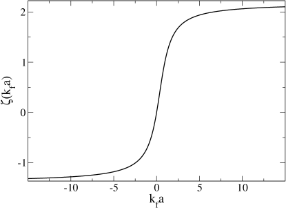
Figure 1: The density-dependent interaction strength function $\zeta(k_{f}a)$ is shown plotted versus $k_{f}a$.

Fig. 1 shows the behavior of this interaction as a function of $k_{f}a$.

Eq. 23 implies that

$$\left\langle\Phi_{\lambda}\left|V_{int}\left(R^{\prime},\Omega\right)\right|\Phi_{\lambda}\right\rangle=\left\langle D_{l_{efff}}\left(\vec{r}_{1},\vec{r}_{2},...,\vec{r}_{N}\right)\left|\sum_{i>j}U_{int}\left(\vec{r}_{ij}\right)\right|D_{l_{eff}}\left(\vec{r}_{1},\vec{r}_{2},...,\vec{r}_{N}\right)\right\rangle_{3N}$$

Owing to the exchange anti-symmetry of the determinantal wavefunction and the orthogonality of the single atom wave functions (see Ref. Cowan (1981) for details), this becomes

$$\left\langle\Phi_{\lambda}\left|V_{int}\left(R^{\prime},\Omega\right)\right|\Phi_{\lambda}\right\rangle =\dfrac{1}{2}\sum_{i,j=1}^{N}\left[\int\left|\psi_{i}\left(\vec{r}_{1}\right)\right|^{2}U_{int}\left(\vec{r}_{12}\right)\left|\psi_{j}\left(\vec{r}_{2}\right)\right|^{2}d^{2}r_{1}d^{3}r_{2}\right.$$

$$-\left.\delta_{m_{s_{i}}m_{s_{j}}}\int\psi_{i}^{\ast}\left(\vec{r}_{1}\right)\psi_{j}\left(\vec{r}_{1}\right)U_{int}\left(\vec{r}_{12}\right)\psi_{j}^{\ast}\left(\vec{r}_{2}\right)\psi_{i}\left(\vec{r}_{2}\right)d^{3}r_{1}d^{3}r_{2}\right]$$

Here $\psi_{i}\left(\vec{r}\right)$ is the spatial state of an atom in the $i$th orbital in the spin substate defined by $m_{s_{i}}$ and the sum runs over all the single particle states in the original determinant. Substituting Eq. 24 for the interaction and using the $\delta$-function to simplify one of the integrals gives

$$\left\langle\Phi_{\lambda}\left|V_{int}\left(R^{\prime},\Omega\right)\right|\Phi_{\lambda}\right\rangle=\dfrac{1}{2}\dfrac{4\pi\hbar^{2}}{m}\sum_{i,j=1}^{N}\left(1-\delta_{m_{s_{i}}m_{s_{j}}}\right)\int\left|\psi_{i}\left(\vec{r}_{1}\right)\right|^{2}\left|\psi_{j}\left(\vec{r}_{1}\right)\right|^{2}\dfrac{\zeta\left(k_{f}\left(\vec{r}_{1}\right)a\right)}{k_{f}\left(\vec{r}_{1}\right)}d^{3}r_{1}$$ (27)

If we sum over all possible spin projections $\delta_{m_{s_{i}}m_{s_{j}}}$ and remember that we have assumed an equal distribution of atoms in each spin substate we arrive at

$$\left\langle\Phi_{\lambda}\left|V_{int}\left(R^{\prime},\Omega\right)\right|\Phi_{\lambda}\right\rangle=\dfrac{4\pi\hbar^{2}}{m}\int\dfrac{\zeta\left[k_{f}\left(\vec{r}\right)a\right]}{k_{f}\left(\vec{r}\right)}\left[\rho_{l_{eff}}^{\left(1\right)}\left(\vec{r}\right)\right]^{2}d^{3}r.$$ (28)

Here we have used the definition of the density of a single spin component

$$\rho_{l_{eff}}^{\left(1\right)}\left(\vec{r}\right)=\sum_{i}^{N/2}\left|\psi_{n_{i}\ell_{i}m_{i}}\left(\vec{r}\right)\right|^{2}.$$

In the Thomas-Fermi approximation, which should be exact for non-interacting oscillator states in the large $N$ limit, this density is given in oscillator units ($l_{0}=\hbar\omega=1$) by

$$\rho_{l_{eff}}^{\left(1\right)}\left(\vec{r}\right)=\dfrac{1}{6\pi^{2}l_{eff}^{3}}\left(2\mu\right)^{3/2}\left(1-\dfrac{r^{2}}{2l_{eff}^{2}\mu}\right)^{3/2}$$ (29)

where $\mu=\left(3N\right)^{1/3}$ is the chemical potential at zero temperature of $N$ non-interacting fermions divided equally between two different spin substates. We may also note from Eq. 22 that in oscillator units, $l_{eff}=R^{\prime}.$ Inserting Eq. 25 and $k_{f}\left(\vec{r}\right)=\left[6\pi^{2}\rho_{leff}^{\left(1\right)}\left(\vec{r}\right)\right]^{1/3}$ and making a change of variables in the integral, Eq. 28 becomes

$$\left\langle\Phi_{\lambda}\left|V_{int}\left(R_{0}^{\prime},\Omega\right)\right|\Phi_{\lambda}\right\rangle =\dfrac{64N^{4/3}}{3^{2/3}\pi^{2}R^{\prime 2}}f\left(\dfrac{k_{f}^{0}a}{R^{\prime}}\right),$$ (30)

$$\text{where }f\left(\dfrac{k_{f}^{0}a}{R^{\prime}}\right) \equiv\int_{0}^{1}y^{6}\sqrt{1-y^{2}}\zeta\left(\dfrac{k_{f}^{0}a}{R^{\prime}}y\right)dy.$$

Here $k_{f}^{0}$ is the peak Fermi wave number for $N$ non-interacting atoms, i.e. $k_{f}^{0}=\left[6\pi^{2}\rho_{l_{0}}^{\left(1\right)}\left(0\right)\right]^{1/3}=\sqrt{2\left(3N\right)^{1/3}}$. Observe that the only parameter in this expression is $k_{f}^{0}a$ which is dimensionless. Inserting Eq. 30 into Eq. 17 now gives the final effective hyperradial potential in the $N\gg 1$ limit.

$$\dfrac{V_{eff}\left(R^{\prime}\right)}{E_{NI}}\rightarrow\dfrac{1}{2R^{\prime 2}}+\dfrac{1}{2}R^{\prime 2}+\dfrac{256}{9\pi^{2}R^{\prime 2}}f\left(\dfrac{k_{f}^{0}a}{R^{\prime}}\right).$$ (31)

For $\left|k_{f}^{0}a\right|\ll R^{\prime}$ the integral may be evaluated exactly using Eq. 26 giving

$$\dfrac{V_{eff}\left(R^{\prime}\right)}{E_{NI}}\rightarrow\dfrac{1}{2R^{\prime 2}}+\dfrac{1}{2}R^{\prime 2}+\dfrac{4096k_{f}^{0}a}{2835\pi^{2}R^{\prime 3}}$$ (32)

which is exactly the behavior predicted in Ref. Rittenhouse et al. (2006) using non-renormalized zero-range interactions.

IV.1 Repulsive effective interactions, $a>0$

Here we explore the behavior of the DFG under a repulsive effective potential where the two-body scattering length, $a$, is positive. The renormalized description of the interactions used here and in Ref. von Stecher and Greene (2006) is only accurate if the real two-body interactions are purely repulsive or if the gas is somehow prevented from forming into molecular dimer states. In other words we can only look at a gas of atoms not of molecules. Fig. 2, which shows $V_{eff}$ for several positive two-body scattering lengths, also shows an example of the bare non-renormalized effective potential. As one would expect, the repulsive interactions cause the gas to push out against itself and against the trap walls, which increases the overall energy and size of the gas.

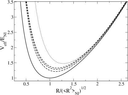
Figure 2: The dimensionless ratio of the effective hyperradial potential to the non-interacting total energy is plotted as a function of the dimensionless rescaled hyperradius, for several different repulsive interaction strengths. The non-interacting limit $k_{f}^{0}a=0$ is shown as the sold curve; the dashed curves show the renormalized effective potential for (bottom to top) $k_{f}^{0}a=2$, $k_{f}^{0}a=5$ and $k_{f}^{0}a=50$. Also shown is the non-renormalized effective potential with $k_{f}^{0}a=5$ (dotted curve).

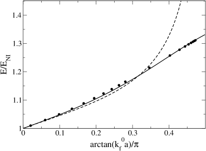
Figure 3: The ground state energy of the DFG in units of the non-interacting energy predicted by the K harmonic method (solid line) is plotted versus $\arctan\left(k_{f}^{0}a\right)/\pi$ and compared with that predicted by the Hartree-Fock method with 2280 atoms (circles). The dashed line is the ground state energy predicted by the K harmonic method using the bare Fermi pseudo-potential.

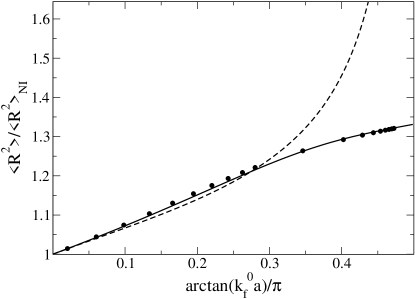
Figure 4: The ground state average squared hyperradius of the two-component DFG in the large-N limit, divided by the non-interacting value for this quantity, is plotted versus $\arctan\left(k_{f}^{0}a\right)/\pi$. Also shown are the values predicted by the Hartree-Fock method with 2280 atoms (circles). The dashed line is the ground state energy predicted by the K harmonic method using the bare Fermi pseudo-potential.

The true ground state energy would be found by solving Eq. 16 for the lowest eigenvalue, but if we examine $m^{\ast}$ in the large $N$ limit one can see that the second derivative term becomes negligible. The ground state energy and hyperradius can thus be found by minimizing the effective potential $V_{eff}\left(R^{\prime}\right).$ Figs. 3 and 4 show the energy and average squared hyperradius of the minimum of $V_{eff}$ as functions of $k_{f}^{0}a$, compared to those same values calculated using the bare non-renormalized effective potential given by Eq. 32. Also shown are the ground state energy and average hyperradius squared predictions from the Hartree-Fock method using the renormalized interaction. As the interaction gets stronger the renormalized energies and hyperradii flatten out and approach a constant in the unitarity limit. This behavior will be examined more carefully in a Section IV(C). For $k_{f}^{0}a\ll 1$ the Fermi pseudo-potential approximation is in good quantitative agreement with the renormalized interactions, but diverges dramatically as $k_{f}^{0}a\rightarrow\infty$. This dramatizes the breakdown of the non-renormalized zero-range approximation, which overestimates the interaction strength as the unitarity regime is approached.

IV.2 Attractive effective interactions, $a<0$

Fig. 5 shows the behavior of the effective potential for some attractive values of the two-body scattering length, along with an example of the non-renormalized effective potential. The decisive qualitative importance of the renormalization is now apparent; for attractive non-renormalized interactions the interaction term in the effective potential will always take over as $R^{\prime}\rightarrow 0$ which creates an inner collapse region where the ground state energy of the gas diverges toward $-\infty$ and the gas lives in a metastable outer potential well. In contrast, the renormalized effective potential has no such collapse phenomenon, and the ground state of the gas is in a global minimum. This behavior will be discussed further in Section IV(C).

Figs. 6 and 7 show the ground state energy and average hyperradius squared of the system compared to the non-renormalized values.

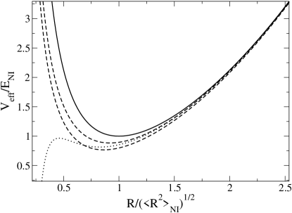
Figure 5: The effective potential in units of the non-interacting energy is plotted versus the hyperradius in units of $\sqrt{\left\langle R^{2}\right\rangle_{NI}}$, for several interaction strengths. The non-interacting limit $k_{f}^{0}a=0$ is shown as the sold curve and the dashed curves show the renormalized effective potential for (top to bottom) $k_{f}^{0}a=-1$ and $k_{f}^{0}a=-5$. Also shown is the non-renormalized effective potential with $k_{f}^{0}a=-1$ (dotted curve).

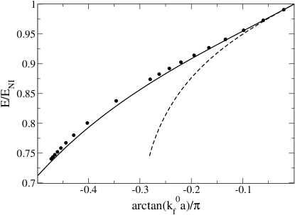
Figure 6: The ground state energy of the DFG, predicted by the K harmonic method in units of the non-interacting energy (solid line) is shown as a function of $\arctan\left(k_{f}^{0}a\right)$/$\pi$ as a solid line. Also shown is that predicted by the Hartree-Fock method for 2280 atoms (circles). The dashed line is the ground state energy predicted by the K harmonic method using the bare Fermi pseudopotential.

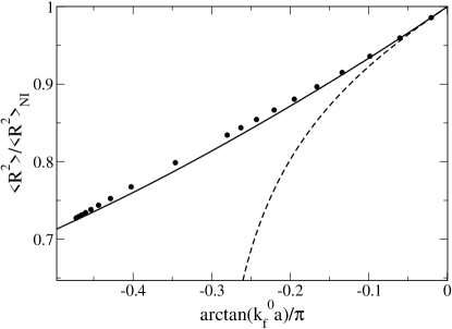
Figure 7: The ground state average hyperradius squared of the DFG in units of the non-interacting average hyperradius squared predicted by the K harmonic method (solid line) is shown plotted against $\arctan\left(k_{f}^{0}a\right)/\pi$ compared with that predicted by the Hartree-Fock method with 2280 atoms (circles). The dashed line is the ground state energy predicted by the K harmonic method using the bare Fermi pseudopotential.

The effects of renormalization for attractive interaction are even more striking than in the repulsive interaction case. Without renormalization the metastable region of the effective potential disappears for $k_{f}^{0}a<-1.21$ Rittenhouse et al. (2006) and the gas has no barrier to prevent it from falling into the central collapse region. With renormalization, as $k_{f}^{0}a\rightarrow-\infty$ the energy and average hyperradius squared go towards a fixed value. Figs. 6 and 7 also show the ground state energy and average squared hyperradius predictions from the Hartree-Fock method. For $\left|k_{f}^{0}a\right|\ll 1$ the non-renormalized and renormalized values are in good agreement, but as $k_{f}^{0}a\rightarrow-1.21$ the Fermi-pseudopotential diverges away from the renormalized interaction results. In fact, Ref. Rittenhouse et al. (2006) predicts a collapse of the gas for non-renormalized interactions at $k_{f}^{0}a=-1.21$. Just before the point of collapse the ground state energy is predicted to be $E=\sqrt{5}E_{NI}/3=0.745E_{NI}$. Not only does the renormalized effective potential cut off the collapse behavior, it also allows the gas to reach a lower energy than it would be able to without the density dependence. In other words, if the interaction coefficient in $U_{int}\left(\vec{r}_{ij}\right)$ were not density-dependent, but merely involved a cut off as $k_{f}^{0}a\rightarrow-\infty,$ the gas would not be able to reach the unitarity energy before collapsing.

IV.3 Unitarity regime

In this section we explore the behavior of $V_{eff}$ in the strong interaction regime, i.e. $a\rightarrow\pm\infty$. Examining Eq. 30 shows that the unitarity limit is when $\left|k_{f}^{0}a\right|\gg R^{\prime}$.

$$\dfrac{\left\langle\Phi_{\lambda}\left|V_{int}\left(R_{0}^{\prime},\Omega\right)\right|\Phi_{\lambda}\right\rangle}{E_{NI}} \rightarrow\dfrac{256\zeta_{\pm}}{9\pi^{2}R^{\prime 2}}\int_{0}^{1}y^{6}\sqrt{1-y^{2}}dy$$

$$=\dfrac{5\zeta_{\pm}}{9\pi R^{\prime 2}}$$

where $\zeta_{\pm}$ is the maximum ($+$) or minimum ($-$) value acquired by the interaction function $\zeta\left(k_{f}a\right)$. This gives a total effective potential of

$$\dfrac{V_{eff}\left(R^{\prime}\right)}{E_{NI}} \rightarrow\dfrac{1}{2}R^{\prime 2}+\dfrac{1/2+5\zeta_{\pm}/9\pi}{R^{\prime 2}}$$ (33)

$$=\left\{\begin{array}[c]{ccc}\dfrac{1}{2}R^{\prime 2}+\dfrac{0.886}{R^{\prime 2}}&\text{for}&k_{f}^{0}a\gg R^{\prime}\\ &&\\ \dfrac{1}{2}R^{\prime 2}+\dfrac{0.254}{R^{\prime 2}}&\text{for}&-k_{f}^{0}a\gg R^{\prime}\end{array}\right..$$ (37)

The hyperradius is a collective coordinate so that, as $R\rightarrow 0$, all of the atoms in the system are forced to the center of the trap, which increases the density of the system. Thus, for small hyperradii, we expect $V_{eff}$ to act like Eq. 33. In fact, the dashed curves in Figs. 2 and 5 show that as $R^{\prime}\rightarrow 0$ the renormalized effective potential curves start to behave the same, independently of $a$. Alternatively if the two-body scattering length approaches $-\infty$, e.g. near a resonance, then we can expect the interaction to approach Eq. 33 for all hyperradii.

In the case where $k_{f}^{0}a\rightarrow\pm\infty$ the effective potential takes on the form of Eq. 33. Minimization of $V_{eff}$ as a function of $R^{\prime}$ gives a ground state energy:

$$\dfrac{E}{E_{NI}} =\sqrt{1+10\zeta_{\pm}/9\pi}$$ (38)

$$=\left\{\begin{array}[c]{ccc}1.331&for&a\rightarrow\infty\\ 0.712&for&a\rightarrow-\infty\end{array}\right..$$ (41)

The average hyperradius of the gas is described by the value of the hyperradius at this minimum which is given by

$$R_{\min}^{\prime} =\left(1+10\zeta_{\pm}/9\pi\right)^{1/4}$$ (42)

$$=\left\{\begin{array}[c]{ccc}1.154&for&a\rightarrow\infty\\ 0.844&for&a\rightarrow-\infty\end{array}\right.$$ (45)

At first glance this may seem strange, one might expect the behavior to be smooth across a resonance, and the energy to connect smoothly from the $a\rightarrow-\infty$ limit to the $a\rightarrow\infty$ limit Astrakharchik et al. (2004). But the density-dependent renormalization used here only applies to a degenerate Fermi gas of atoms and does not allow for the incorporation of higher order correlations, i.e. the formation of diatomic molecules. Presumably there is another branch in the renormalization that will match continuously with the $a\rightarrow-\infty$ limit (for a more complete discussion see section II of Ref. von Stecher and Greene (2006)).

Another quantity of interest is the chemical potential of the interacting gas at unitarity, given by

$$\mu_{u}=\dfrac{\hbar^{2}k_{f}^{2}\left(0\right)}{2m}\left(1+\beta\right),$$

where $\beta$ is a universal parameter. From the single spin component density given in Eq. 29 we find that the interacting peak Fermi wavenumber is

$$k_{f}\left(0\right)=\dfrac{k_{f}^{0}}{R_{\min}^{\prime 2}}.$$ (46)

Further, from Eqs. 38 and 42, the ratio of the chemical potential of the interacting unitarity-limit gas to that of the non-interacting gas can be written in terms of the rescaled hyperradius as:

$$\dfrac{\mu_{u}}{\mu}=\dfrac{E}{E_{NI}}=R_{\min}^{\prime 2}.$$ (47)

Solution of Eqs. 46 and 47 in the $a\rightarrow-\infty$ limit yields

$$\beta=10\zeta_{-}/9\pi=-0.49.$$

This value of $\beta$ coincides, not surprisingly, with the value predicted by the renormalized Hartree-Fock calculation of Ref. von Stecher and Greene (2006). Even though neither Ref. von Stecher and Greene (2006) nor our present treatment explicitly incorporates Cooper-type fermion pairing, this unitarity limit $\beta$ is in fair agreement with quantum Monte Carlo estimates that have obtained $\beta=-0.58$ (Ref. Astrakharchik et al. (2004).) and $-0.56$ (Ref.Chang et al. (2004) ).

IV.4 Breathing mode excitations

Refs. Bohn et al. (1998); Rittenhouse et al. (2006) showed that one of the strengths of the K harmonic method is its ability to predict the lowest radial excitation, the breathing mode. With the effective potential derived here, this frequency is found by simply examining the second order Taylor series about the minimum in $V_{eff}\left(R^{\prime}\right)$ and comparing the resulting Hamiltonian to that of an oscillator. The approximate Hamiltonian is given by

$$H=\dfrac{-1}{2m^{\ast}}\dfrac{d^{2}}{dR^{\prime 2}}+\dfrac{E_{GS}}{E_{NI}}+\dfrac{1}{2E_{NI}}\left.\dfrac{\partial^{2}V_{eff}}{\partial R^{\prime 2}}\right|_{R^{\prime}=R_{\min}^{\prime}}\left(R^{\prime}-R_{\min}^{\prime}\right)^{2}$$ (48)

where $E_{GS}$ is the ground state energy of the system and $R_{\min}^{\prime}$ is the hyperradius that minimizes $V_{eff}$ scaled by $\sqrt{\left\langle R^{2}\right\rangle_{NI}}$. this can be recast as the oscillator Hamiltonian

$$H_{ho}=\dfrac{-1}{2m^{\ast}}\dfrac{d^{2}}{dR^{\prime 2}}+\dfrac{E_{GS}}{E_{NI}}+\dfrac{1}{2}m^{\ast}\omega_{0}^{\prime 2}\left(R^{\prime}-R_{\min}^{\prime}\right)^{2}.$$ (49)

Here $\omega_{0}^{\prime}$ is given by the second derivative of the $V_{eff}$ at the minimum:

$$\omega_{0}^{\prime}=\sqrt{\dfrac{1}{m^{\ast}E_{NI}}\left.\dfrac{\partial^{2}V_{eff}}{\partial R^{\prime 2}}\right|_{R^{\prime}=R_{\min}^{\prime}}}.$$ (50a)

This parameter is the breathing mode frequency in units of $$E_{NI}/\hbar m^{\ast}\rightarrow E_{NI}^{2}/\hbar^{2}\omega^{2} N \omega_{0}$$. Taking in the large limit gives the breathing mode frequency, :

$$\omega_{0}=\omega\sqrt{\dfrac{1}{E_{NI}}\left.\dfrac{\partial^{2}V_{eff}}{\partial R^{\prime 2}}\right|_{R^{\prime}=R_{\min}^{\prime}}}$$ (51)

where $\omega$ is the oscillator frequency of the trap. Fig. 8 shows the breathing mode frequency in units of the oscillator frequency compared to that calculated using non-renormalized interactions. Of course the breathing mode frequency in the non-interacting limit is $\omega_{0}=2\omega$, but surprisingly, the frequency turns over and returns to the non-interacting value as $k_{f}^{0}a\rightarrow\pm\infty$. Upon inserting the second derivative of Eq. 33, the effective potential as $k_{f}^{0}a\rightarrow\pm\infty$ we obtain

$$\omega_{0}=\omega\sqrt{\dfrac{1}{E_{NI}}\left(1+\left.3\dfrac{1+10\zeta_{\pm}/9\pi}{R^{\prime 4}}\right|_{R^{\prime}=R_{\min}^{\prime}}\right)}.$$ (52)

When the minimum hyperradius from Eq. 42 is plugged in, this implies that the unitarity limits for the breathing mode frequency are both $\omega_{0}=2\omega$. This unitarity behavior has also been predicted in Ref. Werner and Castin (2006).

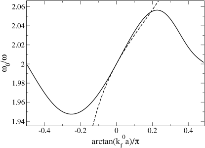
Figure 8: The breathing mode frequency $\omega_{0}$ is shown in units of the trap frequency $\omega$ versus $\arctan\left(k_{f}^{0}a\right)/\pi$ . The solid curve shows the breathing mode predicted using the renormalized interaction while the dashed curve shows the prediction based on the bare Fermi pseudo-potential.

V Multiple spin components

Next consider what happens when the atoms in the gas are equally distributed among an arbitrary number $\chi$ of spin substates. First, we assume, in order to limit parameter space, that the s-wave scattering length between two atoms in any two different spin states has the same value, $a$. Also we neglect the possibility of inelastic collisions, e.g. of the type:

$$\left|m_{1}=\dfrac{3}{2}\right\rangle+\left|m_{2}=-\dfrac{3}{2}\right\rangle\rightarrow\left|m_{1}^{\prime}=\dfrac{1}{2}\right\rangle+\left|m_{2}^{\prime}=-\dfrac{1}{2}\right\rangle.$$

To proceed, we must also address the question of what density should go into the renormalized interactions. A particle in spin state $i$ cannot interact with any other particle in the same spin state by the zero range approximation, but the density that determines $k_{f}\left(r\right)$ in the renormalization function $\zeta$ might be chosen in various alternative ways, and we have not yet developed a unique criterion to specify the appropriate renormalization in this context. As an initial exploration, we make the assumption that the density of the component that particle $i$ is interacting with is the density that modifies the interaction, i.e.

$$V\left(r_{ij}\right)=\dfrac{4\pi\hbar^{2}\zeta\left[k_{f}^{\left(j\right)}\left(\vec{r}_{i}\right)a\right]}{k_{f}^{\left(j\right)}\left(\vec{r}_{i}\right)}\delta\left(\vec{r}_{i}-\vec{r}_{j}\right)$$

where $k_{f}^{\left(j\right)}\left(\vec{r}\right)=\left[6\pi^{2}\rho^{\left(j\right)}\left(\vec{r}\right)\right]^{1/3}$ is the Fermi wave number of the spin component that particle $j$ belongs to.

The derivation following this assumptions the same as that for the two-component gas, up to Eq. 27. The only added pieces of information needed are the common density of each component in the effective trap with oscillator length $l_{eff}$, the chemical potential, the non-interacting ground state energy and the average hyperradius squared for the system with $\chi$ spin substates in the large $N$ limit:

$$\rho_{l_{eff}}^{\left(1\right)}\left(\vec{r}\right) =\dfrac{1}{6\pi^{2}l_{eff}^{3}}\left(2\mu\right)^{3/2}\left(1-\dfrac{r^{2}}{2l_{eff}^{2}\mu}\right)^{3/2}$$ (53)

$$\mu =\left(\dfrac{6N}{\chi}\right)^{1/3}$$ (54)

$$E_{NI} =\hbar\omega\dfrac{\left(6N\right)^{4/3}}{\chi^{1/3}8}$$ (55)

$$\left\langle R^{2}\right\rangle_{NI} =\dfrac{\hbar}{m\omega}\dfrac{\left(6N\right)^{4/3}}{\chi^{1/3}8N}.$$ (56)

The sum over spin substates in Eq. 27 results in a factor of $\chi\left(\chi-1\right)$, leaving

$$\left\langle\Phi_{\lambda}\left|V_{int}\left(R^{\prime},\Omega\right)\right|\Phi_{\lambda}\right\rangle=\dfrac{4\pi\hbar^{2}}{m}\dfrac{\chi\left(\chi-1\right)}{2}\int\dfrac{\zeta\left[k_{f}\left(\vec{r}\right)a\right]}{k_{f}\left(\vec{r}\right)}\left[\rho_{l_{eff}}^{\left(1\right)}\left(\vec{r}\right)\right]^{2}d^{3}r.$$ (57)

Another change of integration variables which gives the effective hyperradial potential as

$$\dfrac{V_{eff}\left(R^{\prime}\right)}{E_{NI}} =\dfrac{1}{2R^{\prime 2}}+\dfrac{1}{2}R^{\prime 2}+\left(\chi-1\right)\dfrac{64N^{4/3}}{3^{2/3}\pi^{2}R^{\prime 2}}f\left(\dfrac{k_{f}^{0}a}{R^{\prime}}\right).$$ (58)

$$f\left(\dfrac{k_{f}^{0}a}{R^{\prime}}\right) \equiv\int_{0}^{1}y^{6}\sqrt{1-y^{2}}\zeta\left(\dfrac{k_{f}^{0}a}{R^{\prime}}y\right)dy.$$

Comparison with Eq. 31, the effective potential for the two component gas, demonstrates that the extra spin components increase the strength of the interaction by a factor of $\chi-1$.

In the limit where $k_{f}^{0}a\rightarrow-\infty$ the effective potential limits to

$$\dfrac{V_{eff}\left(R^{\prime}\right)}{E_{NI}}\rightarrow\dfrac{1}{2}R^{\prime 2}+\dfrac{1+10\left(\chi-1\right)\zeta_{-}/9\pi}{2R^{\prime 2}}$$ (59)

Taking $\chi=3$ yields

$$\dfrac{V_{eff}\left(R^{\prime}\right)}{E_{NI}} \rightarrow\dfrac{1}{2}R^{\prime 2}+\dfrac{1-20\zeta_{-}/9\pi}{2R^{\prime 2}}$$ (60)

$$=\dfrac{1}{2}R^{\prime 2}+\dfrac{0.00772}{R^{\prime 2}}.$$

In this limit the barrier preventing the gas from falling in to the center of the trap, i.e. $R^{\prime}\rightarrow 0$, is very weak. The unitarity energy and average hyperradius are given by

$$\allowbreak\dfrac{E}{E_{NI}} =\sqrt{1+20\zeta_{-}/9\pi}=0.124$$

$$\dfrac{R_{\min}}{\sqrt{\left\langle R^{2}\right\rangle_{NI}}} =\left(1+20\zeta_{-}/9\pi\right)^{1/4}=0.352.$$

Since the K harmonic method is intrinsically a variational calculation, it is very possible that a better calculation, for example using the Hartree-Fock method, might show that the 3 component gas becomes mechanically unstable in the unitarity limit Heiselberg (2001). In other words the three component gas might collapse in a manner similar to that of the Bosenova Bohn et al. (1998); Shuryak (1996); Stoof (1997); Bradley et al. (1995); Donley et al. (2001).

With $\chi=4$ the effective potential at $k_{f}^{0}a\rightarrow-\infty$ becomes entirely attractive

$$\dfrac{V_{eff}\left(R^{\prime}\right)}{E_{NI}} \rightarrow\dfrac{1}{2}R^{\prime 2}+\dfrac{1-30\zeta_{-}/9\pi}{2R^{\prime 2}}$$ (61)

$$=\dfrac{1}{2}R^{\prime 2}-\dfrac{\allowbreak 0.238}{R^{\prime 2}}$$

meaning that the gas is predicted to collapse down toward $R^{\prime}\rightarrow 0$. Presumably some very rich and complex dynamics (cluster formation, inelastic collisions, etc.) occur during this process, but our K harmonic trial wave function is too simple to describe these phenomena. When the local minimum in $V_{eff}\left(R^{\prime}\right)$ becomes a saddle point the gas is no longer mechanically stable and is free to collapse. This occurs at a critical interaction strength of $k_{f}a_{c}=-0.657$.

VI Summary and prospects

We have shown that applying the variational hyperspherical treatment of Ref. Rittenhouse et al. (2006) to a density-dependent, zero-range, s-wave interaction produces a unique, physically intuitive picture of the behavior of gas. By fixing the hyperangular behavior of the gas, in the large atom number limit, a simple 1D effective potential in a collective coordinate, the hyperradius $R$ was produced. The ground state energy and rms radius of the two component gas predicted by this method are in excellent agreement with those predicted using the Hartree-Fock method. The ground state energy of the two component gas goes to a finite, unitarity limit as the two-body scattering length $a$ diverges to $+\infty$. Due to the inability of our hyperspherical trial function and the renormalized, density-dependent interaction to describe two-body bound states, the method only applies (at this level of our development) to a degenerate Fermi gas of atoms. In the $a\rightarrow-\infty$ the two component gas has a stable ground state and avoids the collapsing behavior predicted for the bare Fermi pseudo-potential, and has a ground state energy of $0.73$ times the ground state energy of $N$ non-interacting fermions in an isotropic oscillator trap. This energy is lower than the minimum energy that could be reached before collapse, which would be predicted without density-dependent interactions. In the unitarity limit, the lowest radial excitation frequency, the breathing mode frequency, for the two component gas is the same as the non-interacting value in both the positive and negative asymptotic scattering length limits.

The effective potential for a three component gas has a weak hyperradial barrier in the $a\rightarrow-\infty$ limit, which just barely prevents collapse of the gas. Because of the variational nature of the K-harmonic method, a better approximation of the wavefunction, as in the Hartree-Fock method, might conceivably allow the three component system to collapse. For four or more spin components the repulsive barrier becomes attractive in the $a\rightarrow-\infty$ and the gas is predicted to collapse in a manner similar to the Bosenova Bohn et al. (1998); Shuryak (1996); Stoof (1997); Bradley et al. (1995); Donley et al. (2001). Some uncertainty about this prediction still exists, however, because we have not yet validated our renormalization procedure for DFGs containing more than two spin components. Here, the interactions between different spin components was assumed to be the same for all possible combinations. A more accurate treatment would include different two-body scattering lengths for different combinations of spin components, though if all scattering lengths are large and negative, the prediction of instability would still apply. Higher-order correlations, such as BEC or BCS pairing are beyond the scope of this work, and relegated to future publication.

References

- Fermi (1936) E. Fermi, Ric. Sci. 7, 13 (1936).
- Bruun and Burnett (1998) G.M. Bruun and K. Burnett, Phys. Rev. A 58, 2427 (1998).
- Houbiers et al. (1997) M. Houbiers, R. Ferwerda, H.T.C. Stoof, W.I. McAlexander, C.A. Sackett, and R.G. Hulet, Phys. Rev. A 56, 4864 (1997).
- Roth and Feldmeier (2001) R. Roth and H. Feldmeier, Phys. Rev. A 64, 43603 (2001).
- Bartenstein et al. (2004) M. Bartenstein, A. Altmeyer, S. Riedl, S. Jochim, C. Chin, J.H. Denschlag, and R. Grimm, Phys. Rev. Lett. 92, 120401 (2004).
- Bourdel et al. (2004) T. Bourdel, L. Khaykovich, J. Cubizolles, J. Zhang, F. Chevy, M. Teichmann, L. Tarruell, S.J.J.M.F. Kokkelmans, and C. Salomon, Phys. Rev. Lett. 93, 50401 (2004).
- Kinast et al. (2004) J. Kinast, S.L. Hemmer, M.E. Gehm, A. Turlapov, and J.E. Thomas, Phys. Rev. Lett. 92, 150402 (2004).
- Regal et al. (2004) C.A. Regal, M. Greiner, and D.S. Jin, Phys. Rev. Lett. 92, 40403 (2004).
- Zwierlein et al. (2004) M.W. Zwierlein, C.A. Stan, C.H. Schunck, S.M.F. Raupach, A.J. Kerman, and W. Ketterle, Phys. Rev. Lett. 92, 120403 (2004).
- von Stecher and Greene (2006) J. von Stecher and C. H. Greene, eprint cond-mat/0610848 (2006).
- Rittenhouse et al. (2006) S.T. Rittenhouse, M.J. Cavagnero, J. von Stecher, and C.H. Greene, Phys. Rev. A 74, 053624 (2006).
- Avery (1989) J. Avery, Hyperspherical Harmonics: Applications in Quantum Theory (Kluwer Academic Publishers, Norwell, MA, 1989).
- Fano and Rau (1986) U. Fano and A. Rau, Atomic Collisions and Spectra (Academic Press, Orlando, FL, 1986).
- Smirnov and Shitikova (1977) Y. F. Smirnov and K. V. Shitikova, Sov. J. Part. Nucl. 8, 44 (1977).
- Bohn et al. (1998) J. L. Bohn, B. D. Esry, and C. H. Greene, Phys. Rev. A 58, 584 (1998).
- Timofeyuk (2004) N. K. Timofeyuk, Phys. Rev. C 69, 034336 (2004).
- (17) See, for instance D. Z. Goodson, M. Lopez-Cabrera, D. R. Herschbach, J. D. Morgan III, J. Chem. Phys. 97, 8481 (1992); J. G. Loeser, J. H. Summerfield, A. L. Tan, Z. Zheng, J. Chem. Phys. 100, 5036 (1994); M. Dunn and D. K. Watson, Annals of Physics 251, 266-318 and 319-336 (1996).
- Cowan (1981) R. D. Cowan, The Theory of Atomic Structure and Spectra (University of California Press, Los Angeles, CA, 1981).
- Astrakharchik et al. (2004) G.E. Astrakharchik, J. Boronat, J. Casulleras, and S. Giorgini, Phys. Rev. Lett. 93, 200404 (2004).
- Chang et al. (2004) S.Y Chang, V.R. Pandharipande, J. Carlson, and K.E. Schmidt, Phys. Rev. A 70, 43602 (2004).
- Werner and Castin (2006) F. Werner and Y. Castin, Phys. Rev. A 74, 53604 (2006).
- Heiselberg (2001) H. Heiselberg, Phys. Rev. A 63, 43606 (2001).
- Bradley et al. (1995) C.C. Bradley, C.A. Sackett, J.J. Tollett, and R.G. Hulet, Phys. Rev. Lett. 75, 1687 (1995).
- Donley et al. (2001) E. Donley, N. Claussen, S. Cornish, J. Roberts, E. Cornell, and C. Wieman, Nature 412, 295 (2001).
- Shuryak (1996) E.V. Shuryak, Phys. Rev. A 54, 3151 (1996).
- Stoof (1997) H. Stoof, J. Stat. Phys. 87, 1353 (1997).