Evaluation of three methods for calculating statistical significance when incorporating a systematic uncertainty into a test of the background-only hypothesis for a Poisson process

Abstract

Hypothesis tests for the presence of new sources of Poisson counts amidst background processes are frequently performed in high energy physics (HEP), gamma ray astronomy (GRA), and other branches of science. While there are conceptual issues already when the mean rate of background is precisely known, the issues are even more difficult when the mean background rate has non-negligible uncertainty. After describing a variety of methods to be found in the HEP and GRA literature, we consider in detail three classes of algorithms and evaluate them over a wide range of parameter space, by the criterion of how close the ensemble-average Type I error rate (rejection of the background-only hypothesis when it is true) compares with the nominal significance level given by the algorithm. We recommend wider use of an algorithm firmly grounded in frequentist tests of the ratio of Poisson means, although for very low counts the over-coverage can be severe due to the effect of discreteness. We extend the studies of Cranmer, who found that a popular Bayesian-frequentist hybrid can undercover severely when taken to high $Z$ values. We also examine the profile likelihood method, which has long been used in GRA and HEP; it provides an excellent approximation in much of the parameter space, as previously studied by Rolke and collaborators.

, ,

1 Introduction

The incorporation of systematic uncertainties into hypothesis tests (and by implication into confidence intervals and limits) remains a murky area of data analysis in spite of much study in the professional statistics community and in high energy physics, in gamma ray astronomy, and in other branches of science [1]. Exact methods using the frequentist definition of probability typically do not exist, while purely Bayesian methods, as commonly used in high energy physics, invoke uniform priors which make the resulting probability statements hard to interpret if not completely arbitrary.

The foundational issues already arise in startlingly simple prototype problems such as the one that we examine in this paper: $n_{\rm on}$ events are observed from the Poisson process with mean $\mu_{\rm s}+\mu_{\rm b}$, where $\mu_{\rm s}$ is the unknown parameter of interest (the mean number of signal events), while $\mu_{\rm b}$ is the mean number of background events (mimicking signal events), measured to have a value $\hat{\mu}_{\rm b}$ with some uncertainty from subsidiary observations. One wishes to test the hypothesis $H_{0}$ that $\mu_{\rm s}=0$, i.e., that the observed number of events is statistically consistent with being all background. In this paper, we focus on the significance level $\alpha$ of the hypothesis test, also known as the size of the test, and in particular consider the very small values of $\alpha$ corresponding to a statistical significance of up to five standard deviations. In the formal theory of Neyman-Pearson hypothesis testing, $\alpha$ is specified in advance; once data are obtained, the $p$-value is the smallest value of $\alpha$ for which $H_{0}$ would be rejected. In a real application, the power of the test, which depends on the alternative hypothesis, should be considered as well, but we do not explore that complementary aspect of the test here [2]. Also, we do not address the complex issue of the utility of $p$-values, which is discussed by Berger and others (e.g., Refs. [3, 4]); we merely remind the reader that at best, a $p$-value conveys the probability under $H_{0}$ of obtaining a value of the test statistic at least as extreme as that observed, and that it should not be interpreted as the probability that $H_{0}$ is true. Having said that, given the ubiquity of $p$-values in the literature, we study in detail the efficacy of three methods for calculating $p$-values in the presence of systematic uncertainties.

Frequently the $p$-value is communicated by specifying the corresponding number of standard deviations in a one-tailed test of a Gaussian (normal) variate; i.e., one communicates a $Z$-value (often called $S$ in HEP) given by

$$Z=\Phi^{-1}(1-p)=-\Phi^{-1}(p)$$ (1)

where

$$\Phi(Z)=\frac{1}{\sqrt{2\pi}}\int_{-\infty}^{Z}\,\exp(-t^{2}/2)\,dt\ =\ \frac{1+{\rm erf}(Z/\sqrt{2})}{2},$$ (2)

so that

$$Z=\sqrt{2}\,{\rm erf}^{-1}(1-2p).$$ (3)

Thus, for example, $Z=3$ corresponds to a $p$-value of $1.35\times 10^{-3}$. This relation can be approximated to better than 1% for $Z>1.6$ as

$$Z\approx\sqrt{u-\ln\ u},$$ (4)

where $u=-2\ln(p\sqrt{2\pi})$. (See Appendix B.) This form fortuitously is much more accurate than directly inverting the full asymptotic expansion to second or third order. Asymptotically, $Z$ goes as $\sqrt{-\ln\ p}$ at large $Z$.

If the uncertainty on $\hat{\mu}_{\rm b}$ vanishes (so that $\hat{\mu}_{\rm b}=\mu_{\rm b}$), some controversy exists as to the best way to proceed, but at least in that case there seems to be some clarity about the different methods, their performance, and their merits and demerits. In contrast, if the uncertainty on $\hat{\mu}_{\rm b}$ is non-negligible, then the nature of the subsidiary measurement of $\mu_{\rm b}$ becomes crucial, and the interpretation of results of various recipes (algorithms for computing the $p$-value) becomes much more difficult. We take a pragmatic point of view that the performance of a recipe is of more interest than the foundational solidity of the recipe, and evaluate this performance by the frequentist criterion of how well the nominal significance level of a test corresponds to the true frequency of Type I errors (rejecting $H_{0}$ when it is true).

As in Ref. [5], we consider two variations of this prototype problem (described in Sec. 2), which differ in the specification of the subsidiary measurement of $\mu_{\rm b}$. In the first case, it is a (typically small-integer) Poisson measurement in a signal-free control region, and in the second case it is a Gaussian (normal) measurement with known rms deviation. Section 3 describes the little-used fact [5, 6] that the standard frequentist solution to the ratio-of-Poisson-means problem can be directly applied to the first prototype problem at hand, which makes evaluation of $Z$ easy with modern software tools. In Sec. 4, we outline the frequentist-Bayesian hybrid which is commonly used in HEP, noting its lack of foundational solidity and ambiguity due to choice of the Bayesian prior. We note the remarkable mathematical connection between one choice of prior and the frequentist solution of Sec. 3. In Sec. 5, we explore the profile likelihood method (well-known in HEP as the MINUIT MINOS method [7] and in gamma ray astronomy (GRA) as popularized by Li and Ma [8]), which gives approximate results based on likelihood ratios. In Sec. 6, we briefly describe other methods, and in Sec. 7 we compare some results obtained with all the methods.

In the remaining sections we focus on the three main methods introduced in Secs. 3-5, and study in detail the relations among the computed $Z$ values and the Type I error rates, as one spans the space of true values of the parameters. We conclude in Sec. 10 that the little-used frequentist solution should have much broader use, and we even advocate its prudent use in the second prototype problem, in which it applies only via a rough correspondence. As found in Refs. [9, 10], (which advocate some modifications) the profile likelihood method provides remarkably good results over a wide range of parameters. Given the richness of results even for these simple prototype problems, there remains much work to be done, beyond the scope of this paper, in exploring performance of other recipes and further generalizations to more complicated problems [1, 11, 12, 13].

Appendix A contains a summary of our notation. Appendix B has a derivation of Eqn. 4, followed in Appendix C by a proof of the “remarkable connection” mentioned above. Calculational details of the various $Z$-values are in Appendix D, and some implementation examples are in Appendix E.

2 Two prototype problems differing in the measurement of $\mu_{\rm b}$

2.1 The on/off problem

In the first prototype problem, which we refer to as the “on/off” problem, the subsidiary measurement of $\mu_{\rm b}$ consists of the observation of $n_{\rm off}$ events in a control region where no signal events are expected. In HEP, the control region is commonly referred to as a “sideband” since it is typically a sample of events which is near the signal region in some measured parameter, i.e., in a band of that parameter alongside but disjoint from the parameter values where the signal might exist.

This HEP prototype problem has an exact analog in gamma ray astronomy (GRA), upon which we base our notational subscripts “on” and “off”. The observation of $n_{\rm on}$ photons when a telescope is pointing at a potential source (“on-source”) includes both background and the source, while the observation of $n_{\rm off}$ photons with the telescope pointing at a source-free direction nearby (“off-source”) is the subsidiary measurement. In both the HEP and GRA examples, we let the parameter $\tau$ denote the ratio of the expected means of $n_{\rm off}$ and $n_{\rm on}$ under $H_{0}$, i.e., when $\mu_{\rm on}=\mu_{\rm b}$:

$$\tau\equiv\mu_{\rm off}/\mu_{\rm b}.$$ (5)

In GRA, $\tau$ in the simplest case is the ratio of observing time off/on source (subject to corrections in more complicated cases), while in HEP the calculation of $\tau$ might involve background shapes, efficiencies, etc., determined by Monte Carlo simulation. In the prototype problems studied in detail in this paper we assume that $\tau$ itself is known exactly or with negligible uncertainty. Thus, since the point estimate of $\mu_{\rm off}$ is $n_{\rm off}$, the point estimate of $\mu_{\rm b}$ is

$$\hat{\mu}_{\rm b}=n_{\rm off}/\tau.$$ (6)

2.2 The Gaussian-mean background problem

In a second prototype problem, which we refer to as the “Gaussian-mean background” problem, the subsidiary measurement of $\mu_{\rm b}$ is assumed to be drawn from a Gaussian (normal) probability density function (pdf) with rms deviation $\sigma_{\rm b}$. We emphasize that while the measurement of the background mean has a Gaussian pdf, the number of background counts obeys Poisson statistics according to the fixed but unknown true background mean as described above. In this paper, we consider two cases, one in which $\sigma_{\rm b}$ is known absolutely, and one in which $\sigma_{\rm b}$ is known to be a fraction $f$ of $\mu_{\rm b}$, and therefore the experimenter estimates $\sigma_{\rm b}$ by $f\hat{\mu}_{\rm b}$ in analyzing the data from an experiment.

2.3 Correspondence between the two problems

These two problems have an approximate correspondence since a rough estimate of the uncertainty in estimating $\mu_{\rm off}$ by $n_{\rm off}$ is $\sqrt{n_{\rm off}}$, so that a rough estimate of the uncertainty on $\hat{\mu}_{\rm b}$ in the first problem is $\sqrt{n_{\rm off}}/\tau$. Thus, the correspondence is

$$\sigma_{\rm b}=\sqrt{n_{\rm off}}/\tau,$$ (7)

which when combined with Eqn. 6 yields

$$\tau=\hat{\mu}_{\rm b}/\sigma_{\rm b}^{2}.$$ (8)

We emphasize that in using this rough correspondence in equations, one takes both conceptual and numerical liberties. Nonetheless, it is useful to study the pragmatic consequences of transferring recipes between the two prototype problems based on the correspondence in Eqns. 7 and 8, while of course keeping in mind the lack of firm foundation.

3 Frequentist solution to the on/off problem

The on/off problem above maps exactly onto one of the classic problems in statistics, namely that of constructing hypothesis tests for the ratio of Poisson means (solved by Przyborowski and Wilenski [14]). Each of $n_{\rm on}$ and $n_{\rm off}$ is a sample from a Poisson probability with unknown means $\mu_{\rm on}$ and $\mu_{\rm off}$; the background-only hypothesis $H_{0}$ is therefore that the ratio of Poisson means $\lambda=\mu_{\rm off}/\mu_{\rm on}$ is equal to the corresponding ratio with background only, $\tau$.

The joint probability of observing $n_{\rm on}$ and $n_{\rm off}$ is the product of Poisson probabilities for $n_{\rm on}$ and $n_{\rm off}$, and can be rewritten as the product of a single Poisson probability with mean $\mu_{\rm tot}=\mu_{\rm on}+\mu_{\rm off}$ for the total number of events $n_{\rm tot}$, and the binomial probability that this total is divided as observed if the binomial parameter $\rho$ is $\rho=\mu_{\rm on}/\mu_{\rm tot}=1/(1+\lambda)$:

$$P(n_{\rm on},n_{\rm off}) = \frac{\e^{-\mu_{\rm on}}\mu_{\rm on}^{n_{\rm on}}}{n_{\rm on}!}\times\frac{\e^{-\mu_{\rm off}}\mu_{\rm off}^{n_{\rm off}}}{n_{\rm off}!}$$ (10)

$$= \frac{\e^{-(\mu_{\rm on}+\mu_{\rm off})}\,(\mu_{\rm on}+\mu_{\rm off})^{n_{\rm tot}}}{n_{\rm tot}!}\times\$$

$$\frac{n_{\rm tot}!}{n_{\rm on}!(n_{\rm tot}-n_{\rm on})!}\,\rho^{n_{\rm on}}\,(1-\rho)^{(n_{\rm tot}-n_{\rm on})}.$$

That is, rewriting in terms of observables $(n_{\rm on},n_{\rm tot})$ and parameters $(\lambda,\mu_{\rm tot})$:

$$P(n_{\rm on},n_{\rm off};\mu_{\rm on},\mu_{\rm off}) = P(n_{\rm tot};\mu_{\rm on}+\mu_{\rm off})\ P(n_{\rm on}|n_{\rm tot};\rho)$$ (11)

$$= P(n_{\rm tot};\mu_{\rm tot})\ P(n_{\rm on}|n_{\rm tot};1/(1+\lambda)),$$ (12)

where on the right-hand side the probabilities $P$ are Poisson and binomial, respectively. In this form, all the information about the ratio of Poisson means $\lambda$ (and hence about $H_{0}$) is in the conditional binomial probability for the observed “successes” $n_{\rm on}$, given the observed total number of events $n_{\rm tot}=n_{\rm on}+n_{\rm off}$. In the words of Reid [15], “…it is intuitively obvious that there is no information on the ratio of rates from the total count…”. The same result was obtained in the HEP community by James and Roos [16] and in the GRA community by Gehrels [17]. Therefore one simply uses $n_{\rm on}$ and $n_{\rm tot}$ to look up a standard hypothesis test result for the binomial parameter $\rho$, and rewrites it in terms of $\tau$ and hence $H_{0}$. To be more explicit, in the notation thus far $H_{0}$ can be variously expressed as: $\mu_{\rm s}=0$; $\mu_{\rm on}=\mu_{\rm b}$; $\mu_{\rm off}/\mu_{\rm on}=\tau$; $\lambda=\tau$; or as most relevant here, $\rho=1/(1+\tau)$. In the last form, the standard frequentist binomial parameter test can be used; this dates back to the first construction of confidence intervals for a binomial parameter by Clopper and Pearson in 1934 [2, 18].

The $p$-value for the test of $\rho=1/(1+\tau)$, and hence of $H_{0}$, is then the one-tailed probability sum:

$$p_{\rm Bi}=\sum_{j=n_{\rm on}}^{n_{\rm tot}}P(j|n_{\rm tot};\rho).$$ (13)

This can be computed from a ratio of incomplete and complete beta functions (both denoted by $B$ and distinguished by the number of arguments):

$$p_{\rm Bi}=B(\rho,n_{\rm on},1+n_{\rm off})/B(n_{\rm on},1+n_{\rm off}).$$ (14)

The corresponding $Z$-value, $Z_{\rm Bi}$, then follows using Eqn. 3. This ratio in Eqn. 14 is itself called “the” incomplete beta function in Numerical Recipes [19], which contains an algorithm for calculating it. This algorithm is implemented in the analysis software package ROOT [20]; examples of the ROOT implementation are in Appendix E. This implementation, however, runs into numerical troubles for large values of its parameters; for the calculations in this paper we use a different implementation of the incomplete beta function due to Majumder and Bhattacharjee [21], which exhibits good precision over the parameter space studied here.

As reviewed by Cousins [22], the above construction for tests of the ratio of Poisson means (or equivalently, confidence intervals for the ratio of Poisson means) is used broadly in science and engineering. This use of conditional binomial probabilities in a problem with discrete observations is discussed in Ref. [22], which observes that these need not correspond to uniformly most powerful unbiased tests, since the theorem of Lehmann and Scheffé assumes continuous observables. Ref. [22] constructs a set of binomial confidence intervals which are subsets of the standard ones (and therefore at least as short in any metric). However, use of such intervals remains controversial because of the importance with which conditioning is regarded in statistical inference [15], as also discussed in Ref. [22]. For the demonstrations in this paper, we use the standard set, which is more conservative, particularly for small numbers of counts, due to the discreteness.

Remarkably, while the ratio-of-Poisson-means problem and solution are widely known, its straightforward application to the central problem of this paper seems to have escaped both the GRA and HEP communities, except for the 1990 paper by Zhang and Ramsden [6] in GRA and the recent paper by one of us [5], which is the only paper we know of that cited Zhang and Ramsden.

4 Bayesian-frequentist hybrid recipes for the two problems

Recipes which combine Bayesian-style averaging with frequentist calculation of tail-integral probabilities may have intuitive appeal and some adherents in the professional statistics community [23, 24], but such mixing of paradigms must be viewed with care: either one is introducing the foreign notion of a pdf of an unknown true value into a frequentist calculation, or one is introducing the foreign notion of a tail probability (i.e., probability of obtaining data not observed) into a Bayesian calculation. Once a hybrid method is used to calculate a $p$-value or a $Z$-value significance, then it is by definition attempting a frequentist claim and is appropriate to evaluate it by those standards, and in particular to test if the true Type I error rate of the method is consistent with claimed significance levels: if not, this is a weakness of the method.

Thus, the properties of such hybrid calculations must be understood, in the present context by computing the true Type I error rate of a hypothesis test with significance level corresponding to some chosen stated $Z$-values. Cousins and Highland [25] recommended such a hybrid for the prototype problem of small-count upper limits in which one wishes to incorporate an uncertainty in the normalization. The resulting upper limits as applied in HEP (which typically take uniform prior for the background mean) appear to be conservative, i.e., the Type I error rate of the corresponding hypothesis test is less than implied by the quoted $Z$-value. The basic idea has been extended to problems in which the uncertainty is on the mean background, with studies such as that of Tegenfeldt and Conrad [26] indicating continued conservatism in the results, at least for low $Z$-values. However, Cranmer has warned [12] that for $Z=5$, gross over-statement of the significance can result. Thus it is important to define the recipe(s) precisely and study the performance.

For the two prototype problems in Sec. 2, if there is no uncertainty in $\hat{\mu}_{\rm b}$, then $\hat{\mu}_{\rm b}=\mu_{\rm b}$ and the $p$-value (denoted by $p_{\rm P}$) can be obtained immediately by computing the Poisson probability of obtaining $n_{\rm on}$ or greater counts given true mean $\mu_{\rm b}$:

$$p_{\rm P}=\sum_{j=n_{\rm on}}^{\infty}\e^{-\mu_{\rm b}}\mu_{\rm b}^{\,j}/j!=\Gamma(n_{\rm on},0,\mu_{\rm b})/\Gamma(n_{\rm on}),$$ (15)

here written [27] in terms of the lower incomplete $\Gamma$ function,

$$\Gamma(n,0,x)=\int_{0}^{x}\ t^{n-1}\,e^{-t}\,dt.$$ (16)

With uncertainty in $\hat{\mu}_{\rm b}$, then with the Bayesian definition of probability (degree of belief), one can encapsulate the result of the background measurement into a pdf $p(\mu_{\rm b})$, assumed to be normalized here. While this is sometimes considered to be a prior pdf, Refs. [5, 11, 25] consider it to be the posterior pdf of the background measurement, which is the product of the prior pdf for the background measurement as well as its likelihood function from the subsidiary measurement. In any case, ignoring foundational issues, one can then attempt to introduce this uncertainty by averaging $p_{\rm P}$ over different values of $\mu_{\rm b}$, weighted by $p(\mu_{\rm b})$, so that the hybrid $p$-value so obtained is

$$\int\,p_{\rm P}\,p(\mu_{\rm b})\,d\mu_{\rm b}.$$ (17)

While the above approach was viewed by Cousins and Highland as adding some Bayesian reasoning to a frequentist $p$-value, the same mathematical result is obtained if one starts from the Bayesian prior-predictive distribution and adds on a frequentist-style tail probability calculation to obtain the prior-predictive $p$-value, as advocated by Box [24]; the different points of view simply correspond to reversing the order of summing/integrating [5, 12, 28].

4.1 Hybrid recipe using Gaussian likelihood for the Gaussian-mean background problem: $Z_{\rm N}$

A common assumption in HEP (even when the underlying statistics of the measurement of $\mu_{\rm b}$ is Poisson) is that of uniform prior and Gaussian likelihood so that $p(\mu_{\rm b})$ is Gaussian. Then $p_{\rm N}$ denotes the resulting hybrid $p$-value obtained from Eqn. 17, and $Z_{\rm N}$ denotes the $Z$-value derived from it via Eqn. 3. (The subscript N is for “normal”, the usage preferred by statisticians.) For the results in this paper, we implemented our own program and checked that it gave the same results as one of several such programs of which we are aware, Ref. [29], except where renormalization caused a difference.

In typical programs (including ours), the low tail of the Gaussian is truncated to avoid negative values of $\mu_{\rm b}$ (and the result renormalized). If this truncation is not negligible (so that the renormalization makes a non-negligible difference), then conceptual as well as procedural problems arise. Conceptually, the problem is a nonzero density for the true background at $\mu_{b}=0$, despite a nonzero measurement. As emphasized in Ref. [25], if truncation makes a material difference, the Gaussian form of the pdf may not be appropriate, and a form which goes to zero at the origin (such as log-normal) may be a better model; in the next subsection, the Gamma function density arises naturally and is well-behaved in this respect. As Cranmer et al. have noted [30], one must also understand the $Z\sigma_{\rm b}$ contours of the background in order to claim that $Z$-value. Thus, a sign that the Gaussian form is almost certainly inadequate is if one finds $Z$ such that $Z\sigma_{\rm b}>\mu_{\rm b}$, since in this case the computation assumes that the high tail of the Gaussian is reliable in a region where the corresponding low tail is in the non-physical negative region.

Furthermore, for $Z\sigma_{\rm b}>\mu_{\rm b}$ and large enough $\mu_{\rm b}$, the systematic uncertainty $\sigma_{\rm b}$ is much larger than the statistical fluctuations in $n_{\rm on}$ (which are of order $\sqrt{\mu_{\rm b}}$). The circumstance in which ones observes high $Z$ is then essentially a measurement $\hat{\mu}_{\rm b}$ which is lower than $\mu_{\rm b}$ by $Z\sigma_{\rm b}$. But since $\hat{\mu}_{\rm b}$ is constrained to be non-negative, $\mu_{\rm b}/\sigma_{\rm b}$ becomes an effective upper limit on the observed $Z$, which is only rarely significantly surpassed by anomalously high statistical fluctuations in $n_{\rm on}$.

For both these reasons, $Z\sigma_{\rm b}>\mu_{\rm b}$ leads to unreliable $Z$; since $\sigma_{\rm b}=f\mu_{\rm b}$, the criterion for unreliable $Z$ is then roughly [30]

$$Z>1/f;$$ (18)

of course statistical fluctuations superimposed on the mean-background uncertainty complicate the argument, but we take Eqn. 18 as a useful rule of thumb, and care should be taken as $Z$ approaches $1/f=\mu_{\rm b}/\sigma_{\rm b}$.

4.2 Hybrid recipe using Poisson likelihood for the on/off problem: $Z_{\Gamma}=Z_{\rm Bi}$

If the underlying statistics of the measurement of $\mu_{\rm b}$ is Poisson, then an alternative advocated by one of us some years ago [31], and which is also known to the GRA community [32], again uses the uniform prior, but with the likelihood function for $\mu_{\rm b}$ appropriate to the on/off problem ($n_{\rm off}$ events observed in a Poisson sample from a control region with mean that is $\tau$ times that of the background in the signal region):

$${\cal L}(\mu_{\rm b})=\frac{(\tau\mu_{\rm b})^{n_{\rm off}}\e^{-\tau\mu_{\rm b}}}{n_{\rm off}!}.$$ (19)

With uniform prior, the posterior pdf $p(\mu_{\rm b})$ is the same mathematical expression, which is a Gamma function. Inserting this into Eqn. 17 results in a $p$-value denoted by $p_{\Gamma}$ (given explicitly in Eqn. 39) with a corresponding $Z$-value denoted by $Z_{\Gamma}$.

Remarkably, the values computed for $Z_{\Gamma}$ are identical to those computed for the frequentist result $Z_{\rm Bi}$ of Sec. 3! This is quite surprising even if not unprecedented as a mathematical “coincidence” of results from Poisson-based Bayesian and frequentist calculations; one can recall for example that upper limits with uniform prior (and lower limits with $1/\mu$ prior) are identical to corresponding frequentist results, due to an identity which connect integrals of the Poisson probability over $\mu$ with sums over the observed integers [33]. In the present case, after the identity was suggested by numerical results in preparation of Ref. [5], an unpublished proof was worked out [34]. Our more recent, shorter proof, is presented in Appendix C. The identity of $Z_{\Gamma}$ and $Z_{\rm Bi}$ guarantees good frequentist properties for hybrid Bayesian-derived $Z_{\Gamma}$. Of course there is no such guarantee for hybrid Bayesian-derived $Z_{\rm N}$.

5 The profile likelihood method

The profile likelihood method (based on asymptotic theory and therefore not exact for finite sample sizes) has long been widely used for evaluating approximate confidence intervals and regions in HEP, notably using the method called MINOS in the CERN Program Library package MINUIT [7, 35]. (Further discussion, with some modifications, is in Refs. [9, 10].) In GRA the application to the on/off problem by Li and Ma [8] is widely cited. Using the correspondence between confidence intervals and significance tests discussed in Ref. [2], the test of the hypothesis $H_{0}$ that $\mu_{\rm s}=0$ at significance level $\alpha$ corresponds to a test if $\mu_{\rm s}=0$ is contained in the $100(1-2\alpha)\%$ C.L. central confidence interval for $\mu_{\rm s}$. Thus the profile-likelihood-derived $p$-value for an obtained data set is obtained by first finding the smallest C.L. for which $\mu_{\rm s}=0$ is included in the profile-likelihood-derived approximate central confidence interval, and then $p=(1-{\rm C.L.})/2$. To obtain the approximate confidence interval, one begins with the likelihood function; for the on/off problem, this is

$${\cal L}_{\rm P}=\frac{\left(\mu_{\rm s}+\mu_{\rm b}\right)^{n_{\rm on}}}{n_{\rm on}!}e^{-\left(\mu_{\rm s}+\mu_{\rm b}\right)}\frac{\left(\tau\mu_{\rm b}\right)^{n_{\rm off}}}{n_{\rm off}!}e^{-\tau\mu_{\rm b}},$$ (20)

while for the Gaussian-mean background problem with either absolute or relative $\sigma_{\rm b}$, it is

$${\cal L}_{\rm G}=\frac{\left(\mu_{\rm s}+\mu_{\rm b}\right)^{n_{\rm on}}}{n_{\rm on}!}e^{-\left(\mu_{\rm s}+\mu_{\rm b}\right)}\frac{1}{\sqrt{2\pi\sigma_{\rm b}^{2}}}\exp{\left(-\frac{\left(\hat{\mu}_{\rm b}-\mu_{\rm b}\right)^{2}}{2\sigma_{\rm b}^{2}}\right)},$$ (21)

where as discussed below we have explored the effect of truncating the Gaussian pdf in $\hat{\mu}_{\rm b}$ and renormalizing prior to forming ${\cal L}_{\rm G}$.

Using either ${\cal L}_{\rm P}$ or ${\cal L}_{\rm G}$, one obtains the log-likelihood ratio

$$\Lambda(\mu_{\rm s})=\frac{{\cal L}\left(\mu_{\rm s},\tilde{\tilde{\mu}}_{\rm b}\left(\mu_{\rm s}\right)\right)}{{\cal L}\left(\tilde{\mu}_{\rm s},\tilde{\mu}_{\rm b}\right)},$$ (22)

where $\tilde{\mu}_{\rm s}$ and $\tilde{\mu}_{\rm b}$ are the maximum-likelihood estimates of $\mu_{\rm s}$ and $\mu_{\rm b}$, respectively, obtained by minimizing the appropriate likelihood function with respect to both $\mu_{\rm s}$ and $\mu_{\rm b}$, and $\tilde{\tilde{\mu}}_{\rm b}\left(\mu_{\rm s}\right)$ is the result of minimizing the likelihood function only with respect to $\mu_{\rm b}$, left as a function of $\mu_{\rm s}$. The log-likelihood ratio in Eqn. 22 has one free parameter, so under regularity conditions and in the limit of large sample counts $n_{\rm tot}$, Wilks’s asymptotic theorem [36] says that under the null hypothesis, $-2\ln{\Lambda\left(\mu_{\rm s}\right)}$ is distributed as a chi-square statistic with one degree of freedom (d.o.f.). The $100(1-2\alpha)\%$ confidence interval would therefore be the set of $\mu_{\rm s}$ for which

$$-2\ln{\Lambda\left(\mu_{\rm s}\right)}<F_{\chi^{2}_{1}}^{-1}(1-2\alpha),$$ (23)

where $F_{\chi^{2}_{1}}^{-1}$ is the inverse cumulative distribution function for the chi-square with one d.o.f. The background-only hypothesis $H_{0}$ would then be rejected at significance level $\alpha$ if the so-formed $100(1-2\alpha)\%$ C.L. confidence interval for $\mu_{\rm s}$ does not contain the value $\mu_{\rm s}=0$.

In the present case, as emphasized to us by Cranmer, the regularity conditions of Wilks’s theorem are in fact not satisfied since the null hypothesis ($\mu_{\rm s}=0$) is on the boundary of allowed $\mu_{\rm s}$. This affects the lower endpoint of the confidence interval and changes the confidence level of the full intervals. However, the asymptotic Type I errors associated with the upper endpoint and tail appear to be unaffected, and we thus proceed using the nominal results for significance claims. As noted above, the $p$-value is then the smallest value of $\alpha$ for which $H_{0}$ would be rejected. As the chi-square with one d.o.f., is the positive half of a Gaussian under an appropriate transformation of variables, the $Z$-value corresponding to the $p$-value for an obtained data set can be computed directly from the likelihood ratio as

$$Z_{\rm PL}=\sqrt{-2\ln{\Lambda\left(\mu_{\rm s}=0\right)}},$$ (24)

where the likelihood ratio is computed using ${\cal L}_{\rm P}$ or ${\cal L}_{\rm G}$, as appropriate for the problem.

For the on/off problem and ${\cal L}_{\rm P}$, the explicit result obtained from Eqn. 24 was given by Li and Ma (their Eqn. 17) [8]:

$$Z_{\rm PL}=\sqrt{2}\ \left(n_{\rm on}\ln\frac{n_{\rm on}(1+\tau)}{n_{\rm tot}}+n_{\rm off}\ln\frac{n_{\rm off}(1+\tau)}{n_{\rm tot}\tau}\ \right)^{1/2}.$$ (25)

6 Other Methods for Estimating $Z$

Other methods for estimating $Z$ found in the literature are typically of the form of the ratio of the inferred signal size to its rms deviation, i.e., $Z=s/\sqrt{V}$, where in the on/off problem the signal $s$ is estimated by $s=n_{\rm on}-\hat{\mu}_{\rm b}=n_{\rm on}-n_{\rm off}/\tau$, and where $V$ is an estimate of the variance of $s$.

One widely used form is

$$Z_{\rm sb}=\frac{s}{\sqrt{\hat{\mu}_{\rm b}}}$$ (26)

(sometimes [37] imprecisely called the “signal to noise ratio”). While this ignores the uncertainty in the background estimate, it is often used for optimizing selection criteria, because of its simplicity.

Occasionally one also sees

$$Z_{\rm ssb}=\frac{s}{\sqrt{n_{\rm on}}}=\frac{s}{\sqrt{\hat{\mu}_{\rm b}+s}}.$$ (27)

Aside from recommending $Z_{\rm PL}$, Ref. [8] mention this in their Eqn. 11. Our experience is that this expression typically results from confusing a test of the null hypothesis ($\mu_{\rm s}=0$) with estimating $\mu_{\rm s}$ and its 1-$\sigma$ uncertainty once the existence of a signal has been established. For example, if $n_{\rm on}=9$ and $\hat{\mu}_{\rm b}=0.1$ with small uncertainty, then a correct $Z$-value will be very high, even though a estimate of $\mu_{\rm s}$ will have a relative uncertainty of roughly $1/\sqrt{n_{\rm on}}=1/3$. (If there is a paradox due to the notion that the estimate of $\mu_{\rm s}$ is “only 3$\sigma$ from zero”, it is resolved by carefully considering confidence intervals and noting the non-Gaussian behavior.) In another extreme, if $\sigma_{\rm b}$ is large, $Z_{\rm ssb}$ can badly over-estimate the significance.

Ref. [8] also gives as another example method (their Eqn. 5),

$$V_{\rm nn}=n_{\rm on}+n_{\rm off}/\tau^{2},$$ (28)

(subscript nn for no null) which as the authors note treats $n_{\rm on}$ and $n_{\rm off}$ as independent, and therefore does not consistently calculate $V$ under the null hypothesis, $\mu_{\rm off}/\mu_{\rm on}=\tau$. In fact it biases against signals for $\tau>1$ by overestimating $V$. In the limit of large $\tau$, $V_{\rm nn}\rightarrow n_{\rm on}=s+\hat{\mu}_{\rm b}$, where $\hat{\mu}_{\rm b}$ has negligible uncertainty. Then using $V_{\rm nn}$ leads to $Z_{\rm ssb}$, which as noted above is not appropriate.

Ref. [5] has derived a related formula,

$$V_{\rm bo}=n_{\rm off}(1+\tau)/\tau^{2},$$ (29)

(subscript bo for background-only) by using only the off-source counts $n_{\rm off}$ to estimate the mean and variance; while not optimal, it at least is consistent with the null. Ref. [8] also provides (their Eqn. 9)

$$V_{\rm BiN}=(n_{\rm on}+n_{\rm off})/\tau,$$ (30)

(subscript BiN for Binomial Normal) which better implements the null hypothesis. It is interesting to note that taking a normal approximation to the binomial test $Z_{\rm Bi}$ (that is, comparing the difference of estimate of binomial parameter from its expected value $\rho$ , to the square root of its normal-approximation variance) yields $(n_{\rm on}/n_{\rm tot}-\rho)/\sqrt{\rho(1-\rho)/n_{\rm tot}}$, which can be shown to be identical to $Z_{\rm BiN}=s/\sqrt{V_{\rm BiN}}$.

Zhang and Ramsden [6] used a variance-stabilizing transformation to derive an asymptotically normal variable with nearly constant variance (their Eqn. 23),

$$Z_{\rm ZR}=\frac{2}{\sqrt{1+1/\tau}}\ \left(\sqrt{n_{\rm on}+3/8}-\sqrt{(n_{\rm off}+3/8)/\tau}\right).$$ (31)

The $3/8$ speeds convergence to normality from the underlying discreteness.

One can also calculate a $Z_{\rm P}$ from the Poisson probability $p$-value in Eqn. 15 and substituting $\hat{\mu}_{\rm b}$ for $\mu_{\rm b}$, but such a $Z_{\rm P}$ ignores the uncertainty in $\hat{\mu}_{\rm b}$. Occasionally one sees substitutions of $\mu_{\rm b}\rightarrow\hat{\mu}_{\rm b}+\sigma_{\rm b}$ into Eqn. 15 in an attempt to incorporate the uncertainty in $\hat{\mu}_{\rm b}$.

A different approach, known as the Fraser-Reid method, attempts to move directly from likelihood to significance by using a 3rd-order expansion [38, 39]. The mathematics is interesting, combining two first order estimates (which give significance to order $1/\sqrt{n}$) to yield a $1/\sqrt{n^{3}}$ result. Typically, the first-order estimates are of the form of a normal deviation, $Z_{t}$ (like $Z_{\rm BiN}$), and a likelihood ratio like $Z_{\rm PL}$; of these, the likelihood ratio is usually a better first-order estimate. The two are then combined into the third order estimate by a formula such as

$$Z=Z_{\rm PL}+\frac{1}{Z_{\rm PL}}\ln(Z_{t}/Z_{\rm PL}).$$ (32)

Generically, $Z_{t}=\Delta/\sqrt{V}$ is a Student t-like variable, where $\Delta$ is the difference of the maximum likelihood value of $\theta$ (the parameter of interest) from its value under the null hypothesis, and $V$ is a variance estimate derived from the Fisher Information $\partial^{2}L/\partial^{2}\theta$. The attraction of the method is to achieve simple formulas with accurate results. However, the mathematics becomes more complex [39] when nuisance parameters are included, as is needed when the background is imperfectly known. In the present paper, we do not apply this method.

7 Comparison of results for some example data

In this section, we illustrate the various methods using several interesting test cases from the HEP and GRA literature. The input values and published $Z$-value results are shown in Table 1 in boldface at the top of the table; typically in HEP cases, the values reported in the papers are $n_{\rm on}$, $\hat{\mu}_{\rm b}$, and $\sigma_{\rm b}$, while in GRA, the reported values are $n_{\rm on}$, $n_{\rm off}$, and $\tau$. We also include a few artificial cases for further illustration. We take $Z_{\rm Bi}=Z_{\Gamma}$ as a reference standard because of its frequentist foundation. None of these published $Z$-values differed materially from $Z_{\rm Bi}$. In the remainder of the table, results from the various formulas above are given, and as explained in the caption departures from $Z_{\rm Bi}$ highlighted. More detailed results for $Z_{\rm Bi}$, $Z_{\rm N}$, and $Z_{\rm PL}$ are in Sec. 9.

There are numerical issues to be faced in evaluation of the more complex methods. The Binomial is straightforward in its Beta function representation. The Bayes $p$-value methods may involve an infinite sum, and are touchy and slow for large $n$; Ref. [32] suggests approximating the summation by an integral. The Bayes $p$-value summation results are also sensitive numerically for large $n$; integer-based “exact” calculations become slow (e.g. in Mathematica), while floating point algorithms may have convergence difficulties. An alternative approach is to leave the $p_{\rm P}$ as a $\Gamma$ function ratio and trade an integration for the infinite sum. Doing so in the Bayes Gaussian case is less unstable than summing, but for large $n$ requires hints on the location of the peak of the integrand.

The method most used in HEP, $Z_{\rm N}$, produces $Z$’s that are always larger than those from $Z_{\rm Bi}=Z_{\Gamma}$. This is confirmed in the wider scan of the parameter space described in Sect. 9, and can be understood by the fact that the gamma pdf, for the same inputs as the normal, shifts $\mu_{\rm b}$ to higher values and smears it more broadly than the normal does, resulting in larger tail probabilities and thus smaller $Z$ values. Viewing the calculation as averaging the Poisson $p$-value $p_{\rm P}$ over the posterior for $\mu_{\rm b}$ (Eqn. 17), the shorter tails of the normal compared to the gamma place less weight on the larger probabilities (smaller $p$-values) obtained when the off-source measurement happens to underestimate the true value of $\hat{\mu}_{\rm b}$. The difference is most striking for small values of $\tau$, that is, when the background estimate is performed with less sensitivity than the signal estimate; in this case, results in $Z$ differing by over 0.5 units can occur.

The most common method in GRA, $Z_{\rm PL}$, also is always larger than $Z_{\rm Bi}$ in a wide scan of parameter space, but seems less vulnerable to problems at small $\tau$. As further evident in Sec. 9, the relative size of $Z_{\rm N}$ and $Z_{\rm PL}$ varies with the input parameters.

The variance stabilization method $Z_{\rm ZR}$ presented in Ref. [6] does not appear to be in general use in GRA, but produces results of similar quality to $Z_{\rm Bi}$ and $Z_{\rm PL}$. These methods agree for $N>500$, where the normal approximations are good, even out to 3-6 $\sigma$ tails.

The “not recommended” methods all produce results off by more than 0.5 for several low-statistics cases. $Z_{\rm BiN}$, which approximates $Z_{\rm Bi}$, does best; $Z_{\rm nn}$ is indeed biased against real signals compared to other measures, and its alternative $Z_{\rm bo}$, while curing that problem, overestimates significance as the price for its less efficient use of information compared to $Z_{\rm BiN}$.

As expected, ignoring the uncertainty in the background estimate leads to overestimates of the significance. $Z_{\rm sb}=s/\sqrt{\hat{\mu}_{\rm b}}$ is much more over-optimistic than an exact Poisson calculation of Eqn. 15. The implicit Gaussian approximation underestimates the Poisson tail at large $n_{\rm on}$; there is in addition a smaller bias towards $Z_{\rm sb}>Z_{\rm P}$ from ignoring the discreteness of the Poisson sum. Any method ignoring background uncertainty overestimates significance, particularly for small $n_{\rm tot}$, or $\tau<1$, where the background uncertainty is most important. For $s>0$, one can show that $Z_{\rm sb}>Z_{\rm ssb}>Z_{\rm nn}$ and that $Z_{\rm sb}>Z_{\rm bo}>Z_{\rm nn}$. (The best that can be said for $Z_{\rm sb}$ is that it is mostly monotonic in the true significance, so that when used for a speedy optimization of selection criteria with $n_{\rm on}$ varying by an order of magnitude at most, it is not too misleading).

One can also show that $Z_{\rm bo}>Z_{\rm BiN}$; that $Z_{\rm nn}>Z_{\rm BiN}$ for $\tau<1$, i.e., poorly determined background; that $Z_{\rm bo}>Z_{\rm ssb}$ for $\tau>\mu_{\rm b}/s$, i.e., for well-determined backgrounds; and that $Z_{\rm ZR}<Z_{\rm bo}$ unless $\tau$ is very small. Thus most of the non-recommended methods over-estimate $Z$, except for $Z_{\rm nn}$ and $Z_{\rm ssb}$, which are too low for moderate $\tau$, and too high for small $\tau$. In general, small $\tau$ (poorly measured backgrounds) gives many methods problems; results are generally more stable for an adequate control region.

Of the ad-hoc corrections for signal uncertainty, none are reliable; the “corrected” Poisson calculation is less biased than the uncorrected, but still widely overestimates significance for $\tau<1$. The attempt to include background uncertainty with $s/\sqrt{\hat{\mu}_{\rm b}+\sigma_{\rm b}}$ isn’t much better than its “un-corrected” version.

To summarize our provisional conclusions from these examples, most bad approximations overestimate significance (the only exceptions are $Z_{\rm nn}$ for $\tau>1$, $Z_{\rm ssb}$, and Poisson with $\hat{\mu}_{\rm b}\rightarrow\hat{\mu}_{\rm b}+\sigma_{\rm b}$). Thus, prudence demands using a formula with well-understood properties, in order to not overstate the true significance. In the next sections, we study the most promising of these methods in detail.

Reference:	[40]	[41]	[42]	[43]	[44]	[44]	[45]	[46]	[47]	[48]
$n_{\rm on}$	4	6	9	17	50	67	200	523	498426	2119449
$n_{\rm off}$	5	18.78	17.83	40.11	55	15	10	2327	493434	23650096
$\tau$	5.0	14.44	4.69	10.56	2.0	0.5	0.1	5.99	1.0	11.21
$\hat{\mu}_{\rm b}$	1.0	1.3	3.8	3.8	27.5	30.0	100.0	388.6	493434	2109732
$s=n_{\rm on}-\hat{\mu}_{\rm b}$	3.0	4.7	5.2	13.2	22.5	37	100	134	4992	9717
$\sigma_{\rm b}$	0.447	0.3	0.9	0.6	3.71	7.75	31.6	8.1	702.4	433.8
$f=\sigma_{\rm b}/\hat{\mu}_{\rm b}$	0.447	0.231	0.237	0.158	0.135	0.258	0.316	0.0207	0.00142	0.000206
Reported $p$		0.003	0.027	2E-06
Reported $Z$		2.7	1.9	4.6				5.9	5.0	6.4
See conclusion:
$Z_{\rm Bi}=Z_{\Gamma}\ \$Binomial	1.66	2.63	1.82	4.46	2.93	2.89	2.20	5.93	5.01	6.40
$Z_{\rm N}$ Bayes Gaussian	1.88	2.71	1.94	4.55	3.08	3.44	2.90	5.93	5.02	6.40
$Z_{\rm PL}$, ${\cal L}_{\rm P}$ Profile Lik’hood	1.95	2.82	1.99	4.57	3.02	3.04	2.38	5.95	5.01	6.40
$Z_{\rm PL}$, ${\cal L}_{\rm G}$ Profile Lik’hood	2.00	2.83	2.02	4.62	3.10	3.45	2.90	5.96	5.02	6.40
$Z_{\rm ZR}$ variance stabilization	1.93	2.66	1.98	4.22	3.00	3.07	2.39	5.86	5.01	6.40
Not Recommended:
$Z_{\rm BiN}=s/\sqrt{n_{\rm tot}/\tau}$	2.24	3.59	2.17	5.67	3.11	2.89	2.18	6.16	5.01	6.41
$Z_{\rm nn}=s/\sqrt{n_{\rm on}+n_{\rm off}/\tau^{2}}$	1.46	1.90	1.66	3.17	2.82	3.28	2.89	5.54	5.01	6.40
$Z_{\rm ssb}=s/\sqrt{\hat{\mu}_{\rm b}+s}$	1.50	1.92	1.73	3.20	3.18	4.52	7.07	5.88	7.07	6.67
$Z_{\rm bo}=s/\sqrt{n_{\rm off}(1+\tau)/\tau^{2}}$	2.74	3.99	2.42	6.47	3.50	3.90	3.02	6.31	5.03	6.41
Ignore $\sigma_{\rm b}$:
$Z_{\rm P}\ \$Poisson: ignore $\sigma_{\rm b}$	2.08	2.84	2.14	4.87	3.80	5.76	8.76	6.44	7.09	6.69
$Z_{\rm sb}\ \ =s/\sqrt{\hat{\mu}_{\rm b}}$	3.00	4.12	2.67	6.77	4.29	6.76	10.00	6.82	7.11	6.69
Unsuccessful ad hockery:
Poisson: $\mu_{\rm b}\rightarrow\hat{\mu}_{\rm b}+\sigma_{\rm b}$	1.56	2.51	1.64	4.47	3.04	4.24	5.51	6.01	6.09	6.39
s / $\sqrt{\hat{\mu}_{\rm b}+\sigma_{\rm b}}$	2.49	3.72	2.40	6.29	4.03	6.02	8.72	6.75	7.10	6.69

Table 1: Test Cases and Significance Results. In the top section, the primary input numbers from the papers are in boldface, with derived numbers (using Eqns. 5-8) in normal font. $Z_{\rm PL}$ is shown for both ${\cal L}_{\rm P}$ and ${\cal L}_{\rm G}$ regardless of the primary input numbers. The test cases are ordered in data counts; [44], [45], and [47] have small values of $\tau$, troublesome for some methods. Below the top section, $Z$-values in boldface are nearly equal to the reference $Z_{\rm Bi}$, while $Z$-values in italics differ by more than 0.5.

8 Application of three recipes to the two problems

For detailed coverage studies, we examine the three recipes for $Z$-values in Secs. 3-5:

• $Z_{\rm Bi}$ ($=Z_{\Gamma}$) takes as input $n_{\rm on}$, $n_{\rm off}$, and $\tau$.

• $Z_{\rm N}$ takes as input $n_{\rm on}$, $\hat{\mu}_{\rm b}$, and $\sigma_{\rm b}$.

• $Z_{\rm PL}$ takes either set of inputs, as appropriate for computing either ${\cal L}_{\rm P}$ or ${\cal L}_{\rm G}$ for the problem at hand.

It is interesting to explore the performance of each of the first two recipes not only for the problem for which it was designed, but also (by using the “rough correspondences” of Eqns. 6 through 8) for the other problem. (One can also imagine studying the performance of $Z_{\rm PL}$ using the wrong likelihood function for the problem at hand, e.g. using ${\cal L}_{\rm P}$ for the Gaussian-mean background problem or vice versa; however, we do not pursue those combinations of methods and problems here.) Since there are two cases of the Gaussian-mean background problem, each recipe is then applied in three situations:

1. On/off problem: One has $n_{\rm on}$, $n_{\rm off}$, and $\tau$, so $Z_{\rm Bi}$ and $Z_{\rm PL}$ are computed immediately. To compute $Z_{\rm N}$, the inputs are $n_{\rm on}$; $\hat{\mu}_{\rm b}$ from Eqn. 6; and $\sigma_{\rm b}$ from Eqn. 7.

2. Gaussian-mean background problem with exactly known $\sigma_{\rm b}$: One has $n_{\rm on}$, $\hat{\mu}_{\rm b}$, and $\sigma_{\rm b}$, so $Z_{\rm N}$ and $Z_{\rm PL}$ are computed immediately. For the remaining inputs required for $Z_{\rm Bi}$, $\tau$ is obtained from Eqn. 8, and then $n_{\rm off}$ is obtained from Eqn. 6.

3. Gaussian-mean background problem with exactly known relative uncertainty $f$: One has $n_{\rm on}$, $\hat{\mu}_{\rm b}$, and $f$, from which $\sigma_{\rm b}$ is estimated by $f\hat{\mu}_{\rm b}$, and then $Z_{\rm N}$ and $Z_{\rm PL}$ are computed. One can then also proceed to compute $Z_{\rm Bi}$ as in the previous case.

We emphasize again that only $Z_{\rm Bi}$ applied to the on/off problem is guaranteed not to undercover based on the formal theory of statistics. The recipe for $Z_{\rm N}$ mixes frequentist and Bayesian statistics even for the Gaussian-mean background problem, and when applied to the on/off problem further approximates the Poisson background as Gaussian. Applying $Z_{\rm Bi}$ to the Gaussian-mean background problem does the reverse, by approximating the Gaussian background as Poisson. As noted, $Z_{\rm PL}$ is an approximation based on an asymptotic theorem.

9 Frequentist evaluation of the performance of the various recipes

In the frequentist evaluation of $p$-values, one considers particular true values of the background mean $\mu_{\rm b}$ in the signal region and of another parameter characterizing the experimental setup, namely $\tau$ for on/off experiments or $f=\sigma_{\rm b}/\mu_{\rm b}$ for the Gaussian-mean background experiments. For each fixed pair of such parameters and each recipe, an ensemble of experimental measurements is considered appropriate to the relevant problem described above. For each set of measurements corresponding to an experiment, one proceeds as follows. In evaluating the performance of $Z_{\rm Bi}$, $Z_{\rm N}$, and $Z_{\rm PL}$, $Z$ is computed according to a recipe and compared to a value $Z_{\rm claim}$ (e.g., $Z_{\rm claim}=5$). In the ensemble of experiments, one calculates the fraction of those experiments which obtain $Z\geq Z_{\rm claim}$ according to the recipe; this is the true Type I error rate for that recipe and a significance level corresponding to that value of $Z_{\rm claim}$. One can then substitute this true Type I error rate for $p$ in Eqn. 3 in order to obtain the $Z$-value that we call $Z_{\rm true}$.

We note that each recipe implicitly chooses its own ordering of the points in the $(n_{\rm on},n_{\rm off})$ space (or equivalently in the $(n_{\rm on},\hat{\mu}_{\rm b})$ space): contours of equal $Z$ in each space will be different for each recipe. If two recipes both faithfully provide the significance levels, then as Neyman and Pearson pointed out, to distinguish between them one must compare their power for rejecting relevant alternative hypotheses. As noted in the Introduction, in this paper we do not pursue such considerations of power.

A recipe is “conservative” and we say that it “overcovers” (borrowing language from confidence intervals) with respect to a particular problem and a particular $Z_{\rm claim}$ if the true ensemble Type I error rate is smaller than implied (so that $Z_{\rm true}>Z_{\rm claim}$). We say that it “undercovers” if the Type I error rate is higher (so that $Z_{\rm true}<Z_{\rm claim}$). While neither departure from the correct Type I error rate is desirable, undercoverage is generally considered to be more of a flaw than overcoverage. Of the combinations of problems and recipes under consideration here, only the application of $Z_{\rm Bi}$ to the Poisson on/off problem is guaranteed by construction to have $Z_{\rm true}\geq Z_{\rm claim}$, i.e., not to have undercoverage.

For purposes of illustration, we have selected three values of $Z_{\rm claim}$ (1.28, 3, and 5), corresponding via Eqn. 3 to $p$-values of 0.1, $1.35\times 10^{-3}$,and $2.87\times 10^{-7}$, respectively. In order to calculate the Type I error rate, one needs the probability of obtaining $Z\geq Z_{\rm claim}$. Although we compute this probability directly, we mention the alternate method of Monte Carlo simulation, which we use as a crosscheck for our results. For example, for the on/off problem, given $\mu_{\rm b}$, $\tau$, and $Z_{\rm claim}$, one samples $n_{\rm on}$ and $n_{\rm off}$ from the appropriate distributions and counts the number of times the recipe yields a value of $Z>Z_{\rm claim}$. While this method remains useful as a cross-check, for more efficient evaluation of $Z_{\rm true}$, we calculate discrete probabilities directly from the Poisson formula and sum them, and evaluate tail integrals of normal probabilities using the error function erf, using a binary search to find how much of the tail yields results with $Z\geq Z_{\rm claim}$. Details for each case are described in Appendix D.

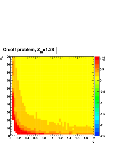
Figure 1: For the on/off problem analyzed using the $Z_{\rm Bi}$ recipe, for each fixed value of $\tau$ and $\mu_{\rm b}$, the plot indicates the calculated $Z_{\rm true}-Z_{\rm claim}$ for the ensemble of experiments quoting a $Z_{\rm claim}\geq 1.28$, i.e., a $p$-value of 0.1 or smaller.

For the on/off experiments analyzed using the $Z_{\rm Bi}$ recipe, the results are displayed in Figs. 1 through 3. Each plot corresponds to a particular value of $Z_{\rm claim}$, and for each point $(\tau,\mu_{\rm b})$ chosen on a fine grid of 50 by 50 points $Z_{\rm true}-Z_{\rm claim}$ is indicated. As with all these figures, the right plot is a zoomed-in version of the left. The value indicated in each pixel is calculated using the $(\tau,\mu_{\rm b})$ of its lower left corner. As expected from the construction, $Z_{\rm true}\geq Z_{\rm claim}$ everywhere; the overcoverage is significant for small values of counts, where the discreteness is most relevant, as seen in the lower left corner of the zoomed-in version of each figure. This overcoverage could be reduced by using the non-standard intervals for the ratio of Poisson means in Ref. [22], but we do not pursue that option in this paper.

At the limit of numerical precision in our implementation, it turns out that the result errs in the conservative direction, but of course extreme caution should be used to avoid quoting a result badly affected in this way. The highest calculated value of $Z_{\rm true}$ is nearly 7.6 (corresponding to a $p$-value of $\sim 10^{-14}$) due to the machine limit of our implementation of the calculation of $Z_{\rm true}$ from the $p$-value; this can be alleviated by using approximation in Eqn. 4, but we do not pursue that option in this paper, and leave blank those regions in the plot where the associated $p$-value is less than $\sim 10^{-14}$.

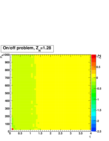
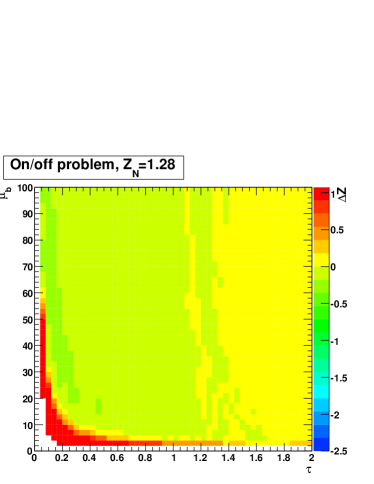
Figure 4: For the on/off problem analyzed using the $Z_{\rm N}$ recipe, for each fixed value of $\tau$ and $\mu_{\rm b}$, the plot indicates the calculated $Z_{\rm true}-Z_{\rm claim}$ for the ensemble of experiments quoting $Z_{\rm claim}\geq 1.28$, i.e., a $p$-value of $0.1$ or smaller.

When using the $Z_{\rm N}$ recipe to analyze the on/off experiments (Figs. 4 through 6), there is a large region in which the method undercovers (by as much as two units of $Z$ at very low $\tau$) with the extent of the region depending on $Z_{\rm claim}$. This is in accord with Cranmer [12], who, using the Monte Carlo method, finds for a specific case ($\mu_{\rm b}=$100, $\tau=$1), that the $Z_{\rm N}$ recipe undercovers for $Z_{\rm claim}=5$, with a Type I error rate corresponding to $Z_{\rm true}=4.2$. Again, there is overcoverage due to discreteness at small values of $\mu_{\rm b}$ and $\tau$.

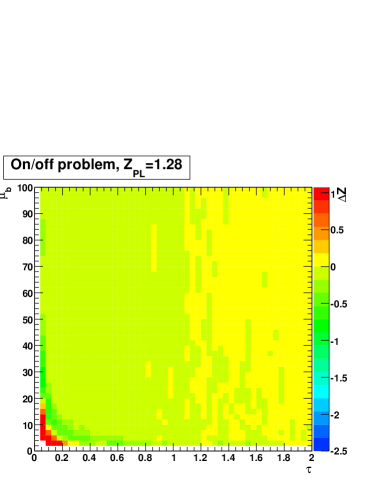
Figure 7: For the on/off problem analyzed using the profile likelihood method, for each fixed value of $\tau$ and $\mu_{\rm b}$, the plot indicates the calculated $Z_{\rm true}-Z_{\rm claim}$ for the ensemble of experiments quoting $Z_{\rm claim}\geq 1.28$, i.e., a $p$-value of $0.1$ or smaller.

The results of using the profile likelihood method to analyze the on/off experiments are shown in Figs. 7 through 9. There is slight undercoverage over much of the parameter space, by at most half a unit of $Z$ or so. As the true parameters $\mu_{\rm b}$ and $\tau$ move away from the origin, initially there is overcoverage caused by discreteness, giving way to the region of largest undercoverage for $Z_{\rm PL}$, which then becomes only slight undercoverage as near-asymptotic performance is reached. At the point considered by Cranmer [12] of $\mu_{\rm b}=$100, $\tau=$1, we calculate $Z_{\rm true}=4.99$, in good agreement with the result from his MC method of $Z_{\rm true}=5.0$. For small $\mu_{\rm b}$ and large $\tau$ (with the qualifiers small and large becoming stricter for increasing $Z_{\rm claim}$), the nominal coverage is achieved.

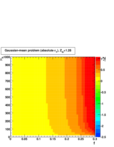
Figure 10: For the Gaussian-mean background problem with exactly known $\sigma_{\rm b}$, analyzed using the $Z_{\rm Bi}$ recipe, for each fixed value of $f=\sigma_{\rm b}/\mu_{\rm b}$ and $\mu_{\rm b}$, the plot indicates the calculated $Z_{\rm true}-Z_{\rm claim}$ for the ensemble of experiments quoting $Z_{\rm claim}\geq 1.28$, i.e., a $p$-value of $0.1$ or smaller.

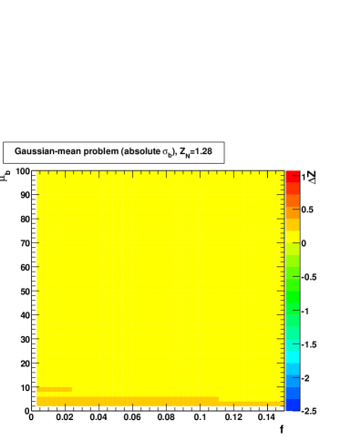
Figure 13: For the Gaussian-mean background problem with exactly known $\sigma_{\rm b}$, analyzed using the $Z_{\rm N}$ recipe, for each fixed value of $f=\sigma_{\rm b}/\mu_{\rm b}$ and $\mu_{\rm b}$, the plot indicates the calculated $Z_{\rm true}-Z_{\rm claim}$ for the ensemble of experiments quoting $Z_{\rm claim}\geq 1.28$, i.e., a $p$-value of $0.1$ or smaller.

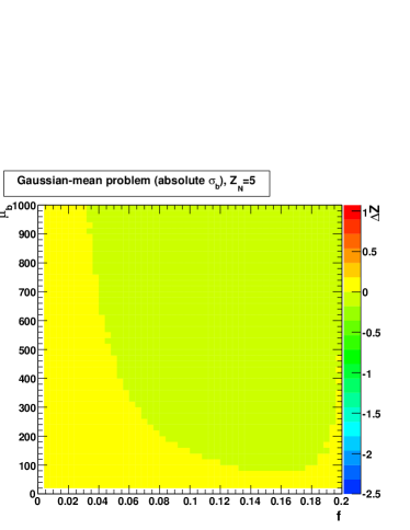
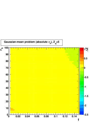
Figure 15: For the Gaussian-mean background problem with exactly known $\sigma_{\rm b}$, analyzed using the $Z_{\rm N}$ recipe, for each fixed value of $f=\sigma_{\rm b}/\mu_{\rm b}$ and $\mu_{\rm b}$, the plot indicates the calculated $Z_{\rm true}-Z_{\rm claim}$ for the ensemble of experiments quoting $Z_{\rm claim}\geq 5$, i.e., a $p$-value of $2.87\times 10^{-7}$ or smaller.

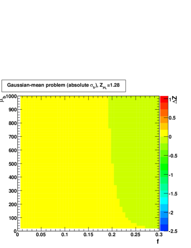
Figure 16: For the Gaussian-mean background problem with exactly known $\sigma_{\rm b}$, analyzed using the profile likelihood method, for each fixed value of $f=\sigma_{\rm b}/\mu_{\rm b}$ and $\mu_{\rm b}$, the plot indicates the calculated $Z_{\rm true}-Z_{\rm claim}$ for the ensemble of experiments quoting $Z_{\rm claim}\geq 1.28$, i.e., a $p$-value of $0.1$ or smaller.

For the Gaussian-mean background problem with exactly known $\sigma_{\rm b}$, the results are in Figs. 10 through 12 when analyzed with $Z_{\rm Bi}$; in Figs. 13 through 15 when analyzed with $Z_{\rm N}$; and in Figs. 16 through 18 when analyzed with $Z_{\rm PL}$. $Z_{\rm Bi}$ overcovers everywhere, quite severely for the larger values of $f$ considered; this is an effect of small estimates of $\hat{\mu}_{\rm b}$ leading by the rough correspondence of Eqn. 8 to underestimates of the shape-controlling parameter $\tau=\hat{\mu}_{\rm b}/\sigma_{\rm b}^{2}$, and thus to an overly broad and shifted gamma distribution which in turn leads to estimated tail probabilities which are inappropriately large. $Z_{\rm N}$ provides slight over-coverage and no undercoverage for $Z_{\rm claim}=1.28$ and $Z_{\rm claim}=3$, but it undercovers for for $Z_{\rm claim}=5$ at larger values of $f$ and $\mu_{\rm b}$. For the largest values of $f$ in Fig. 15, the reduction in undercoverage is an artifact of using the truncated Gaussian model for the uncertainty in the mean background, as the condition of Eqn. 18 comes into play. $Z_{\rm PL}$ has good coverage over the entire parameter space shown, with some effect of discreteness observable.

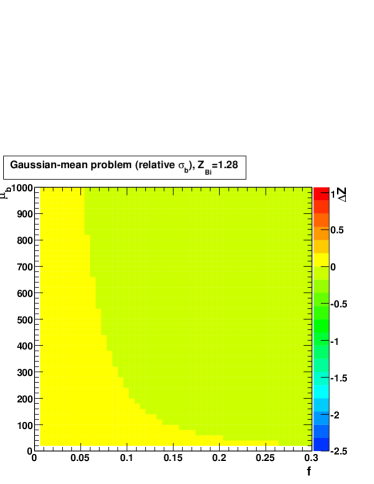
Figure 19: For the Gaussian-mean background problem with exactly known relative uncertainty $f$, analyzed using the $Z_{\rm Bi}$ recipe, for each fixed value of $f$ and $\mu_{\rm b}$, the plot indicates the calculated $Z_{\rm true}-Z_{\rm claim}$ for the ensemble of experiments quoting $Z_{\rm claim}\geq 1.28$, i.e., a $p$-value of $0.1$ or smaller.

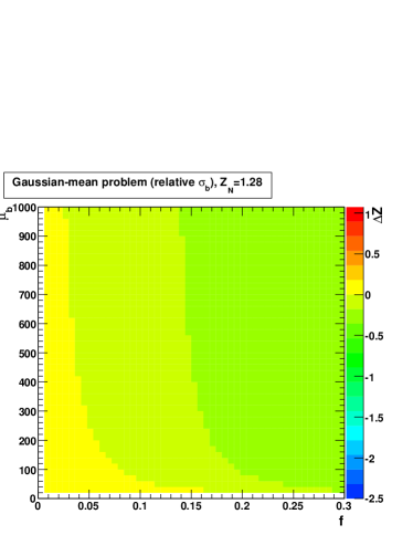
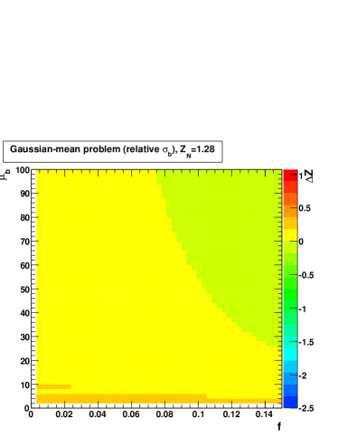
Figure 22: For the Gaussian-mean background problem with exactly known relative uncertainty $f$, analyzed using the $Z_{\rm N}$ recipe, for each fixed value of $f$ and $\mu_{\rm b}$, the plot indicates the calculated $Z_{\rm true}-Z_{\rm claim}$ for the ensemble of experiments quoting $Z_{\rm claim}\geq 1.28$, i.e., a $p$-value of $0.1$ or smaller.

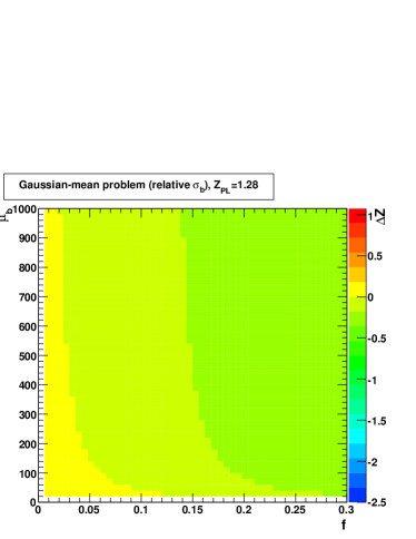
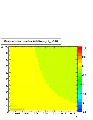
Figure 25: For the Gaussian-mean background problem with exactly known relative uncertainty $f$, analyzed using the profile likelihood method, for each fixed value of $f$ and $\mu_{\rm b}$, the plot indicates the calculated $Z_{\rm true}-Z_{\rm claim}$ for the ensemble of experiments quoting $Z_{\rm claim}\geq 1.28$, i.e., a $p$-value of $0.1$ or smaller.

For the Gaussian-mean background problem with exactly known relative uncertainty $f$, the results are in Figs. 19 through 21 when analyzed with $Z_{\rm Bi}$; in Figs. 22 through 24 when analyzed with $Z_{\rm N}$; and in Figs. 25 through 27 when analyzed with $Z_{\rm PL}$. Both $Z_{\rm Bi}$ and $Z_{\rm N}$ give good coverage for small values of $f$ and small $\mu_{\rm b}$, but both undercover for large regions of the parameter space, with $Z_{\rm Bi}$ performing slightly better in some regions. The undercoverage of $Z_{\rm Bi}$ is an effect of small estimates of $\hat{\mu}_{\rm b}$ leading by the rough correspondence of Eqn. 8 to overestimates of the shape-controlling $\tau=1/(f^{2}\hat{\mu}_{\rm b})$, and thus to an overly narrow gamma distribution, which in turn leads to estimated tail probabilities which are inappropriately small. For $Z_{\rm PL}$, the region of good coverage is smaller in $\mu_{\rm b}$ and $f$ than for either of $Z_{\rm Bi}$ or $Z_{\rm N}$, but like the latter two, the profile likelihood method also undercovers for a large part of the parameter space for this problem.

In all of the results shown for $Z_{\rm PL}$ for the Gaussian-mean background problem (Figs. 16 through 18 and Figs. 25 through 27), we assume (as we believe to be common practice) that the experimenter is truncating the Gaussian pdf for $\hat{\mu}_{\rm b}$ at zero, i.e., set $P(\hat{\mu}_{\rm b}|\mu_{\rm b})=0$ for $\hat{\mu}_{\rm b}\leq 0$ and renormalized. This results in a denominator for ${\cal L}_{\rm G}$ which depends on $\mu_{\rm b}$, and the determination of $Z_{\rm PL}$ is performed numerically. As with the discussion of Gaussian truncation above for $p(\mu_{\rm b})$, if this ad hoc procedure makes any material difference, one should explore other functional forms. As a check, we removed the truncation, i.e., used Eqn. 21 as it is written. The only perceptible difference is in Figs. 16 through 18, where the slight undercoverage at $f>0.1$ disappears.

10 Conclusion

As seen in these simple prototype problems, naive use of a recipe for including systematic errors can lead to significant departure from the claimed $Z$. For a true on/off problem (sideband estimate of background in a binned analysis), $Z_{\rm Bi}=Z_{\Gamma}$ avoids undercoverage by construction, but can be quite conservative for small numbers of events, at least when the standard intervals for ratio of Poisson means are used. Since undercoverage is usually considered to be worse than overcoverage, we recommend $Z_{\rm Bi}$ be considered for general use in this problem; for a range of values, it is conveniently implemented in ROOT, as illustrated in Appendix E. However, one should be aware of the overcoverage with small numbers of events, and perhaps consider use of alternative intervals for the binomial parameter or the ratio of Poisson means. Consistent with long experience in HEP and GRA and as noted by Rolke et al. [9, 10], the profile likelihood-derived $Z_{\rm PL}$ provides a strikingly good approximation in most of the parameter space, with at most modest under-coverage; thus $Z_{\rm PL}$ should also be routinely calculated, especially given the easy use of the formula of Li and Ma, Eqn. 25.

For the Gaussian-mean background problem, $Z_{\rm Bi}$ works as well as or better than $Z_{\rm N}$ in much of the space; for extremely small uncertainties on a large mean background, the implementation in ROOT can be supplemented using Ref. [21]. The profile likelihood method performs extremely well for exactly known $\sigma_{\rm b}$ For the case of exactly known relative $f$, all three methods have severe under-coverage for high values of $Z_{\rm claim}$ and $f>0.1$. Since $Z_{\rm Bi}$ and $Z_{\rm N}$ are not well-founded for the Gaussian-mean background problem, and since the profile likelihood is based on asymptotic theory, checks of coverage in the region of application are essential.

This paper explores only three recipes for two simple problems; of course, it is of interest to extend the studies to other recipes and more complex problems. For example, if the background in the signal region has several components, each estimated in a separate subsidiary experiment, one can attempt to summarize this information approximately and apply single-components methods. (One could try both an approximate $Z_{\rm N}$ and a scaled $Z_{\Gamma}$ where the scaling reflects the ratio $f=\sigma_{\rm b}/\mu_{\rm b}$.) $Z_{\rm PL}$ can be extended to likelihood functions describing all components. As problems become more complex, exact coverage by construction is not likely to be achieved, since even when a full-blown Neyman construction is feasible (guaranteeing no undercoverage), it typically leads to overcoverage. When approximations such as combining background components are made, one should check the coverage with a full simulation reflecting the individual components.

As Monte Carlo simulation or numerical integration is often used even for the simplest problems, the fact the $Z_{\rm PL}$ has the simple expression in Eqn. 25 is extremely useful both for checking the results of a simulation, or for providing a speedy evaluation (e.g. in GRA when data from many segments of the sky must be monitored in real time). While for some parameters evaluation of $Z_{\rm Bi}$ encounters numerical problems, its expression in terms of the incomplete beta function is also quite convenient.

All of these issues become even more severe as $Z$ values as high as 5 or even higher are sought or quoted, as is common in high energy physics. The implied tail probability of $2.87\times 10^{-7}$ should be used with caution, as it can be extremely sensitive to underlying assumptions. While this paper explores the coverage assuming that the model is correct, for high $Z$ values one is of course also susceptible to modeling errors, for example non-Gaussian tails in the uncertainties.

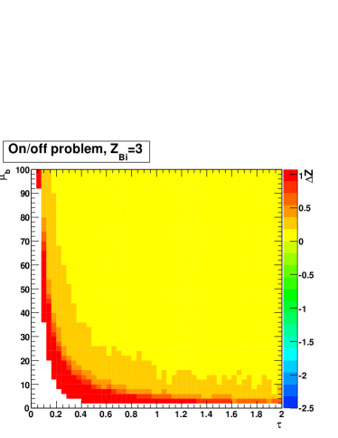
Figure 2: For the on/off problem analyzed using the $Z_{\rm Bi}$ recipe, for each fixed value of $\tau$ and $\mu_{\rm b}$, the plot indicates the calculated $Z_{\rm true}-Z_{\rm claim}$ for the ensemble of experiments quoting $Z_{\rm claim}\geq 3$, i.e., a $p$-value of $1.35\times 10^{-3}$ or smaller.

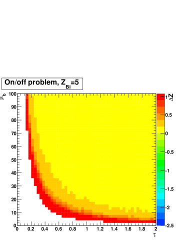
Figure 3: For the on/off problem analyzed using the $Z_{\rm Bi}$ recipe, for each fixed value of $\tau$ and $\mu_{\rm b}$, the plot indicates the calculated $Z_{\rm true}-Z_{\rm claim}$ for the ensemble of experiments quoting $Z_{\rm claim}\geq 5$, i.e., a $p$-value of $2.87\times 10^{-7}$ or smaller.

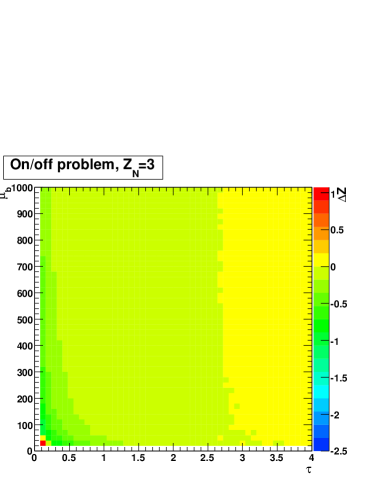
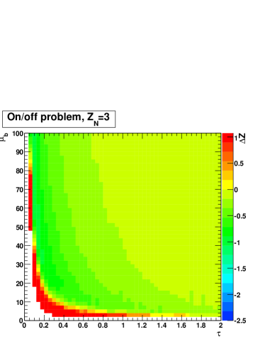
Figure 5: For the on/off problem analyzed using the $Z_{\rm N}$ recipe, for each fixed value of $\tau$ and $\mu_{\rm b}$, the plot indicates the calculated $Z_{\rm true}-Z_{\rm claim}$ for the ensemble of experiments quoting $Z_{\rm claim}\geq 3$, i.e., a $p$-value of $1.35\times 10^{-3}$ or smaller.

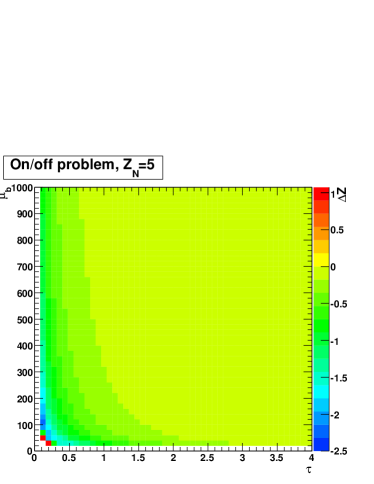
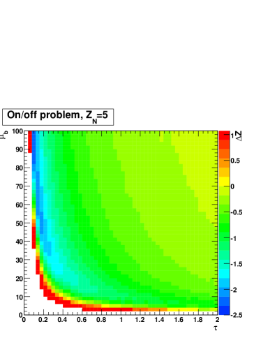
Figure 6: For the on/off problem analyzed using the $Z_{\rm N}$ recipe, for each fixed value of $\tau$ and $\mu_{\rm b}$, the plot indicates the calculated $Z_{\rm true}-Z_{\rm claim}$ for the ensemble of experiments quoting $Z_{\rm claim}\geq 5$, i.e., a $p$-value of $2.87\times 10^{-7}$ or smaller.

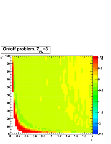
Figure 8: For the on/off problem analyzed using the profile likelihood method, for each fixed value of $\tau$ and $\mu_{\rm b}$, the plot indicates the calculated $Z_{\rm true}-Z_{\rm claim}$ for the ensemble of experiments quoting $Z_{\rm claim}\geq 3$, i.e., a $p$-value of $1.35\times 10^{-3}$ or smaller.

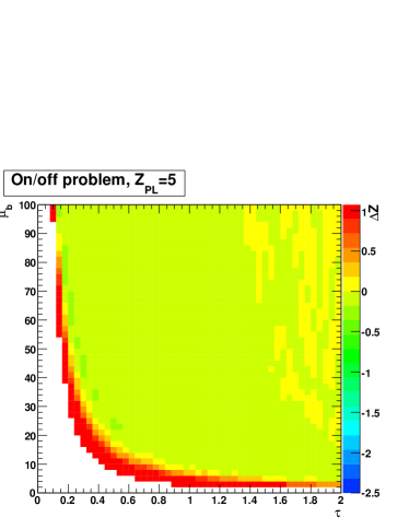
Figure 9: For the on/off problem analyzed using the profile likelihood method, for each fixed value of $\tau$ and $\mu_{\rm b}$, the plot indicates the calculated $Z_{\rm true}-Z_{\rm claim}$ for the ensemble of experiments quoting $Z_{\rm claim}\geq 5$, i.e., a $p$-value of $2.87\times 10^{-7}$ or smaller.

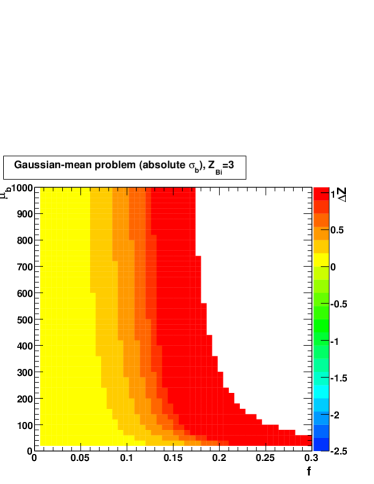
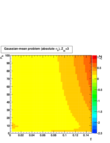
Figure 11: For the Gaussian-mean background problem with exactly known $\sigma_{\rm b}$, analyzed using the $Z_{\rm Bi}$ recipe, for each fixed value of $f=\sigma_{\rm b}/\mu_{\rm b}$ and $\mu_{\rm b}$, the plot indicates the calculated $Z_{\rm true}-Z_{\rm claim}$ for the ensemble of experiments quoting $Z_{\rm claim}\geq 3$, i.e., a $p$-value of $1.35\times 10^{-3}$ or smaller.

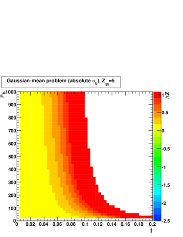
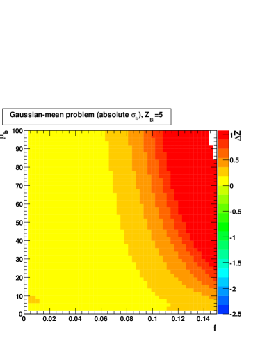
Figure 12: For the Gaussian-mean background problem with exactly known $\sigma_{\rm b}$, analyzed using the $Z_{\rm Bi}$ recipe, for each fixed value of $f=\sigma_{\rm b}/\mu_{\rm b}$ and $\mu_{\rm b}$, the plot indicates the calculated $Z_{\rm true}-Z_{\rm claim}$ for the ensemble of experiments quoting $Z_{\rm claim}\geq 5$, i.e., a $p$-value of $2.87\times 10^{-7}$ or smaller.

Figure 14: For the Gaussian-mean background problem with exactly known $\sigma_{\rm b}$, analyzed using the $Z_{\rm N}$ recipe, for each fixed value of $f=\sigma_{\rm b}/\mu_{\rm b}$ and $\mu_{\rm b}$, the plot indicates the calculated $Z_{\rm true}-Z_{\rm claim}$ for the ensemble of experiments quoting $Z_{\rm claim}\geq 3$, i.e., a $p$-value of $1.35\times 10^{-3}$ or smaller.

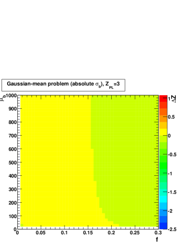
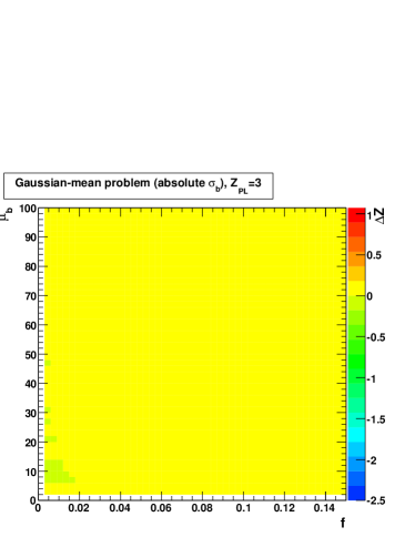
Figure 17: For the Gaussian-mean background problem with exactly known $\sigma_{\rm b}$, analyzed using the profile likelihood method, for each fixed value of $f=\sigma_{\rm b}/\mu_{\rm b}$ and $\mu_{\rm b}$, the plot indicates the calculated $Z_{\rm true}-Z_{\rm claim}$ for the ensemble of experiments quoting $Z_{\rm claim}\geq 3$, i.e., a $p$-value of $1.35\times 10^{-3}$ or smaller.

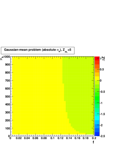
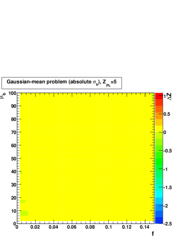
Figure 18: For the Gaussian-mean background problem with exactly known $\sigma_{\rm b}$, analyzed using the profile likelihood method, for each fixed value of $f=\sigma_{\rm b}/\mu_{\rm b}$ and $\mu_{\rm b}$, the plot indicates the calculated $Z_{\rm true}-Z_{\rm claim}$ for the ensemble of experiments quoting $Z_{\rm claim}\geq 5$, i.e., a $p$-value of $2.87\times 10^{-7}$ or smaller.

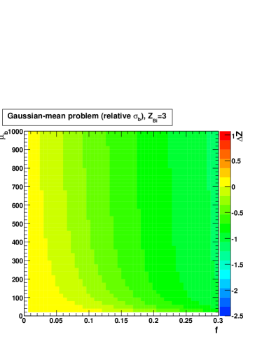
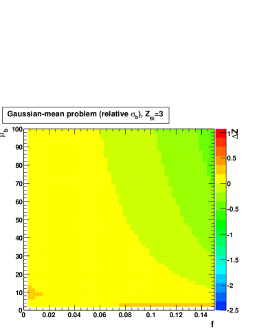
Figure 20: For the Gaussian-mean background problem with exactly known relative uncertainty $f$, analyzed using the $Z_{\rm Bi}$ recipe, for each fixed value of $f$ and $\mu_{\rm b}$, the plot indicates the calculated $Z_{\rm true}-Z_{\rm claim}$ for the ensemble of experiments quoting $Z_{\rm claim}\geq 3$, i.e., a $p$-value of $1.35\times 10^{-3}$ or smaller.

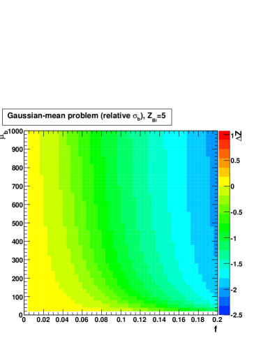
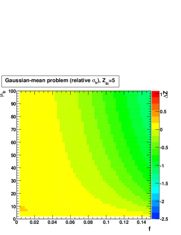
Figure 21: For the Gaussian-mean background problem with exactly known relative uncertainty $f$, analyzed using the $Z_{\rm Bi}$ recipe, for each fixed value of $f$ and $\mu_{\rm b}$, the plot indicates the calculated $Z_{\rm true}-Z_{\rm claim}$ for the ensemble of experiments quoting $Z_{\rm claim}\geq 5$, i.e., a $p$-value of $2.87\times 10^{-7}$ or smaller.

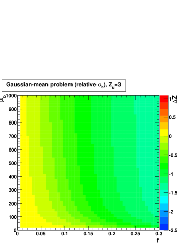
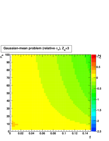
Figure 23: For the Gaussian-mean background problem with exactly known relative uncertainty $f$, analyzed using the $Z_{\rm N}$ recipe, for each fixed value of $f$ and $\mu_{\rm b}$, the plot indicates the calculated $Z_{\rm true}-Z_{\rm claim}$ for the ensemble of experiments quoting $Z_{\rm claim}\geq 3$, i.e., a $p$-value of $1.35\times 10^{-3}$ or smaller.

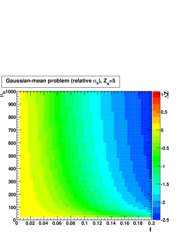
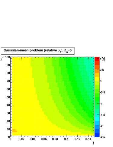
Figure 24: For the Gaussian-mean background problem with exactly known relative uncertainty $f$, analyzed using the $Z_{\rm N}$ recipe, for each fixed value of $f$ and $\mu_{\rm b}$, the plot indicates the calculated $Z_{\rm true}-Z_{\rm claim}$ for the ensemble of experiments quoting $Z_{\rm claim}\geq 5$, i.e., a $p$-value of $2.87\times 10^{-7}$ or smaller.

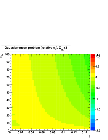
Figure 26: For the Gaussian-mean background problem with exactly known relative uncertainty $f$, analyzed using the profile likelihood method, for each fixed value of $f$ and $\mu_{\rm b}$, the plot indicates the calculated $Z_{\rm true}-Z_{\rm claim}$ for the ensemble of experiments quoting $Z_{\rm claim}\geq 3$, i.e., a $p$-value of $1.35\times 10^{-3}$ or smaller.

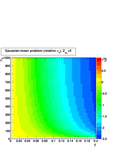
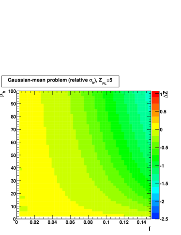
Figure 27: For the Gaussian-mean background problem with exactly known relative uncertainty $f$, analyzed using the profile likelihood method, for each fixed value of $f$ and $\mu_{\rm b}$, the plot indicates the calculated $Z_{\rm true}-Z_{\rm claim}$ for the ensemble of experiments quoting $Z_{\rm claim}\geq 5$, i.e., a $p$-value of $2.87\times 10^{-7}$ or smaller.

Appendix A Notation

Table 2 defines the variables used in this paper.

Table 2:

Symbol	definition
$n_{\rm off}$	total observed in “off” (background) region
$n_{\rm on}$	total observed in “on” (signal) region
$n_{\rm tot}$	$n_{\rm on}+n_{\rm off}$
$\mu_{\rm s}$	true signal mean in “on” (signal) region
$\mu_{\rm b}$	true background mean in “on” (signal) region
$\hat{\mu}_{\rm b}$	estimate of background mean in “on” (signal) region
$\sigma_{\rm b}$	uncertainty on estimate $\hat{\mu}_{\rm b}$ in “on” region
$s$	estimate of signal events in the “on” region = $n_{\rm on}-\hat{\mu}_{\rm b}$
$f$	relative uncertainty on $\hat{\mu}_{\rm b}$; $\sigma_{\rm b}/\mu_{b}$
$\mu_{\rm on}$	true total mean in signal region = $\mu_{s}+\mu_{b}$
$\mu_{\rm off}$	true background mean in “off” (background) region
$\mu_{\rm tot}$	true total mean in “on” plus “off” regions = $\mu_{\rm on}+\mu_{\rm off}$
$\tau$	ratio of background means in “off” and “on” regions: $\mu_{\rm off}/\mu_{\rm b}$
$\lambda$	ratio of Poisson means $\mu_{\rm off}/\mu_{\rm on}$
$\rho$	binomial parameter $\mu_{\rm on}/\mu_{\rm tot}$

Appendix B Derivation of approximate tail area of normal distribution

With $\Phi(Z)=1-p$ defined in Eqns. 1-2, we derive Eqn. 4 by starting with the large-$Z$ expansion of $1-\Phi(Z)$, the cumulative distribution of the normal density $\phi(Z)$, given as asymptotic expansion 26.2.12 in Ref. [49]:

$$p=1-\Phi(Z)\approx\frac{\phi(Z)}{Z}\ (1-\frac{1}{Z^{2}}+\dots)$$ (33)

Then we follow Ref. [5] by neglecting the higher order terms,

$$p=\frac{1}{\sqrt{2\pi}}\frac{\exp(-Z^{2}/2)}{Z},$$ (34)

$$\ln(p\sqrt{2\pi})=-Z^{2}/2-\ln Z.$$ (35)

Defining $u$ by further manipulation of the left side,

$$u=-2\ln(p\sqrt{2\pi})=Z^{2}+\ln Z^{2},$$ (36)

and substituting $Z^{2}\approx u$ into $\ln Z^{2}$ by initially neglecting this term, we obtain

$$Z^{2}=u-\ln Z^{2}\approx u-\ln u.$$ (37)

Thus

$$Z\approx\sqrt{u-\ln u}.$$ (38)

Appendix C Proof of the identity of $Z_{\rm Bi}$ and $Z_{\Gamma}$

The essence of the proof is to tie together two established identities. The first is a “parameter mixing” [27, 50] identity that relates the negative binomial distribution to a mix of Poisson distributions with mean drawn from a Gamma density (as found in $p_{\Gamma}$); the second connects binomial tail probabilities (as found in $p_{\rm Bi}$) to negative binomial tail probabilities.

We start by combining Eqns. 15, 17, and 19, arriving at the expression (equivalent to Eqn. 6 of Ref. [32], also in Sec. III of Ref. [5]), using $\alpha=1/\tau$,

$$p_{\Gamma}=\sum_{j=n_{\rm on}}^{\infty}\frac{\alpha^{j}(1/(1+\alpha))^{1+j+n_{\rm off}}(j+n_{\rm off})!}{j!\,n_{\rm off}!}.$$ (39)

Substituting for $\alpha$ in terms of $\rho=1/(1+\tau)=\alpha/(1+\alpha)$:

$$p_{\Gamma}=\sum_{j=n_{\rm on}}^{\infty}\frac{\rho^{j}(1-\rho)^{1+n_{\rm off}}(j+n_{\rm off})!}{j!\,n_{\rm off}!}$$ (40)

$$=\sum_{j=n_{\rm on}}^{\infty}{\rm NBi}(N_{\rm on}=j;\,N_{\rm off}=n_{\rm off}+1,\,{\rm prob_{\rm success}=1-\rho}).$$ (41)

As indicated, the term summed can be identified as the negative binomial [27, 50] probability NBi for observing $j$ counts on-source (confusingly corresponding to number of “failures” in the usual exposition of NBi) in less time than it takes to observe exactly $n_{\rm off}+1$ counts off-source (number of “successes” $N_{\rm off}$), where as above, $\rho=\mu_{\rm on}/\mu_{\rm tot}$ is the ratio of the mean numbers of counts on-source to the total mean on and off source (and hence $1-\rho$ corresponds to the usual probability for “success” in NBi). Thus, in more compact notation,

$$p_{\Gamma}={\rm NBi}(N_{\rm on}>n_{\rm on}-1|N_{\rm off}=n_{\rm off}+1),$$ (42)

thus completing the first main identity.

Now the probability for more than $k$ on-source counts while waiting for $m$ off-source counts is precisely equal [27] to the probability of finding fewer than $m$ off-source counts in exactly $k+m$ total counts for the same ratio of (on/total) means $\rho$. This relates a negative binomial tail probability to the (ordinary) binomial tail probability:

$${\rm NBi}(N_{\rm on}>k|N_{\rm off}=m)={\rm Bi}(N_{\rm off}<m|k+m).$$ (43)

The left hand side of this identify matches the right hand side of Eqn. 42 for $k=n_{\rm on}-1$ and $m=n_{\rm off}+1$, so Eqn. 42 becomes

$$p_{\Gamma}={\rm Bi}(N_{\rm off}<n_{\rm off}+1|n_{\rm on}+n_{\rm off})={\rm Bi}(N_{\rm off}<n_{\rm off}+1|n_{\rm tot}).$$ (44)

Since the sum of counts is constrained in the Binomial probability, the latter expression can be re-written in terms of complementary outcomes:

$$p_{\Gamma}={\rm Bi}(N_{\rm on}\geq n_{\rm on}|n_{\rm tot}).$$ (45)

Comparing with Eqn. 13 confirms that $p_{\rm Bi}=p_{\Gamma}$ and hence $Z_{\rm Bi}=Z_{\Gamma}$. This relation was first proved by other methods in 2003 [34], but the present proof seems to be more illuminating.

Appendix D Details of the Calculations of $Z_{\rm true}$

This Appendix provides more details of the calculation of $Z_{\rm true}$ in Sec. 9.

D.1 Details of calculation of $Z_{\rm true}$ for the on/off problem

For each point in $(\mu_{\rm b},\tau)$ space for which one calculates $Z_{\rm true}$, one has a plane of discrete points $(n_{\rm off},n_{\rm on})$, with each point having the joint probability $P(n_{\rm on}|\mu_{\rm b})\cdot P(n_{\rm off}|\tau\mu_{\rm b})$, where $P$ is the Poisson probability. The joint probabilities of all the points $(n_{\rm off},n_{\rm on})$ for which the recipe studied returns $Z\geq Z_{\rm claim}$ are summed to obtain the Type I error rate for a test with the implied significance level. Navigating in the plane of $(n_{\rm off},n_{\rm on})$ is facilitated making use of Eqn. 10 and thus considering lines of constant $n_{\rm tot}$, along which binomial probabilities are calculated to obtain efficiently the contour bounding the region with $Z\geq Z_{\rm claim}$.

D.1.1 The $Z_{\rm Bi}$ recipe applied to the on/off problem

In this simplest case, $\tau$ is fixed and given, so for each $(n_{\rm off},n_{\rm on})$ point, $p_{\rm Bi}$ and $Z_{\rm Bi}$ are calculated from Eqns. 14 and 3, and compared to $Z_{\rm claim}$.

D.1.2 The $Z_{\rm N}$ recipe applied to the on/off problem

Starting with $n_{\rm on}$, $n_{\rm off}$, and $\tau$, one obtains $\hat{\mu}_{\rm b}$ from Eqn. 6), $\sigma_{\rm b}$ from Eqn. 7, and proceeds as usual. ($f$ is thereby equal to $1/\sqrt{n_{\rm off}}$.)

D.1.3 The profile likelihood method applied to the on/off problem

We proceed exactly as in Sec. D.1.1, but instead of calculating a $p$-value and then $Z$ at each point $(n_{\rm off},n_{\rm on})$, $Z$ is calculated directly from Eqn. 24.

D.2 Details of calculation of $Z_{\rm true}$ for the Gaussian-mean background problem

For each point in $(f,\mu_{\rm b})$ space for which one calculates $Z_{\rm true}$ corresponding to a particular $Z_{\rm claim}$, one considers all values of $n_{\rm on}$, and for each value of $n_{\rm on}$ one finds (via a binary search) the critical value of $\hat{\mu}_{\rm b}$ such that $Z=Z_{\rm claim}$. Then the Type I error rate is the sum of the products of the probability of obtaining each $n_{\rm on}$ and the Gaussian tail probability for $\hat{\mu}_{\rm b}$ such that $Z\geq Z_{\rm claim}$ for that $n_{\rm on}$. The tail probability is obtained using the error function and true values of $\mu_{\rm b}$ and $\sigma_{\rm b}=f\mu_{\rm b}$.

D.2.1 The $Z_{\rm N}$ recipe applied to the Gaussian-mean background problem

In the case where $\sigma_{\rm b}$ is assumed known, $Z_{\rm N}$ is directly computed; in the case where $f$ is known, $\sigma_{\rm b}$ is first estimated by $f\hat{\mu}_{\rm b}$.

D.2.2 The $Z_{\rm Bi}$ recipe applied to the Gaussian-mean background problem

This again uses the rough correspondence of Eqn. 8. In the case where $\sigma_{\rm b}$ is known exactly, then for each $n_{\rm on}$, one searches for $\hat{\mu}_{\rm b}$ such that when $\hat{\mu}_{\rm b}$ is used in Eqns. 8 and 6 to obtain $\tau$ and $n_{\rm off}$, the resulting $Z_{\rm Bi}$ from Eqns. 14 and 3 is equal to $Z_{\rm claim}$. In the case where $f$ is known exactly, as usual one first estimates $\sigma_{\rm b}$ by $f\hat{\mu}_{\rm b}$ and then in the same way finds the critical value of $\hat{\mu}_{\rm b}$. (I.e., one computes $\tau=\hat{\mu}_{\rm b}/(f\hat{\mu}_{\rm b})^{2}$ and $n_{\rm off}=\hat{\mu}_{\rm b}\tau$, from which one obtains $Z_{\rm Bi}$.)

D.2.3 The profile likelihood method applied to the Gaussian-mean background problem

Once more using the rough correspondence of Eqn. 8, we search for the $\hat{\mu}_{\rm b}$ such that when calculating $\tau$ and $n_{\rm off}$ as in Sec. D.2.2, the resulting $Z$ using Eqn. 24 is equal to $Z_{\rm claim}$.

Appendix E Implementation of $Z_{\rm Bi}$ in ROOT

As noted in Sec. 3, the ratio in Eqn. 14 is implemented in ROOT [20] following the algorithm in Numerical Recipes [19]; therefore one simply calls BetaIncomplete to obtain the $p$-value, and then ErfInverse to convert it to $Z$ according to Eqn. 3.

For the simple on/off problem with $n_{\rm on}=140$, $n_{\rm off}=100$, and $\tau=1.2$, the ROOT commands are:

double n_on = 140.
double n_off = 100.
double tau = 1.2
double P_Bi = TMath::BetaIncomplete(1./(1.+tau),n_on,n_off+1)
double Z_Bi = sqrt(2)*TMath::ErfInverse(1 - 2*P_Bi)

yielding $p_{\rm Bi}=4.19\times 10^{-5}$ and $Z_{\rm Bi}=3.93$.

In order to apply $Z_{\rm Bi}$ to the Gaussian-mean background problem, consider for example the observations $n_{\rm on}=140$ and $\hat{\mu}_{\rm b}=83.3\pm 8.33$. Using the correspondence in Eqn. 8 to obtain $\tau$, and then Eqn. 6 to obtain $n_{\rm off}=\hat{\mu}_{\rm b}\,\tau$, the ROOT commands are similarly

double n_on = 140.
double mu_b_hat = 83.33
double sigma_b = 8.333
double tau = mu_b_hat/(sigma_b*sigma_b)
double n_off = tau*mu_b_hat
double P_Bi = TMath::BetaIncomplete(1./(1.+tau),n_on,n_off+1)
double Z_Bi = sqrt(2)*TMath::ErfInverse(1 - 2*P_Bi)

The result in this example is then identical to the on/off example within round-off error, since the chosen $\hat{\mu}_{\rm b}$ and $\sigma_{\rm b}$ were chosen to reproduce the same $\tau$ and $n_{\rm off}$.

As $\sigma_{\rm b}$ becomes small, $\tau$ and $n_{\rm off}$ become large, so ironically this implementation encounters numerical trouble for small uncertainty on the background (and in particular background known exactly). For such small errors on background, neglecting them using Eqn. 15 seems reasonable but should be studied further. The implementation of the incomplete beta function by Majumder and Bhattacharjee [21] used for the coverage calculations in Sec. 3 provides some expanded capability. Beyond that, one may consider using the asymptotic formulas in Eqn. 4.

References

- [1] For a recent review, see Robert D. Cousins, “Treatment of Nuisance Parameters in High Energy Physics, and Possible Justifications and Improvements in the Statistics Literature”, Proceedings of PhyStat 05: Statistical Problems in Particle Physics, Astrophysics and Cosmology (Oxford, Sept. 12-15, 2005), http://www.physics.ox.ac.uk/phystat05/proceedings/. See also the response following by N. Reid.
- [2] For a comprehensive discussion of hypothesis testing, see A. Stuart, K. Ord, and S. Arnold, Kendall’s Advanced Theory of Statistics, Volume 2A, 6th ed., (London:Arnold, 1999), and earlier editions by Kendall and Stuart. From the formal correspondence between hypothesis tests and confidence intervals in Chapter 20, all the frequentist hypothesis tests in this paper can be restated in terms of confidence intervals and limits.
- [3] J.O. Berger, T. Sellke “Testing a Point Null Hypothesis: The Irreconcilability of Values and Evidence”, JASA 82, 112 (1987)
- [4] T. Sellke, M.J. Bayarri, J.O. Berger “Calibration of p values for Testing Precise Null Hypotheses” Amer. Statistician 55, 62 (2001)
- [5] James T. Linnemann, “Measures of significance in HEP and astrophysics,” Proceedings of PhyStat 2003: Statistical Problems in Particle Physics, Astrophysics, and Cosmology (SLAC, Stanford, California USA Sept. 8-11, 2003) [arXiv:physics/0312059]. http://www.slac.stanford.edu/econf/C030908/papers/MOBT001.pdf
- [6] S.N. Zhang, D. Ramsden, “Statistical Data Analysis for Gamma-Ray Astronomy”, Experimental Astronomy 1 (1990) 145-163. The figures are missing from the published paper but are in the Ph.D. thesis of Zhang, who kindly provided them to us.
- [7] F. James, “MINUIT. Function Minimization and Error Analysis,” http://wwwasdoc.web.cern.ch/wwwasdoc/minuit/minmain.html
- [8] Ti-pei Li and Yu-qian Ma, “Analysis methods for results in gamma-ray astronomy” Astrophysical Journal 272 (1983) 317.
- [9] Wolfgang A. Rolke and Angel M. Lopez, “Confidence intervals and upper bounds for small signals in the presence of background noise”, Nucl. Inst. Meth. A 458 (2001) 745.
- [10] Wolfgang A. Rolke, Angel M. Lopez and Jan Conrad, “Limits and Confidence Intervals in the Presence of Nuisance Parameters,” Nucl. Inst. Meth. A 551 (2005) 493. [arXiv:physics/0403059].
- [11] K.S. Cranmer, “Frequentist hypothesis testing with background uncertainty,” Proceedings of PhyStat 2003: Statistical Problems in Particle Physics, Astrophysics, and Cosmology (SLAC, Stanford, California USA Sept. 8-11, 2003) [arXiv:physics/0310108]. http://www.slac.stanford.edu/econf/C030908/papers/WEMT004.pdf
- [12] Kyle Cranmer, “Statistical challenges for searches for new physics at the LHC,” Proceedings of PhyStat 05: Statistical Problems in Particle Physics, Astrophysics and Cosmology (Oxford, Sept. 12-15, 2005) [arXiv: physics/0511028]. We note that the expression for used by Cranmer in his Eqn. 15, effectively assumes that ( in his notation) is known by the experimenter when calculating the rms of the Gaussian but unknown when calculating the mean. This does not cause a significant problem for his example of in which he used a self-consistent set of numbers. But for the profile likelihood for the more general Gaussian-mean problem, one must use Eqn. 21 in the present paper (which is consistent with the normal equations used by Ref. [10]).
- [13] J. Heinrich, “Review of the Banff Challenge on Upper Limits”, talk at PHYSTAT-LHC Workshop on Statistical Issues for LHC Physics, CERN, 27-29 June 2007, http://phystat-lhc.web.cern.ch/phystat-lhc/
- [14] J. Przyborowski and H. Wilenski, “Homogeneity of Results in Testing Samples from Poisson Series”, Biometrika 31 (1940) 313.
- [15] N. Reid, “The Roles of Conditioning in Inference” Stat. Sci. 10 (1995) 138.
- [16] F. James and M. Roos, “Errors on Ratios of Small Numbers of Events”, Nuclear Physics B172 (1980) 475.
- [17] N. Gehrels, “Confidence limits for small numbers of events in astrophysical data”, Astrophysical Journal, 303 (1986) 336.
- [18] C.J. Clopper and E.S. Pearson, “The Use of Confidence or Fiducial Limits Illustrated in the Case of the Binomial”, Biometrika 26 (1934) 404.
- [19] W.H. Press, et al., Numerical Recipes in C, 2nd ed., (Cambridge, 1992)
- [20] ROOT, An Object-Oriented Data Analysis Framework. http://root.cern.ch.
- [21] K.L. Majumder and G.P. Bhattacharjee, “Algorithm AS 63: The Incomplete Beta Integral”, Applied Statistics 22 (1973) 409. See also http://lib.stat.cmu.edu/apstat/63).
- [22] R. D. Cousins, “Improved central confidence intervals for the ratio of Poisson means,” Nucl. Instrum. Meth. A 417 (1998) 391.
- [23] J.O. Berger, B. Liseo, R.L. Wolpert “Integrated Likelihood Methods for Eliminating Nuisance Parameters” Stat. Sci. 14, 1 (1999)
- [24] George E.P. Box, “Sampling and Bayes’ Inference in Scientific Modelling and Robustness”, Journal of the Royal Statistical Society. Series A (General), 143 (1980) 383.
- [25] R.D. Cousins and V.L. Highland, “Incorporating systematic uncertainties into an upper limit,” Nucl. Instrum. Meth. A 320 (1992) 331.
- [26] Fredrik Tegenfeldt and Jan Conrad, “On Bayesian treatment of systematic uncertainties in confidence interval calculations,” Nucl. Instrum. Meth. A 539 (2005) 407. [arXiv:physics/0408039].
- [27] Alan Stuart and J. Keith Ord, Kendall’s Advanced Theory of Statistics, Vol. 1, Distribution Theory, 6th Ed., London: Arnold, (1994); see also earlier editions by Kendall and Stuart.
- [28] Luc Demortier, private communication, including the pointer to Ref. [24].
- [29] S.I. Bityukov, S.E. Erofeeva, N.V. Krasnikov, A.N. Nikitenko, “Program for Evaluation of Significance, Confidence Intervals and Limits by Direct Calculation of Probabilities”, Proceedings of PhyStat 05: Statistical Problems in Particle Physics, Astrophysics and Cosmology (Oxford, Sept. 12-15, 2005), http://www.physics.ox.ac.uk/phystat05/proceedings/. http://cmsdoc.cern.ch/~bityukov/ (We caution that generalizations of and other aspects of this computer program need further study, in our opinion.)
- [30] K. Cranmer, B. Mellado, W. Quayle, S.L. Wu, “Statistical Methods to Assess the Combined Sensitivity of the ATLAS Detector to the Higgs Boson in the Standard Model”, ATL-PHYS-2004-034, http://cdsweb.cern.ch/record/726480; and further comments by Kyle Cranmer, private communication.
-
[31]
J. Linnemann, “Upper Limits and Priors”, talk
at Workshop on Confidence Limits, Fermilab,
http://conferences.fnal.gov/cl2k/copies/linnemann1.pdf (2000) - [32] D.E. Alexandreas et. al., “Point source search techniques in ultra high energy gamma ray astronomy” Nucl. Instr. Meth. A 328 (1993) 570.
- [33] R. D. Cousins, “Why isn’t every physicist a Bayesian?,” Am. J. Phys. 63 (1995) 398.
- [34] Hyeong Kwan Kim (then a graduate student at Michigan State University), private communication to JTL.
- [35] F. James, “Interpretation of the shape of the likelihood function around its minimum” Computer Physics Communications 20 (1980) 29.
- [36] S.S. Wilks, “The large-sample distribution of the likelihood ratio for testing composite hypotheses”, Annals of Math. Stat. 9 (1938) 60.
- [37] G.J. Babu and E.D. Feigelson, Astrostatistics, London: Chapman & Hall (1996).
- [38] D.A.S. Fraser, “Statistical Inference: Likelihood to Significance”, J. Amer. Stat. Assoc. 86 (1991) 258.
- [39] D.A.S. Fraser, N. Reid, N., and J. Wu, “A simple general formula for tail probabilities for frequentist and Bayesian inference”, Biometrika 86 (1999) 249.
- [40] Artificial case suggested by an example in [32].
- [41] F. Abe et. al. (CDF Collaboration), “Observation of Top Quark Production in Collisions with the Collider Detector at Fermilab”, Phys. Rev. Lett. 74 (1995) 2626. The example uses a dilepton analysis.
- [42] S. Abachi et. al. (D0 Collaboration), “Search for High Mass Top Quark Production in Collisions at TeV”, Phys. Rev. Lett. 74 (1995) 2422.
- [43] S. Abachi et. al. (D0 Collaboration), “Observation of the Top Quark”, Phys. Rev. Lett. 74 (1995) 2632.
- [44] Two artificial examples from [6].
- [45] An artificial example with small .
- [46] F. Aharonian, et al., “An unidentified TeV source in the vicinity of Cygnus OB2”, Astronomy and Astrophysics 393 (2002) L37.
- [47] P.T. Reynolds et. al., “Survey of candidate gamma-ray sources at TeV energies using a high-resolution Cerenkov imaging system: 1988-1991”, Astroph. J. 404 (1993) 206.
- [48] R. Atkins et al. (Milagro Collaboration), “Observation of TeV Gamma Rays from the Crab Nebula with Milagro Using a New Background Rejection Technique” Astroph. J. 595 (2003) 803.
- [49] M. Abramowitz and I.A. Stegun, editors, Handbook of Mathematical Functions, New York:Dover (1968)
- [50] Colin Rose and Murray D. Smith, Mathematical Statistics with Mathematica, New York: Springer-Verlag (2002)