Two-Particle Models, Diagrams and Graphs as Aids to Understanding Internal Energy

Abstract

Single particle models are sufficient for many topics in introductory physics courses, but become misleading when applied to situations involving changes in internal energy. This paper merges two parallel attempts to reform the teaching of energy in the introductory physics curriculum, resulting in an approach to internal energy that is conceptually correct, mathematically rigorous, and yet simple enough for the introductory student to understand. It uses diagrams and graphs to provide concrete and visual means to track energy storage and transfer, and takes the smallest possible step in mathematical complexity - from one-particle to two-particle models - necessary to achieve consistency with a sound conceptual approach. The mathematical development is guided by the idea that the term “work” should receive a clear conceptual definition as energy that is transferred through the boundary of a system; mathematical expressions are identified as work - of any sort - only when they correspond to this definition.

I introduction

This paper merges two parallel attempts to reform the teaching of energy in the introductory physics curriculum, one more mathematical, and the other more conceptual and visual. Many authors have pointed out that single particle mathematical models become misleading when applied to situations involving changes in internal energy.alonso-finn ; arons ; sherwood-pseudowork Such situations are a valuable lever to induce reform of the physics curriculum, because they dramatically make a crucial point: that a student’s ability to obtain a correct mathematical answer to a problem has little correlation with conceptual understanding. In a recent TPT article,Mungan-review Carl Mungan reviewed proposals for dealing with internal energy. In a much earlier review, Malinckrodt and Leffmall-leff-all-about-work identified a total of seven different types of work referenced in the literature, which are related to six state-dependent energy functions, producing a multiplicity of work-energy relationships which they selectively apply to solve problems. As Mallinckrodt and Leff say, “The abundance of papers devoted to energy transformations, and in particular, work in macroscopic systems is indicative of the discomfort many physics teachers experience in the area.”

These attempts to reform the energy curriculum have in common a desire to formulate the concepts, terminology, and mathematics of internal energy to dovetail as seamlessly as possible with the typical treatment of the subject in textbooks and introductory courses. This creates an important bridge between elementary mechanics on the one hand, and thermodynamics and solid-state physics on the other. Since the energy curriculum in introductory physics typically starts with the single-particle work-energy theorem, these authors spend considerable effort to delineate the scope of this theorem so that teachers and students can identify the class of problems to which it applies, and the class of problems for which it fails. Since the typical curriculum defines work using a dot product of force and displacement of the center of mass, these authors recommend terms such as “pseudo-work,” “center-of-mass-work,” and “particle-work” to refer to this product when it does not equal an amount of energy transferred through the boundary of a system - which is the only thermodynamically valid definition of work. They apply both a multi-particle first law of thermodynamics and a single-particle work-energy theorem to the same physical system, and solve the equations simultaneously.work-energy-only-dyn

Others argue that it’s better to teach introductory students to qualitatively track the storage and flow of energy, leaving nuanced variations in terminology and complex mathematics to more advanced courses.swartz Indeed, another emerging reform of the introductory energy curriculum uses qualitative and semi-quantitative diagrams and graphs as developed by vanHeuvelen and ZouvanHeuvelen-zou , Falk and Hermannfalk-herrmann , and adapted by the Modeling Workshop Projectmodeling-teacher-notes . In this approach, diagrams and graphs provide a concrete and visual means to track energy storage and transfer, supplementing verbal descriptions and equations. Using this approach, the course sequence is substantially changed. The first law of thermodynamics is introduced from the very beginning by defining energy as “the ability to cause change.” This definition is more general than “the ability to do work,” because it does not restrict energy to mechanics, but includes energy transfer by conducting and radiating as well as working. Students’ first exercises in the subject require them to demonstrate their understanding of energy conservation by using diagrams and graphs to show where and how energy is stored at every instant of time. These qualitative and semi-quantitative exercises include energy storage in biological, chemical, and thermal, as well as mechanical systems.unitary-energy The diagrams and graphs also require students to explicitly identify the objects inside their system and to show the transfer of energy into or out of that system, in correspondence with the thermodynamic definition of work. Since the curriculum includes internal energy stored in multi-particle systems from the beginning, invocation of the single-particle work energy theorem is unnecessary and is therefore frequently deleted. Instead, students solve quantitative problems by matching formulas for energy storage or transfer with different parts of the diagrams. The structural relationship among these parts serves as a guide to develop a conservation of energy equation (the first law of thermodynamics) specific to the situation.

The mathematical formalism of Mungan, Sherwood, Arons et. al. dovetails nicely with the typical textbook presentation of energy, but fits awkwardly with the qualitative-visual approach of Swartz, vanHeuvelen, Falk, Swackhamer and others. In the qualitative-graphical approach, the work-energy equation has not been introduced in the first place, so there is little need to spend time explaining its limits, nor is it convenient to use it for mathematical solutions in combination with the first law of thermodynamics. Since work is defined as thermodynamic work and given explicit visual representation, such terms as “pseudo-work,” “center-of-mass-work,” and “internal-work” become misleading. I find great value in both the qualitative-visual approach and the rigor of the mathematical formalism. In this paper, I show how these two approaches can exist together more harmoniously.

Since the curriculum is aimed at introductory students, this paper takes the smallest possible step in mathematical complexity - from one-particle to two-particle models - necessary to achieve consistency with a sound conceptual approach to energy. The mathematical development is guided by the idea that the term “work” should receive a clear conceptual definition as energy that is transferred through the boundary of a system; mathematical expressions are identified as work - of any sort - only when they correspond to this definition. Even greater simplification is achieved by extracting some physically sensible guidelines from the mathematical theory, enabling introductory students to bypass difficult mathematics while making sense of the most troublesome examples. The result is an approach to these issues that is conceptually correct, mathematically rigorous, and yet simple enough for the introductory student to understand. It is mathematically equivalent to previous formulations, but obtains the advantage that the mathematics flows directly from the conceptual analysis in a straightforward manner.

II Introducing internal energy concepts using diagrams and graphs

In this section, I review a collection of problems for which changes in internal energy play a prominent role. These problems have been discussed extensively by previous authors arons ; sherwood-pseudowork ; swackhamer-work-work who show that the conflict between a single particle mathematical model and the energy concepts creates a barrier to student understanding of energy. My main purpose is to show how students can use pie charts, bar graphs and energy flow diagrams to illustrate the storage and transfer of energy.

Figure 1: two frictionless pucks of mass m, connected by a string, are accelerated by the force F.

Bruce Sherwood attributes the following problem to Michael Wiessman.sherwood-pseudowork It is also extensively discussed by Arnold Arons.arons-book I adopt Aron’s description. “Consider the situation [in figure 1,] in which two frictionless pucks of mass $\mathit{m}$, connected by a string, are accelerated by the force $\mathit{F}$. (Note that this is a deformable system, that the force is displaced farther than the center of mass point, and that the pucks are assumed to undergo an inelastic collision on contact.)”

Figure 2: Pie charts illustrating that energy starts as chemical energy in the person’s muscles and is gradually transferred to the pucks and stored as kinetic energy and thermal energy.

By the time they arrive in an introductory physics course, most students can glibly recite a version of energy conservation such as, “Energy can neither be created nor destroyed.” Energy pie charts (Figure 2) require students to express their understanding of energy conservation in a stronger form. The pie charts track an amount of energy over time as it is transferred from one location to another, requiring students to identify where and how the energy is stored at every instant of time. If there is any instant when they cannot do so, this points out a deficiency in their energy model in violation of conservation of energy. At first, students have difficulty drawing a correct set of energy pie charts to describe even a simple situation because they typically harbor persistent misconceptions about the meaning of energy and its conservation, even when they can recite a version of energy conservation and correctly solve the problem mathematically.arons ; Hilborn ; swackhamer-work-work In my classroom, I often probe students’ understanding by asking them to draw pie charts before, after, or between the ones they have already drawn, inevitably revealing beliefs that kinetic energy is “being used” and is not stored anywhere, that transfer of energy is not a gradual process but happens all at once “from potential to kinetic,” and a belief in the equivalence of rest and potential energy storage, so that falling objects instantly recover their gravitational energy upon impact with the ground. If you don’t believe your students harbor misconceptions, try asking them to draw a set of pie charts. Figure 2 shows that the energy that eventually ends up in the pucks starts out stored in the person’s muscles as chemical potential energy and is gradually transferred to the pucks, where it is stored partially as kinetic energy and partially as thermal energy because of the inelastic collision.w-e-2puck

Figure 3: Energy bar graphs and energy flow diagram showing similar information to the pie charts, but emphasizing the choice of system and its role in defining work.

Energy bar graphs and energy flow diagrams (figure 3) together show much the same information as the energy pie charts, but with a different emphasis. In both representations, the dotted lines demarcate the boundaries of the system. Only objects and energy inside the boundary are actually in the system. In the energy flow diagram, a line indicates an interaction between the objects. Adding an arrow to the line indicates flow of energy. Clearly defining a system is a crucial step in solving any physics problem, and energy is no exception. These diagrams make the separation between system and environment explicit. The bar graphs focus student attention on the initial and final energy state of the system, and require students to consciously consider conservation of energy by making their energy bars stack up to the same height. By contrast, each pie chart automatically represents the same amount of energy, forcing student ideas to be consistent with energy conservation even if they haven’t given the matter explicit thought. The energy flow diagram focuses students on the objects where the energy is stored and the direction of energy transfer. The pie charts, by contrast, focus more on the mechanism of energy storage - chemical, kinetic, etc. - and imply energy transfer as a continuous evolution of energy storage rather than show it directly with an arrow. In this specific case, the left-hand bar graph shows where and how the energy is stored before the person starts pulling, and the right-hand bar graph shows the energy storage after the pucks collide. The energy flow diagram shows the transfer of energy from the person, through the system boundary to the pucks and string. Since this energy passes through the system boundary, it can be identified as work.

Teaching with multiple representations allows the teacher access to parts of students’ mental models which would otherwise remain hidden. Teachers can probe student understanding and get them to think more deeply by asking questions that make them translate information from one representation to another. For example, the teacher can ask how diagrams and graphs should be modified in case certain changes are made to the problem statement, or how diagrams, graphs and the physical conditions of a problem would have to change if the equations are modified. Students also improve their ability to talk to each other about abstract topics, because debate obtains a concrete focus in the manipulation of parts of the diagram. This allows a much larger percentage of the class to follow and therefore participate than if discussion remained solely in the verbal and mathematical mode. The use of diagrams, graphs and student-to-student discourse makes it much more likely that students will think by applying a model and continually refining it, as opposed to merely memorizing algorithms or specific answers.swackhamer-work-work ; vanHeuvelen-freshmen-better

Figure 4: Energy pie charts, bar graphs and flow diagram for a car skidding to a stop. The inset shows a simpler energy flow diagram in which the car is treated as a single object. Both versions are correct. Which option you choose depends on the level of detail appropriate for your students and on the concepts you wish to emphasize.

The following problem and variations are discussed by many authors.arons ; swackhamer-work-work ; vanHeuvelen-zou A car of mass $\mathit{m}$ traveling with velocity $\mathit{V_{o}}$ on a level road travels a distance $\mathit{X}$ while skidding to a stop. Figure 4 illustrates that the kinetic energy of the car is transferred to thermal energy stored in both the car and the road. Only the portion of the kinetic energy that is actually transferred to the road passes through the system boundary and can be considered as work. The rest of the thermal energy initially remains in the car, as represented by the portion of the bar graph within the dotted system boundary in the right-hand diagram. Part of this will gradually pass through through the system boundary as it dissipates, but we have restricted our consideration to an interval of time before this occurs.w-e-car-kinetic

Figure 5: A skater stands at rest on frictionless ice and pushes off of a rigid wall.

The following problem involves a so-called “zero work force,” which causes acceleration without doing any work.arons ; mall-leff-stopping ; sherwood-pseudowork A skater stands at rest on frictionless ice and pushes off of a rigid wall, as shown in figure 5. The skater exerts a constant horizontal force $\mathit{F}$ and her center of mass is a distance $\mathit{X}$ farther from the wall after the push. A rigid wall undergoes no changes as a result of the push, and so does not change its energy state. Figure 6 shows that the energy initially stored in the person’s muscles ends up stored as kinetic energy without ever leaving the person. If we choose the entire person as our system, wishing to concentrate on physics and avoid the complications of analyzing individual muscle cells in the person’s arm, then the energy transfer in the problem never passes through the system boundary. Zero work is done in this problem, according to the only thermodynamically valid definition of work as energy transferred into our system from external objects.w-e-wall-skate Forces which cause acceleration without transferring energy are actually quite common. For example, when a person walks, runs, or jumps into the air, when a car crashes into a brick wall or when a rigid object rolls without slipping, the wall or floor in each case undergoes no change and so does not change its energy state. Even though there is a force between the wall or floor and the system, there is no energy transfer between these objects and therefore no work.

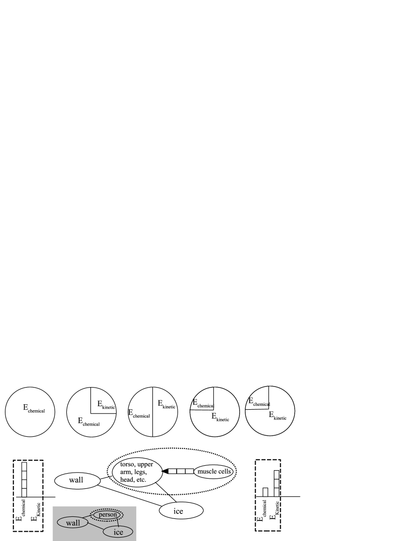
Figure 6: Energy pie charts, bar graphs and flow diagram for a skater on frictionless ice pushing off of a rigid wall. Once again, the inset shows a simpler energy flow diagram in which the person is treated as a single object. Both versions are correct. Which option you choose depends on the level of detail appropriate for your students and on the concepts you wish to emphasize.

If students first gain sufficient practice using the diagrams and graphs to express and refine their ideas, starting with easier problems and progressing in difficulty, they will continue to use them - and by implication the conceptual analysis they represent - as the starting point for quantitative analysis. To help students move from a conceptual-visual analysis to equations, the curriculum must now provide expressions for amounts of energy stored and transferred, as well as a way to associate those expressions with different parts of the diagrams and graphs, and by implication with the concepts those parts represent. The overall structure of the diagrams and graphs then allows the student to write an appropriate conservation of energy equation. In section III, I will use a two-particle model to derive appropriate expressions for internal energy and associate them with the visual representations. In section IV, I simplify those results to four physically sensible guidelines and show how they can be used to solve the problems we have just examined conceptually. This theory is mathematically equivalent to previous theories of internal energy in introductory physics, but my approach is designed to fit much better with the conceptual and visual introduction.

III The two-particle model

To apply energy to complex systems, it can be assumed that a macroscopic object is composed of structureless point particles interacting with each other by means of conservative, central forces. I will closely follow the development of multi-body theory in David Hestenes’ New Foundations for Mechanics,Hestenes-NFCM but will apply it only to a two-particle system. The mathematical development is guided by the idea that the term “work” should receive a clear conceptual definition as energy that is transferred through the boundary of a system; a mathematical expression will be identified as work - of any sort - only when it corresponds to this definition. The two-particle results can be generalized to a system with an arbitrarily large, but finite number of particles and the conclusions are similar.

Our system will be composed of two particles with masses $m_{1}$ and $m_{2}$, positions $\mathbf{X}_{1}$and $\mathbf{X}_{2}$ and exerting mutual forces $\mathbf{f}_{12}$ and $\mathbf{f}_{21}$, assumed to obey the third law, to be conservative, directed along the line joining the two particles, and to depend only on their relative position, $\mathbf{r}=$$\mathbf{X\mathrm{{}_{1}-\mathbf{X\mathrm{{}_{2}}}}}$. External objects exert a total force $\mathbf{F}_{1}$ on particle 1 and total force $\mathbf{F}_{2}$ on particle 2. In other words:

$$\mathbf{f}_{12}=-\mathbf{f}_{21}=\frac{f_{12}\left(\mathbf{r}\right)\mathbf{r}}{r} and \int_{\mathbf{r}_{o}}^{\mathbf{r}_{f}}\mathbf{f}_{12}\cdot d\mathbf{r}=-\Delta U_{int}$$ (1)

$$m_{1}\mathbf{A\mathrm{{}_{1}=\mathbf{F\mathrm{{}_{1}+\mathbf{f\mathrm{{}_{12}}}}}}} m_{2}\mathbf{A\mathrm{{}_{2}}=}\mathbf{F\mathrm{{}_{2}+\mathbf{f\mathrm{{}_{21}=\mathbf{F\mathrm{{}_{2}-\mathbf{f\mathrm{{}_{12}}}}}}}}}$$ (2)

Since these assumptions are properties of almost all fundamental interactions between elementary particles, the multi-body theory we develop will have broad applicability.

Hestenes begins his analysis with the following observation:

To analyze the behavior of a system, we must separate it from its environment. This is done by distinguishing external and internal variables. The external variables describe the system as a whole and its interaction with other (external) systems. The internal variables describe the (internal) structure of the system and the interactions among its parts.

For the system of both particles, the external variables include:

$$\mathrm{total\>mass} M=m_{1}+m_{2}$$ (3)

$$\mathrm{total\>external\>force} \mathbf{F}=\mathbf{F}_{1}+\mathbf{F}_{2}$$ (4)

$$\mathrm{center\>of\>mass} \mathbf{X}=\frac{m_{1}\mathbf{X}_{1}+m_{2}\mathbf{X}_{2}}{M}$$ (5)

$$\mathrm{velocity\>of\>center\>of\>mass} \mathbf{V}=\frac{d\mathbf{X}}{dt}=\frac{m_{1}\mathbf{V}_{1}+m_{2}\mathbf{V}_{2}}{M}$$ (6)

$$\mathrm{acceleration\>of\>center\>of\>mass} \mathbf{A}=\frac{d\mathbf{V}}{dt}=\frac{m_{1}\mathbf{A}_{1}+m_{2}\mathbf{A}_{2}}{M}$$ (7)

$$\mathrm{translational\>(or\>center\>of\>mass)\>kinetic\>energy} E_{kinetic-cm}=\frac{1}{2}MV^{2}$$ (8)

The internal variables describe the motion of the particles relative to the center of mass as well as their interactions with each other. These include $m_{1}$, $m_{2}$, $\mathbf{f}_{12}=-\mathbf{f}_{21}$ and $\bigtriangleup U_{int}$ as well as:

$$\mathbf{v}_{1}=\mathbf{V}_{1}-\mathbf{V} \mathbf{v}_{2}=\mathbf{V}_{2}-\mathbf{V}$$ (9)

$$Internal\>Kinetic\>Energy E_{kinetic-int}=\frac{1}{2}m_{1}v_{1}^{2}+\frac{1}{2}m_{2}v_{2}^{2}$$ (10)

$$Total\>Internal\>Energy \bigtriangleup E_{int}=\bigtriangleup E_{kinetic-int}+\bigtriangleup U_{int}$$ (11)

Notice that I use capital letters with subscripts to refer to individual particle variables, plain capital letters to refer to external variables, and lower-case letters to refer to internal variables.

The total internal energy of a multi-particle system is the sum of the kinetic energy due to motion of the particles relative to the center of mass and the potential energy stored in the fields between the particles, which depends on the inter-particle distances. While it is straightforward to account for the internal energy of a two-particle system by simply adding these terms, the method quickly becomes unwieldy as the number of particles in the system increases. For large systems, it is usually easier to reorganize equation 11 into a smaller number of terms that are more accessible to macroscopic measurements. Hence, the internal energy includes the thermal energy due to oscillations of the particles in the system. When the system changes shape because it is compressed, stretched or bent in any way, then inter-particle distances must change, altering the internal potential energy. If such deformations are elastic, then internal kinetic energy may later change as some part of the system recovers by “springing back.” If the system is capable of undergoing a change in phase or a chemical change, the resulting changes in inter-particle distances and configurations will change the internal energy as well.thermo-mech Although it may not be immediately obvious, the internal energy also includes rotational kinetic energy. Consider the case of a rigid body, for which the distances of each particle relative to the center of mass as well as relative to each other are fixed. In that case, the only way particles can move relative to the center of mass is if the entire object rotates with angular velocity $\boldsymbol{\omega}$, so that $E_{kinetic-int}=\frac{1}{2}m_{1}v_{1}^{2}+\frac{1}{2}m_{2}v_{2}^{2}=\frac{1}{2}m_{1}r_{1}^{2}\left(\frac{v_{1}}{r_{1}}\right)^{2}+\frac{1}{2}m_{2}r_{2}^{2}\left(\frac{v_{2}}{r_{2}}\right)^{2}=\frac{1}{2}\left(m_{1}r_{1}^{2}+m_{2}r_{2}^{2}\right)\omega^{2}=\frac{1}{2}I\omega^{2}$, where $r_{i}=\frac{\left|\mathbf{\boldsymbol{\omega}\times}\mathbf{r}_{i}\right|}{\omega}$ is the distance of the ith particle from the axis of rotation and I is the moment of inertia about that axis. Introductory texts usually include a lengthier derivation of rotational kinetic energy and moment of inertia, and it could be said that I am now applying a similar treatment to all internal energy.

The total kinetic energy is the sum of the kinetic energy of the two particles, but it can be separated into internal and external parts using equations 9 , 6 and 3.KE-total-multi

$$E_{kinetic-total}=\frac{1}{2}m_{1}V_{1}^{2}+\frac{1}{2}m_{2}V_{2}^{2}=\frac{1}{2}m_{1}\left(\mathbf{v}_{1}+\mathbf{V}\right)\cdot\left(\mathbf{v}_{1}+\mathbf{V}\right)+\frac{1}{2}m_{2}\left(\mathbf{v}_{2}+\mathbf{V}\right)\cdot\left(\mathbf{v}_{2}+\mathbf{V}\right)\\ =\frac{1}{2}\left(m_{1}+m_{2}\right)V^{2}+\frac{1}{2}m_{1}v_{1}^{2}+\frac{1}{2}m_{2}v_{2}^{2}+\mathbf{V}\cdot\left(m_{1}\mathbf{v}_{1}+m_{2}\mathbf{v}_{2}\right)=E_{kinetic-cm}+E_{kinetic-int}$$ (12)

To relate changes in kinetic energy to the forces on the system, we take the derivative of 12 and use 2.

$$\frac{dE_{kinetic-total}}{dt} = \frac{d}{dt}\left(\frac{1}{2}m_{1}\mathbf{V}_{1}\cdot\mathbf{V}_{1}+\frac{1}{2}m_{2}\mathbf{V}_{2}\cdot\mathbf{V}_{2}\right)=m_{1}\mathbf{V}_{1}\cdot\frac{d\mathbf{V}_{1}}{dt}+m_{2}\mathbf{V}_{2}\cdot\frac{d\mathbf{V}_{2}}{dt}$$ (13)

$$= \mathbf{V}_{1}\cdot\left(m_{1}\mathbf{A}_{1}\right)+\mathbf{V}_{2}\cdot\left(m_{2}\mathbf{A}_{2}\right)=\left(\mathbf{F}_{1}+\mathbf{f}_{12}\right)\cdot\mathbf{V}_{1}+\left(\mathbf{F}_{2}+\mathbf{f}_{21}\right)\cdot\mathbf{V}_{2}$$

$$\frac{dE_{kinetic-total}}{dt} = \frac{dE_{kinetic-cm}}{dt}+\frac{dE_{kinetic-int}}{dt}=\left(\mathbf{F}_{1}\cdot\mathbf{V}_{1}+\mathbf{F}_{2}\cdot\mathbf{V}_{2}\right)+\left(\mathbf{f}_{12}\cdot\mathbf{V}_{1}+\mathbf{f}_{21}\cdot\mathbf{V}_{2}\right).$$

The right-hand side of equation 13 can be expressed in terms of internal and external variables using equations 9 and 4 .int-ext-power-multi

$$\mathbf{F}_{1}\cdot\mathbf{V}_{1}+\mathbf{F}_{2}\cdot\mathbf{V}_{2} \mathbf{=F}_{1}\cdot\left(\mathbf{v}_{1}+\mathbf{V}\right)+\mathbf{F}_{2}\cdot\left(\mathbf{v}_{2}+\mathbf{V}\right) =\mathbf{F}\cdot\mathbf{V}+\left(\mathbf{F}_{1}\cdot\mathbf{v}_{1}+\mathbf{F}_{2}\cdot\mathbf{v}_{2}\right)$$ (14)

$$\mathbf{f}_{12}\cdot\mathbf{V}_{1}+\mathbf{f}_{21}\cdot\mathbf{V}_{2} =\mathbf{f}_{12}\cdot\left(\mathbf{v}_{1}+\mathbf{V}\right)-\mathbf{f}_{12}\cdot\left(\mathbf{v}_{2}+\mathbf{V}\right) =\mathbf{f}_{12}\cdot\left(\mathbf{v}_{1}-\mathbf{v}_{2}\right)=\mathbf{f}_{12}\cdot\mathbf{v},$$ (15)

where the relative velocity is $\mathbf{v}=\mathbf{V}_{1}-\mathbf{V}_{2}=\mathbf{v}_{1}-\mathbf{v}_{2}=\frac{d\mathbf{r}}{dt}$. Combining equation 13 with equations 14 and 15 then anti-differentiating and using 1 and 11, we find:

$$\bigtriangleup E_{kinetic-cm}+\bigtriangleup E_{int}=\bigtriangleup E_{kinetic-cm}+\bigtriangleup E_{kinetic-int}+\bigtriangleup U_{int}=\int_{\mathbf{X}_{0}}^{\mathbf{X}_{f}}\mathbf{F}\cdot d\mathbf{X}+\int_{\mathbf{X}_{10}}^{\mathbf{X}_{1f}}\mathbf{F}_{1}\cdot d\mathbf{x}_{1}+\int_{\mathbf{X}_{20}}^{\mathbf{X}_{2f}}\mathbf{F}_{2}\cdot d\mathbf{x}_{2}$$ (16)

This is the full energy equation for our two-particle system. It presents us with a sum of three integrals involving dot-products of force and displacement. In keeping with the previously mentioned guideline, I defer defining any of these integrals as work until it can be determined whether they represent energy transferred through the boundary of the two-particle system. The last two integrals become easier to interpret if the purely external terms are subtracted from the equation. Start by differentiating equation 8 and using 2, 4 and 7 to obtain $\frac{dE_{kinetic-cm}}{dt}=M\mathbf{V}\cdot\frac{d\mathbf{V}}{dt}=\mathbf{V}\cdot\left(M\mathbf{A}\right)=\mathbf{F}\cdot\mathbf{V}$, which can be anti-differentiated to obtain:

$$\bigtriangleup E_{kinetic-cm}=\int_{\mathbf{X}_{0}}^{\mathbf{X}_{f}}\mathbf{F}\cdot d\mathbf{X}$$ (17)

Subtracting equation 17 from equation 16, we find the remaining terms are related by:

$$\bigtriangleup E_{int}=\int_{\mathbf{X}_{10}}^{\mathbf{X}_{1f}}\mathbf{F}_{1}\cdot d\mathbf{x}_{1}+\int_{\mathbf{X}_{20}}^{\mathbf{X}_{2f}}\mathbf{F}_{2}\cdot d\mathbf{x}_{2}$$ (18)

To paraphrase HestenesHestenes-NFCM , this equation describes alteration of the internal energy by external forces. Specifically this occurs when external objects force particles of the system to move relative to the center of mass. This implies rotation and/or deformation of the system, both visible consequences of external forces that can alert students to internal energy transfers as they gradually build a complete concept of energy. It is precisely when the system is rotated or deformed that it cannot be approximated as a single particle and a two-particle model becomes the simplest approach that retains an accurate understanding of energy.

This not only provides a meaning for the last two integrals in equation 16, it tells us that the integral in equation 17 can be interpreted as the work only when the the external forces cause no changes in internal energy so that the two integrals in equation 18 sum to zero. In that case, the only source for the change in center of mass kinetic energy is the external object or objects exerting the force $\mathbf{F}$. Of course, one case where this obtains is a single-particle system, which is the starting point for energy analysis in most introductory texts. While equation 17 says literally that the integral of the dot product of force and center of mass displacement equals a change in center of mass (translational) kinetic energy, many texts proceed to adopt $\int_{\mathbf{X}_{0}}^{\mathbf{X}_{f}}\mathbf{F}\cdot d\mathbf{X}$as a general definition of work and apply this definition outside its limited range of validity. As section II shows, situations where external forces cause changes in internal energy are quite common and are almost always included among the examples and problems in these same introductory texts. Conceptual confusion sets in when $\int_{\mathbf{X}_{0}}^{\mathbf{X}_{f}}\mathbf{F}\cdot d\mathbf{X}$ is called “work” but does not represent energy transfer through the system boundary. It is not equation 17 itself which is the problem, but its interpretation as a general definition of work which leads to conceptual difficulties. Other authors arons ; arons-book ; Mungan-review ; sherwood-pseudowork ; swackhamer-work-work ; mall-leff-all-about-work recognize the limits of the definition and supplement equation 17 with a multi-particle energy equation while inventing names such as “particle work” or “pseudo work” to identify$\int_{\mathbf{X}_{0}}^{\mathbf{X}_{f}}\mathbf{F}\cdot d\mathbf{X}$ in troublesome situations. As an alternative, I continue the mathematical development without applying names until I can clearly identify which integrals truly represent energy transferred through the system boundary.

Our investigation of two-particle models has produced two different types of force vs. distance integrals, which differ in the choice of external or internal variables for the position. For example, $\int_{\mathbf{X}_{10}}^{\mathbf{X}_{1f}}\mathbf{F}_{1}\cdot d\mathbf{x}_{1}$ can be used to calculate an amount of energy transferred from external objects to particle 1 and stored internally by the system. On the other hand, $\int_{\mathbf{X}_{10}}^{\mathbf{X}_{1f}}\mathbf{F}_{1}\cdot d\mathbf{X}$ (which is part of $\int_{\mathbf{X}_{0}}^{\mathbf{X}_{f}}\mathbf{F}\cdot d\mathbf{X}$ because of equation 4) represents energy transferred from external objects to particle 1 and stored as translational kinetic energy of the system. In addition, these two integrals can be added to get:

$$\int_{\mathbf{X}_{10}}^{\mathbf{X}_{1f}}\mathbf{F}_{1}\cdot d\mathbf{x}_{1}+\int_{\mathbf{X}_{10}}^{\mathbf{X}_{1f}}\mathbf{F}_{1}\cdot d\mathbf{X}=\int_{\mathbf{X}_{10}}^{\mathbf{X}_{1f}}\mathbf{F}_{1}\cdot d\left(\mathbf{x}_{1}+\mathbf{X}\right)=\int_{\mathbf{X}_{10}}^{\mathbf{X}_{1f}}\mathbf{F}_{1}\cdot d\mathbf{X}_{1}$$ (19)

The right-hand side of this equation involves the total force from external objects on particle 1 as well as the total displacement of particle 1. This is the total amount of energy transferred from external objects to particle 1, and thus to the system. To be consistent with the thermodynamic definition of work as the energy transferred through the system boundary, this must be the work done by forces $\mathbf{F}_{1}$ on the system. The left side of equation 19 (along with equations 17 and 16) tells us that this total energy transfer accounts for a portion of the changes in internal energy and translational kinetic energy. While this may seem abstract, when solving elementary problems it is often possible to model the system as two particles, one particle located at the point of application of the force and another located at the center of mass and representing the rest of the object. From there, one can identify displacement of the center of mass, displacement of the first particle relative to the center of mass and total displacement of the particle. Even when one or more of these displacements is unknowable, distinguishing among the three cases can aid an analysis of energy storage and transfer and help resolve confusion.

The interpretation of force vs. displacement integrals in this paper, in particular the decision to apply the term work in general to equation 19 but not equations 17 or 18, is a direct consequence of adopting an appropriate mathematical model - one capable of representing internal energy because the system includes more than one particle - and strictly defining “work” in accord with thermodynamics, as the amount of energy transferred from external objects through the boundary of the system. Mallinckrodt and Leffmall-leff-all-about-work define seven different force vs. displacement integrals that appear in the literature, but point out that only three of these are independent. Starting with any three, the other four may be determined by simple mathematical relationships. My choice of three integrals is therefore a sufficient set and mathematically equivalent to prior formulations. Mallinckrodt and Leff generally regard this choice as the easiest set of three to understand and apply.

Finally, it should be noted that when external objects exert conservative forces on the multi-particle system, the system may be enlarged to include these objects and introduce external potential energy terms to the left-hand side of equation 16. However, changes to the internal energy may also occur if the forces in question are not uniform. Tidal forces are one example of this, and they work precisely because non-uniform gravitational forces deform an object by displacing parts of it relative to the center of mass. Use of two-particle models for elementary problems can help prepare students for the study of more advanced topics, such as tidal forces, when they encounter them later in their studies. In many cases, the external conservative force is approximately uniform and will therefore cause only negligible changes in internal energy.

IV Solving problems by combining diagrams, graphs and mathematics

Zou and vanHeuvelen outline a general problem-solving procedure when employing diagrams and graphs.vanHeuvelen-zou The student first analyzes energy storage and transfer using the pie charts, bar graphs, and energy flow diagrams as in section II. In the case of a deformable or rotating system, the guidelines developed in section III help the student associate each energy formula with the appropriate energy transfer or storage mechanism. There are three displacements to examine for each external force: the displacement $\mathbf{X}$ of the center of mass, the displacement $\mathbf{x}$ - relative to the center of mass - of the particle to which the force is directly applied, and the total displacement $\mathbf{X}_{1}=\mathbf{x}+\mathbf{X}$ of that particle. If the force is constant, $FX\cos\theta$ will equal the change in translational kinetic energy; $Fx\cos\theta$ equals the change in internal energy; and $FX_{1}\cos\theta$ equals the total energy transferred from the external object to the system, which is the work. For basic mechanics, the kinetic energy formula is also necessary. Others, such as the specific heat formula, can be added as the course sequence dictates. The student associates each energy formula with one or more parts of the diagrams, and reads a conservation of energy equation from the overall structure. The only necessary mathematical change to the curriculum is to provide students with the meaning of the above three products in lieu of defining work as $FX\cos\theta$. The mathematical manipulations achieved by this procedure are identical to those recommended by previous authors. The single particle energy model is discarded, and students learn a multi-particle theory first conceptually and then mathematically. When appropriate, the conservation of energy equation obtained by this procedure will automatically simplify to the single-particle work-energy equation.

Figure 7: Internal, external and total particle displacements for the two-puck-and-string problem.

Figure 7 is a more complete diagram for the two-pucks-and-string problem from section II, which reveals that the point of application of the force (the center of the string) has been displaced relative to the center of mass, causing the system to change shape. Hence, we know that $FX$ will not equal the work. Instead, figure 8 shows how to correctly associate energy formulas with parts of the diagrams. $FX=\frac{1}{2}\left(2m\right)V^{2}$, because products with the center of mass displacement equal changes in translational kinetic energy. $Fx=F\left(X_{1}-X\right)=2mC\Delta T$ (where C is the specific heat and T is the temperature) because products with the internal displacement equal the changes in internal energy, which is thermal in this case. Finally, $FX_{1}=\frac{1}{2}\left(2m\right)V^{2}+2mC\Delta T$, because the total work done by the person is transferred to the pucks and stored both internally and externally. There is a clear conceptual interpretation for each product of force and displacement, and it is clear that $FX_{1}$ is the work, while $FX$ and $Fx$ are not.2pucks-confirm A student who can draw correct diagrams, explain the meaning of those diagrams in words, and associate each part of their calculation with part of a diagram has demonstrated a thorough understanding both conceptually and mathematically. The mathematics is not only consistent with the conceptual analysis, it follows directly from the concepts in a straightforward manner. A larger portion of the energy unit may be spent on conceptual analysis, because the structure of the diagrams and graphs leads so neatly into the conservation of energy equation. Students are far less likely to make common mathematical mistakes such as negative sign errors or double accounting for work and potential energy, so less time is required to address mathematical difficulties.

Figure 8: Mathematical expressions and equations have been added to the energy bar graphs and flow diagram from figure 3 to show how each corresponds to one or more parts of the diagram. The structure of the diagrams and graphs leads directly to a conservation of energy equation.

The frictional force on a car, or any object, skidding to a stop is actually the sum of many microscopic forces between the surface (the road) and the skidding object (the car).sherwood-heat-work As the car skids forward, a “tooth” from the uneven road surface exerts an external force $\mathbf{f}$ on a tooth of the car tire opposite to the direction of travel (see figure 9). This causes a negative change in the center of mass kinetic energy equal to $-fX$, because the frictional force is opposite the displacement of the center of mass, $\mathbf{X}$. It causes a positive change in the internal energy equal to $fx$, because the frictional force and the internal displacement of the tire atom, $x$ are in the same direction, both opposite the motion. And there is a net transfer of energy out of the system equal to $-f\left(X-x\right)=-fX_{1}$. $-fX_{1}$ is the work, but we are unable to calculate an exact value without knowing the microscopic displacement $x$. The total energy transfer will be the sum of similar terms over all of the atoms of the tire in contact with atoms of the road. While we cannot calculate the work, if the total external frictional force and the displacement of the center of mass are known, we can calculate the total change in the translational kinetic energy of the center of mass. This is the calculation typically accepted as a solution to this problem, and it is mathematically correct. However, it is conceptually misleading to claim that it expresses the idea that work done by the frictional force equals the change in the kinetic energy. It does not. negative-signs

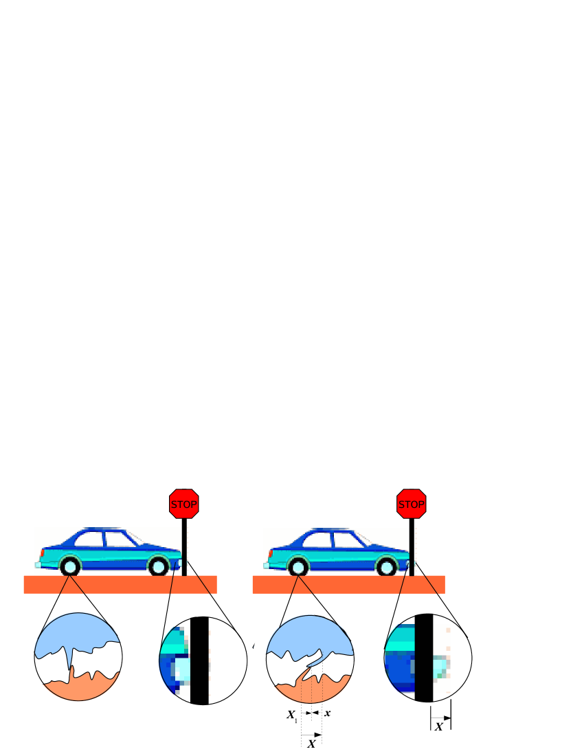
Figure 9: Internal and External Variables for an Object Skidding to a Stop. The car starts to skid at the instant its front end reaches the pole of the stop sign. The second and fourth blowups show the car moving a very small (actually microscopic) distance $\mathbf{X}$ during the first few instants of the skid. The first and third blowups are inspired by Sherwood and Bernard’s “stylized microscopic view of friction, with greatly exaggerated vertical scale,” showing that “teeth” belonging to the tire and the road surface have welded together at their contact point.sherwood-heat-work The upper tooth is carried forward a distance $\mathbf{X}$. The point where the force is applied at the tip of the tooth is displaced a distance $\mathbf{x}$ to the left relative to the center of mass, but relative to the lower tooth, it is displaced a distance $\mathbf{X}_{1}=\mathbf{X}-\mathbf{x}$ to the right. Scales in this figure have been exaggerated disproportionately for the sake of clear presentation of the relation among the displacement vectors.

Figure 10: Internal and external variables for a skater on frictionless ice pushing off of a wall. The person’s center of mass was displaced a distance $\mathbf{X}$ during the push, while the point of application of the force was displaced an equal amount in the opposite direction, relative to the center of mass, but was not displaced at all relative to the wall.

Recall the skater pushing off of the wall? The diagrams in section II showed that no work was done because no energy was transferred from the wall to the person. The person changes shape or is “deformed” when the point of application of the force, the person’s hands, is displaced relative to the center of mass. Therefore, we know that $FX$ will not equal the work. In more detail, figure 10 shows that the person’s center of mass was displaced a distance $\mathbf{X}$ during the push, while the point of application of the force was displaced an equal amount in the opposite direction, relative to the center of mass, but was not displaced at all relative to the wall. $FX$ represents an increase in the translational kinetic energy of the person. $-Fx$ represents an equal decrease in the internal energy of the person, corresponding exactly with our conceptual analysis. Finally $FX_{1}$ is the work, the amount of energy transferred from the wall to the person, and it is indeed zero.

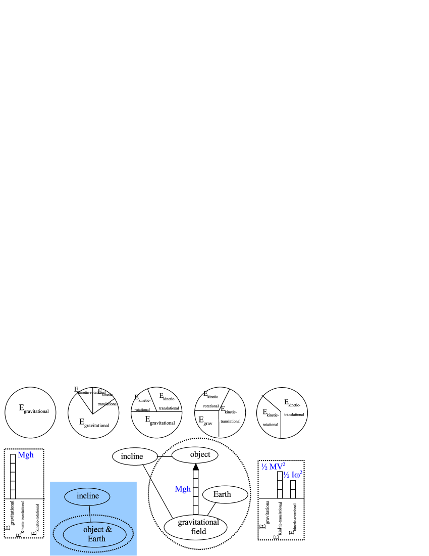
Figure 11: Energy pie charts, bar graphs and flow diagram for a round object rolling down an incline. The inset shows a simpler energy flow diagram in which the round object, the Earth and by implication also the gravitational field are treated as a single object. Both versions are correct. Which option you choose depends on the level of detail appropriate for your students, in particular their readiness to deal with the concept of the field as real physical object which, although invisible, stores the gravitational potential energy.sherwood-gravity

Figure 12: Infinitesimal Internal and External Displacements for a Rolling Object - In an infinitesimal time interval $\Delta t$, the center of mass of a rolling object is displaced by an amount $\mathbf{X}$, and the original point of contact is displaced by an amount $\mathbf{\mathbf{x}}$ relative to the center of mass. If the object rolls without slipping, $\mathbf{\mathbf{x}}$ is approximately equal in magnitude but opposite in direction to $\mathbf{X}$, so that in the limit that $\Delta t$ approaches zero, the displacement of the point of contact is also zero.

As a final example, consider a round object of mass M, radius R and moment of inertia $I=bMR^{2}$, where b is a unitless fraction equal to $\frac{2}{5}$ for a sphere or $\frac{1}{2}$ for a cylinder, etc. When the object starts from rest and rolls without slipping down an incline of height $H$ and length $L$, gravitational energy is transferred to translational kinetic energy plus rotational kinetic energy, as shown in figure 11. This gives $MgH=\frac{1}{2}MV^{2}+\frac{1}{2}I\omega^{2}=\frac{1}{2}MV^{2}\left(1+b\right),$where $V=\omega R$ because the object does not slip. The static frictional force, $f$ acts opposite the direction of motion while the object’s center of mass is displaced a distance $L$ down the incline. The meaning of the product $fL$ can be determined by examining infinitesimal displacements of a rolling object, as shown in figure 12. Because the point of application of the frictional force (where the object contacts the ground) is displaced relative to the center of mass, we can anticipate that the dot product of the frictional force and the displacement of the center of mass will not equal the work. The frictional force $f$ is opposite in direction to the displacement of the center of mass $X$, leading to a decrease in the object’s translational kinetic energy, $-fX=\Delta\left(\frac{1}{2}MV^{2}\right)$. On the other hand, $f$ is in approximately the same direction as the internal displacement, $x$, leading to an increase in the object’s internal energy, $fx=\Delta\left(\frac{1}{2}I\omega^{2}\right)$. If the object rolls without slipping, then in the limit $\Delta t$ approaches zero, $\mathbf{x}$ is equal and opposite to $\mathbf{X}$, so that the instantaneous displacement of the point of contact is $\mathbf{X\mathrm{{}_{1}}=}\mathbf{X-x\mathrm{=0}}$ and no work is done. The action of the frictional force is to transfer energy from translational kinetic energy to rotational kinetic energy without doing any work because the energy remains in the system at all times.w-e-roll Hence, there is no energy flow arrow betwen the incline and the object in figure 11, and we can conclude that $fL=\Delta KE_{rotational}=\frac{bMgH}{b+1}=\frac{1}{2}I\omega^{2}$. Carnero et. al, Sherwood and Mungan obtain the same result,carnero-roll-work ; Mungan-review ; sherwood-pseudowork but the meaning of the force-displacement products derived from the two particle model provides a much more straightforward path to this solution. Although one cannot strictly model a rolling object with a two-particle model, the introduction of two-particle models earlier in the course sequence prepares students for a more sophisticated understanding of work and energy in rolling motion, as a comparison of the pairs of equal and opposite displacements in figures 10 and 12 shows.

V conclusion

One goal of a good introductory physics course should be for students to develop a useful model of energy and its conservation, one that they can employ to understand energy concepts throughout their lives. Teachers must take care to present the material in a logical sequence so that concepts are continually refined and ideas build on one another. At the introductory level, the mathematics should be kept as simple as possible, but a certain level of complexity is necessary in order to support the development of correct energy concepts. In this conclusion, I will outline some successful reforms of the pedagogical sequence for teaching energy, point out where two-particle models fit into this sequence, and show how the inclusion of two-particle models for some elementary problems can help prepare students for more advanced topics.

The overarching theme of Eric Brewe’s doctoral disserationbrewe is “energy early, energy often, energy intuition.” He spends approximately the same amount of class time on energy as he would in a more standard course sequence, but instead of covering energy all at once, he weaves in an energy thread throughout. During the first week, he teaches students to represent their energy ideas qualitatively using pie charts and system schemas.system-schema At some point during each unit, he revisits energy by applying these representational tools to new situations, while gradually refining the existing tools and adding others - energy flow arrows on system schemas, bar graphs, equations and potential graphs. Students do not use energy equations until they have developed a more sophisticated understanding of energy conservation. It is important that students practice using the diagrams and graphs to express energy ideas for some time before proceeding to equations. If they are comfortable with the representational tools, they will continue to use them as an aid to problem-solving. The result of Brewe’s reform is greater comfort with energy as a problem-solving alternative and a greater understanding of its relation to other topics.extension-to-modeling

Within Brewe’s sequence, two-particle models should not be introduced until students understand how to apply the representational tools and equations to simpler situations. These include situations in which internal energy changes are negligible, as well as other cases, such as many inelastic or partially elastic collisions, where modeling objects as single particles that can store internal energy may be sufficient. In the two puck and string problem, for instance, we did just that when we assumed that a portion of the pucks’ kinetic energy was transferred to thermal energy when they collided. Once students have an appropriate background, examples such as those from section II can be used to help them refine their definition of work and to develop a deeper understanding of energy storage and transfer. Because the conceptual development has included internal energy from the start and the structure of the diagrams leads directly to the equations, one need only introduce the meaning of the three different force vs. displacement products to apply the two-particle model.

A common bouncing ball occupies a pivotal point in the calculus-based college physics course as taught by Dwayne Desbian, and shows how students can be led to understand the difference between a single-particle and a multi-particle model.desbain This situation contains basic elements of almost all of the examples in this paper. The floor causes the ball to flex as it comes momentarily to rest, in a manner similar to the way the brick wall crumples the car’s front end. As the ball rebounds, some of the energy is restored to kinetic energy because of the elastic flexing of the ball’s material. This energy does not come from the floor, but in a manner similar to the jumping person or the skater pushing off from the wall, it remains stored in the ball the entire time. Even though the ball may store less kinetic energy after the bounce than before, that does not mean the energy has left the ball. Similar to the car skidding to a stop, the energy is at least partially stored as thermal energy in the ball itself. Through careful consideration of this problem using all of the different representations, students in Desbian’s course discover the failure of the single particle model and develop a model of the ball as two particles mediated by a linear restoring force.

I showed in section IV how an early introduction to internal energy better prepares students to understand energy transfer when objects roll without slipping. Students who continue their physics education will be exposed to ideas of internal energy and deformation in even more complicated contexts, including thermodynamics, molecular dynamics, solid-state physics, and atomic physics.alonso-finn2 In thermodynamics, students encounter difficulty understanding the work done on or by the working fluid of a heat engine. Problems such as the skater and the car crash provide more concrete and familiar contexts in which to associate compression and expansion of the system with changes in internal energy. The two-particle, linear-restoring-force model of the bouncing ball is important in its own right. Although seemingly simple, it contains the basic ideas of elastic behavior, and internal oscillations leading to thermal energy.mungan-2blocks-spring In their introductory physics course, Matter and Interactions, Ruth Chabay and Bruce Sherwood make innovative use of particles connected by linear restoring forces to demonstrate how bulk properties of matter emerge by applying basic mechanics to its constituent parts.m&i This is the central concept of solid state physics. In atomic physics, absorption or emission of a photon leads to changes in the internal energy of an atom, accompanied by deformation in the form of changes in its size and shape. Once students express atomic transitions using the familiar bar graphs and energy flow diagrams, they find energy level diagrams much easier to comprehend. Tides and other phenomena due to the action of non-uniform fields can be understood through internal energy transfers accompanied by deformation. Introducing two-particle models at the introductory level also exposes students to the idea of a model and its limits, and helps them to understand multi-body theory when they encounter it in an advanced physics course.

Teaching energy using multiple representations to promote student-to-student dialog is gaining currency among physics teachers. This paper is but the latest in a long series of efforts to deal with the mathematics of internal energy at the introductory level. Both mathematical and visual approaches are finding their way into current textbooks. On the other hand, a unitary fluid-like metaphor for energy, a more rigorous expression of conservation of energy, an elevation of the importance of diagrams and graphs relative to equations, or the idea that $\int\mathbf{F}\cdot d\mathbf{X}$ does not, in general, equal work are counter-intuitive ideas to many trained physicists and introductory physics teachers. When they encounter these ideas in the PER literature, it may well cause them to disregard the reform efforts. It is my hope that combining the mathematical and visual approaches and clarifying the mathematical and theoretical basis for these reforms will help some physicists and teachers take a closer look at the real value of the proposed changes.

Matt Greenwolfe

grew up in Indiana and received a B.S. degree in physics from Washington University in St. Louis and a PhD in physics from The University of Michigan. Over the past eleven years his high school classes have evolved to use guided inquiry, student discourse, and multiple representations. He is currently president of the American Modeling Teachers Association, www.modelingteachers.org.

- (1) Bruce Sherwood, “Pseudowork and real work,” Am. J. Phys. 51, 597 (July 1983).
- (2) A.B. Arons, “Development of energy concepts in introductory physics courses,” Am. J. Phys. 67, 1063-1067 (Dec. 1999).
- (3) M. Alonso and E.J. Finn, “On the notion of internal energy,” Phys. Educ. 32, 256-264 (July 1997).
- (4) Carl E. Mungan, “A primer on work energy relationships for introductory physics,” The Physics Teacher 43, 10 - 16 (January 2005).
- (5) A. John Mallinckrodt and Harvey F. Leff, “All about work,” Am. J. Phys. 60, 1063-1067 (April 1992).
- (6) Although the use of the work-energy theorem is also usually accompanied with a warning to the effect that it does not give valid information about work and energy, but is merely a useful dynamical relationship among the variables.
- (7) See for example, Clifford Swartz, “Why use the work-energy theorem?” Am. J. Phys. 72 (Sept. 2004).
- (8) Alan Van Heuvelen and Xueli Zou, “Multiple representations of work and energy processes,” Am. J. Phys. 69, 184 - 194 (Feb. 2001).
- (9) G. Falk and F. Herrmann, eds., KonzepteeineszeitgemssenPhysikunterrichts, 5 vols., (Schroedel Verlag, Hannover, 1982).
- (10) Gregg Swackhamer, “Making work work,” http://modeling.asu.edu/modeling/MakingWorkWork.pdf (Feb. 2005).
- (11) Malcolm Wells, David Hestenes, Gregg Swackhamer, Larry Dukerich and collaborators, “Modeling Materials in Mechanics, Unit 0: An Integrated Approach to Energy,” http://modeling.asu.edu/Modeling-pub/Mechanics_curriculum/0-Energy-Preface/0_U0%20TeacherNotes.pdf (2002).
- (12) Implied with these definitions is a unitary metaphor for energy as a conserved fluid-like substance. While physical objects change when they gain or lose energy, the energy itself does not change type or form, but is merely transferred from place to place and stored in different ways. See G. Falk, F. Herrmann, and G.B. Schmid, “Energy forms or energy carriers?” Am. J. Phys. 51, 1074-1077 (Dec. 1983).
- (13) K. A. Legge and J. Petrolito, ”The use of models in problems of energy conservation,” Am.J. Phys. 72, 436-438 (April 2004).
- (14) For an example of how to incorporate models and their scope throughout introductory physics, see Eugenia Etkina, Aaron Warren, and Michael Gentile, “The Role of Models in Physics Instruction,” 44, 34 (Jan. 2006), Malcolm Wells, David Hestenes and Gregg Swackhamer, “A modeling method for physics instruction,” Am.J. Phys. 63, 606 - 619 (July 1995), David Hestenes, “Modeling methodology for physics teachers,” Proceedings of the International Conference on Undergraduate PhysicsEducation (College Park, August 1996) and Malcolm Wells, David Hestenes, Gregg Swackhamer, Larry Dukerich and collaborators, “Modeling Materials in Mechanics,” http://modeling.asu.edu/Modeling-pub/Mechanics_curriculum/ (Dec. 2003).
- (15) Arnold B. Arons, Teaching Introductory Physics (John Wiley and Sons, 1997), p. 145 - 160.
- (16) R.C. Hilborn, “Let’s ban work from physics!” Phys. Teach. 38, 447 (Oct. 2000).
- (17) The single-particle work-energy theorem shows that . FX accounts for only the kinetic energy, but not the thermal energy, and therefore does not account for all of the energy transferred from the person to the system. FX is therefore not equal to the work in this situation.
- (18) In vanHeuvelen and Zou’s study at Ohio State, “The … freshmen learning the multiple representation strategy … performed much better than regular and honors calculus-based physics students …, and they did almost as well as physics faculty and graduate students.”
- (19) Bruce Sherwood and W.H. Bernhard, “Work and heat transfer in the presence of sliding friction,” Am. J. Phys. 61, 121 - 127 (Nov. 1984).
- (20) The single-particle work-energy theorem shows that , where f is the kinetic frictional force between the road and the wheels. But -fX does not equal the work, because it does not account for the thermal energy remaining in the car.
- (21) A. John Mallinckrodt and Harvey F. Leff, “Stopping objects with zero net work: Mechanics meets thermodynamics,” Am. J. Phys. 60, 1063?1067 (Feb. 1993).
- (22) The single-particle work-energy theorem shows that , but if no work is done, this formula cannot be described as work equaling the change in kinetic energy.
- (23) As Sherwoodsherwood-pseudowork states, “It is unfortunately very common to speak of the gravitational potential energy of a person or of a falling rock, but such statements really should be avoided since the Earth must be included in the system.” See also references arons ; falk-herrmann ; vanHeuvelen-zou .
- (24) C. Carnero, J. Aguiar, and J. Hierrezuelo, “The work of the frictional force in rolling motion,” Phys. Educ. 28, 225-227 (July 1993).
- (25) I would also argue that since fL is not work, it should also not be labeled “pseudo-work,” “particle-work,” or “center-of-mass-work.” Such semantic distinctions are likely to confuse an introductory student. On the other hand, student understanding is readily apparent from their attempts to draw the diagrams. If a student can trace where the energy starts, where it is transferred, and where it ends up, then they have a sufficient understanding regardless of the terminology.
- (26) van Heuvelen and ZouvanHeuvelen-zou quote Howard Gunter, “Genuine understanding is most likely to emerge … if people possess a number of ways of representing knowledge of a concept or skill and can move readily back and forth among these different ways of knowing.”
- (27) David Hestenes, New Foundations for Classical Mechanics, 2nd ed. (Kluwer Academic Publishers, 1999), p. 334 - 350. The multi-particle equations we are about to derive also appear among the multiplicity of different work energy relationships derived by Malinckrodt and Leffmall-leff-all-about-work for the general case of N particles.
- (28) With a total of N particles, we get: , , and
- (29) See Mallinckrodt and Leffmall-leff-all-about-work for a more extensive discussion of the relationship between the elementary mechanics of a multi-particle system and thermodynamics, including a discussion of the limitations of this connection.
- (30) Notice that With N particles: = = = = .
- (31) With N particles, 14 is straightforward, But 15 is trickier, , where is the relative velocity of particles i and j. In step 5, I re-wrote the second term swapping the indices and . In the sixth step, I switched the order of the sum and used Newton’s Third Law. Notice that in the final sum, each pair of particles is counted only once.
- (32) In the case of more than two particles, there are still only three types of force vs. displacement integral. See footnote int-ext-power-multi as well as references Hestenes-NFCM and mall-leff-all-about-work for details.
- (33) These results can be confirmed by a more complete treatment of the problem with Newton’s Laws and Kinematics.
- (34) I have been careful with my negative signs here, but this largely unnecessary so long as students can identify the direction of energy flow, which is explicitly indicated in their diagrams and graphs. The negative signs merely reinforce what they should already understand conceptually.
- (35) Eric Thomas Brewe, Inclusion of the EnergyThread in the Introductory Physics Curriculum: an Example of Long-term Conceptual and Thematic Coherence (Arizona State University, 2002). Available at: modeling.asu.edu/modeling/EricBrewe_Dissertation.pdf.
- (36) A system schema is similar to the energy flow diagrams I have used in this paper, except it does not yet include energy flow arrows. In the early stages of the introductory physics course, it is used to help students clearly define a system and identify interactions between the system and its environment. See Lou Turner, “System Schemas,” The Physics Teacher 41, 404 - 408 October 2003.
- (37) His approach is an extension of the energy units in the modeling method of physics instruction, whose materials include more details such as lesson plans, worksheets and tests. See reference modeling .
- (38) Dwain Michael Desbien, Modeling discourse Management Compared to Other Classroom Management Styles in University Physics (Arizona State University, 2002). Available at: http://modeling.asu.edu/modeling/ModelingDiscourseMgmt02.pdf
- (39) See Alonso and Finnalonso-finn for a more detailed discussion.
- (40) See also Mungan’s discussion of two blocks connected by a spring.Mungan-review
- (41) R.W. Chabay and B.A. Sherwood, Matter & Interactions I: Modern Mechanics (Wiley, New York, 2002), Chap. 7.