Super-relativity in the quantum theory

Abstract

The relativity to the measuring device in quantum theory, i.e. the covariance of local dynamical variables relative transformations to moving quantum reference frame in Hilbert space, may be achieved only by the rejection of super-selection rule. In order to avoid the subjective nuance, I emphasis that the notion of “measurement” here, is nothing but the covariant differentiation procedure in the functional quantum phase space $CP(N-1)$, having pure objective sense of evolution. Transition to the local moving quantum reference frame leads to some particle-like solutions of quasi-linear field PDE in the dynamical space-time. Thereby, the functionally covariant quantum dynamics gives the perspective to unify the Einstein relativity and quantum principles which are obviously contradictable under the standard approaches.

PACS 03.65.Ca; 03.65.Ta; 04.20.Cv

1 Introduction

There is some analogy between classical accelerated reference frame in general relativity and moving quantum reference frame in Hilbert space. From the formal point of view in both cases arise physical fields of quite different nature. It would be interesting to find a geometric way to their unification.

The backreaction of the “light” sub-system on the “heavy” sub-system dynamics through a gauge vector and scalar potentials was already geometrized [1]. It comes from the adiabatic Born-Oppenheimer ansatz applied to the coupled sub-systems. On the other hand Aharonov et al made accent on the quantum reference frame - “second particle” reaction described by the effective topological vector potential due to the measurement process [2, 3]. Authors emphasize the necessity of “second particle” usage. Cartan’s method of the moving frame, however, rids us from this obligation. Namely, the quantum state and dynamical variables of a quantum system may be referred to the infinitesimally close previous state. Thereby one is able to restore the objective interpretation of the quantum description. But transition to moving frame in Hilbert space requires the especial control of the elements proximity since the non-adiabatic approximation (where transitions are available) realized by transition to moving frame leads to divergences of the iteration process even for two-level system [4].

The fundamental gauge field coming “from nowhere” in the models of elementary particles, and both Abelian [1] and non-Abelian [5] pseudo-potentials associated with adiabatic Born-Oppenheimer approximation, have formally geometric origin. Pseudo-potentials have a singular source of monopole-like type whose nature arose under degeneration, etc. Dirac put the monopole as a physical source of electromagnetic field. He assumed that singularities are concentrated on some “line of the knots” in the physical space. But the mathematical artefact, say, singularity of mapping cannon be a reason for physical phenomenon. On the other hand monopoles do not exist as physical object up to now; one should have physical mechanism of the fields generation.

The first question is: is it possible to find a non-singular fundamental gauge potential if one uses local coordinates in inherently related projective Hilbert space $CP(N-1)$ instead of the parameter space?

The second question was posed by Berry: “What is the dynamical significance of the moving frame that produce the best approximation to $\gamma$,…?” [1].

There are two reasons of “defeats” of the renormalization procedure by the successive transitions to moving frame [4, 1]. The first of them is lurked in the local (state-dependent) character of embedding both the isotropy sub-group $H=U(1)\times U(N-1)$ of some state vector and the coset transformations $G/H=U(N)/U(1)\times U(N-1)=CP(N-1)$ into the $G=U(N)$ group. The second reason is that the Berry’s condition of the “parallel transport” $<\psi|\dot{\psi}>=0$ is not affine, i.e. it is nor invariant relative Fubini-Study metric neither even linear [6].

In the framework of my model the reason of anholonomy is generated by the curvature of the dynamical group manifold and its invariant sub-manifold $CP(N-1)$. Such geometry is the true source of some non-singular physical fields. The affine parallel transport agrees with Fubibi-Study leads presumably to the “best approximation” in quantum dynamics. It is interesting that the similar problem and the necessity to take into account the structure of the projective Hilbert space arise in quite different physical problem.

For quantum states of a compound system whose parts obeys the super-selection rule (atom, e.g.) we have Schrödinger or Heizenberg equations of motion. The problem to find an approximate dynamical states has a formally clear formulation but it seldom has the physically acceptable solutions for quantum field system [7, 8]. Divergences arising here are rooted into infinite degrees of freedom, that was demonstrated in very simple example [7]. It is shown [9] that the orthogonal projection along of the vacuum state i.e. the subtraction the ‘longitudinal’ component of the variation velocity of the state $|\Psi(t)>$ is merely partly helpful. Let put $\eta_{n}$ to be creation operator and $|\xi_{n}>=\eta_{n}|S>=\alpha_{n}|S>+|n)$ is deformed standard vector, so that $(n|S>=0$, therefore, $<S|\xi_{n}>=<S|\eta_{n}|S>=\alpha_{n}<S|S>$ and, hence, $\alpha_{n}=\frac{<S|\eta_{n}|S>}{<S|S>}$. Now we can express the ‘transversal’ part of the standard vector deformation representing in fact the tangent vector to $CP(\infty)$

$${}|n)=|\xi_{n}>-\frac{<S|\xi_{n}>}{<S|S>}|S>,$$ (1)

with the Hermitian orthogonality to $<S|$ [10]. Let me calculate only the ‘transversal’ components of the $|\Psi(t)>=\exp(\frac{i}{\hbar}\hat{H}t)|S>$ which I will define as follows:

$$|\Psi(t))=|\Psi(t)>-\frac{<S|\Psi(t)>}{<S|S>}|S>$$ (2)

$$=\exp(\frac{i}{\hbar}\hat{H}t)|S>-\frac{|S><S|}{<S|S>}\exp(\frac{i}{\hbar}\hat{H}t)|S>$$ (3)

Now I apply this definition to calculation of all orders of $|\Psi(t)>$:

$$|\Psi(t)_{0})=|S>-\frac{<S|S>}{<S|S>}|S>=|S>-\frac{|S><S|}{<S|S>}|S>=0,$$ (4)

$$|\Psi(t)_{1})=t(\hat{H}|S>-\frac{<S|\hat{H}|S>}{<S|S>}|S>)$$ (5)

$$=t(\hat{H}|S>-\frac{|S><S|}{<S|S>}\hat{H}|S>)=t\hat{H}|S>,$$ (6)

$$|\Psi(t)_{2})=\frac{t^{2}}{2!}(\hat{H}^{2}|S>-\frac{<S|\hat{H}^{2}|S>}{<S|S>}|S>)$$ (7)

$$=\frac{t^{2}}{2!}(\hat{H}^{2}|S>-\frac{|S><S|}{<S|S>}\hat{H}^{2}|S>)=\frac{t^{2}}{2!}\frac{1}{4}a_{mn}a_{pq}\eta_{m}\eta_{n}\eta_{p}\eta_{q}|S>,$$ (8)

where terms, giving nil contribution were omitted. We can see that divergent second order term was canceled out. But in the third order one has

$$|\Psi(t)_{3})=\frac{t^{3}}{3!}(\hat{H}^{3}|S>-\frac{<S|\hat{H}^{3}|S>}{<S|S>}|S>)$$ (9)

$$=\frac{t^{3}}{3!}\frac{1}{8}(a_{mn}a_{pq}a_{rs}\eta_{m}\eta_{n}\eta_{p}\eta_{q}\eta_{p}\eta_{s}-2Tr(\bar{a}a)a_{mn}\eta_{m}\eta_{n})|S>,$$ (10)

hence one sees that divergences alive in the third order and that the compensation projective term does not help. Nevertheless, we can extract the useful hint: the vacuum vector (the standard vector in Dirac’s example) should be smoothly changed, and, furthermore, the transversal component should be reduced during the “smooth” evolution. One may image some a smooth “surface” in the functional state space with a normal vector, taking the place of the vacuum vector and tangent vectors comprising together the local reference frame. It is natural to start with finite dimensional complex projective Hilbert space $CP(N-1)$ closely related to eigen-problem and where limit $N\to\infty$ may be easy achieved [9, 11]. Then the orthogonal projection acting continuously is in fact the complex covariant differentiation of the tangent vector fields [12].

The assumption that local moving reference frame in the complex projective Hilbert space generates some fields was called super-relativity [11]. Intrinsic unification of quantum and relativity and the verification of the physical status of these fields require dynamical (state-dependent) space-time construction and modification of the second quantization method.

2 Dynamical state-dependent space-time

The peaceful coexistence between quantum behavior and classical relativity (both special and general) is highly desirable but it looks like the far distant future [13]. All known attempts to reach the harmony (strings, super-gravity, e.g.) lead to very strange unobservable predictions (super-partners) and they require entirely to change our scientific paradigm (anthropic principle, Multiverse). I propose much more modest approach. It was recognized that the space-time is macroscopically observable as global pseudo-riemannian manifold is only obtrusive illusion from the quantum point of view. Namely, the operational coordinatization of classical events by means of electromagnetic field is based on the distinguishability, i.e. individualization of pointvise material points. However we loss this possibility by means of quantum fields. Generally, it is important to understand that the problem of identification is the root problem even in classical physics and that its recognition gave to Einstein the key to formalization of the relativistic kinematics and dynamics. Indeed, only assuming the possibility to detect locally the coincidence of two pointwise events of a different nature it is possible to build all kinematic scheme and the physical geometry of space-time [14, 15]. As such the “state” of the local clock gives us local coordinates - the “state” of the incoming train. In the classical case the notions of the “clock” and the “train” are intuitively clear. Furthermore, Einstein especially notes that he did not discuss the inaccuracy of the simultaneity of two approximately coincided events that should be overcame by some abstraction [14]. This abstraction is of course the neglect of finite sizes (and all internal degrees of freedom) of the both real clock and train. It gives the representation of these “states” by mathematical points in space-time. Thereby the local identification of two events is the formal source of the classical relativistic theory. But in the quantum case such identification is impossible since the localization of quantum particles is state-dependent [16, 17, 18]. Hence the identification of quantum events (transitions) requires a physically motivated operational procedure with corresponding mathematical description.

Therefore it is inconsistent to start the development of the quantum theory from the space-time symmetries because just the space-time properties should be established in some approximation to internal quantum dynamics, i.e. literally a posteriori. Namely, the quantum measurement with help of the “quantum question” leads locally to the Lorentz transformations of its spinor components, and, on the other hand, to dynamical (state-dependent) space-time coordinatization. That is, instead of the representation of the Poincare group in some extended Hilbert space, I used an “inverse representation” of the $SU(N)$ by solutions of relativistic quasi-linear PDE in the dynamical space-time.

3 The action quantization

The concept of the “elementary particles” cannot be applied to the problem of identification of quantum events since we are lacking for consistent QFT at the sub-atomic level. In the absence of super-selection rule, the role of the most universal building blocks might play the action amplitudes. I propose some discrete quantum model based on the concept of the “elementary quantum states” (EQS) $|\hbar a>,\quad a=0,1,...$ [19, 20, 21, 22]. In the framework of this model it is assumed that the Planck’s hypothesis should be literally applied to the action quantization. It is clear that the state $|\hbar a>$ belongs to some sector $\{a\}:|\hbar a>\in\{a\},\quad a=0,1,...$ and there is the continuum of EQS’s in each sector (space-time/energy-momentum distribution splits them in a “zone”).

The space-time representation of EQS’s and their coherent superposition is postponed on the dynamical stage as it is described below. We shall construct non-linear field equations describing energy (frequency) distribution between EQS’s $|\hbar a>$, whose soliton-like solution provides the quantization of the dynamical variables. Presumably, the stationary processes are represented by stable particles and quasi-stationary processes are represented by unstable resonances.

Since the action in itself does not create gravity, it is possible to create the linear superposition of $|\hbar a>=(a!)^{-1/2}({\hat{\eta}^{+}})^{a}|\hbar 0>$ constituting $SU(\infty)$ multiplete of the Planck’s action quanta operator $\hat{S}=\hbar{\hat{\eta}^{+}}{\hat{\eta}}$ with the spectrum $S_{a}=\hbar a$ in the separable Hilbert space $\cal{H}$. This superposition physically corresponds to the complete amplitude of some quantum motion or a process.

Generally the coherent superposition

$$|F>=\sum_{a=0}^{\infty}f^{a}|\hbar a>,$$ (11)

may represent of a ground state or a “vacuum” of some quantum system with the action operator

$$\hat{S}=\hbar A({\hat{\eta}^{+}}{\hat{\eta}}).$$ (12)

Such vacuum is more general than so-called “$\theta$-vacuum”

$$|\theta>=\sum_{a=-\infty}^{\infty}e^{i\theta a}|\hbar a>.$$ (13)

The “winding number” $a$ has here different sense as it was mentioned above.

The action functional

$$S[|F>]=\frac{<F|\hat{S}|F>}{<F|F>},$$ (14)

has the eigen-value $S[|\hbar a>]=\hbar a$ on the eigen-vector $|\hbar a>$ of the operator $\hbar A({\hat{\eta}^{+}}{\hat{\eta}})=\hbar{\hat{\eta}^{+}}{\hat{\eta}}$. This deviates in general from this value on superposed states $|F>$ and of course under non-trivial choice of the $A(.,.)$-function: $\hat{S}=\hbar A({\hat{\eta}^{+}}{\hat{\eta}})\neq\hbar{\hat{\eta}^{+}}{\hat{\eta}}$. The relative (local) vacuum of some problem is not necessarily the state with minimal energy but sometimes it may be interpreted as a extremal of the action functional of a classical (or ordinary quantum) variational problem.

In fact only finite, say, $N$ elementary quantum states (EQS’s) ($|\hbar 0>,|\hbar 1>,...,|\hbar(N-1)>$) may be involved in the coherent superposition $|F>$. Then $\cal{H}=C^{N}$ and the ray space $CP(\infty)$ will be restricted to finite dimensional $CP(N-1)$. Hereafter we will use the indices as follows: $0\leq a,b\leq N$, and $1\leq i,k,m,n,s\leq N-1$. Due to the discreteness of the our model, the variation problem may be reduced simply to the differentiation of the complex tensor fields.

4 The $SU(N)$ local dynamical variables

Let me assume that one deals with the eigen-problem for some action operator $\hat{S}$ acting in ${\cal{H}}=C^{N}$. Its an eigen-vector lies in the ray $Z|G>,\quad Z\in C$ and the last one marks the extremum point of the action functional $S[|F>]$ belonging to $CP(N-1)$. Since we have not yet the space-time representations for this state and for any dynamical variables one should find the invariant conditions for the stability of the extremum from the $SU(N)$ geometry.

The unitary transformation $\hat{U}=\exp(i\hat{S})$ leaves this ray intact $\hat{U}Z|G>=\exp(i\hat{S})Z|G>=Z\exp(i\lambda)|G>$. In order to see what happens in the case of general unitary transformation applied to the eigen-vector, it is useful to use some representation where $Z|G>$ has only one non-zero component, say,

$$Z|G>=Ze^{i\alpha}|||G>||\left(\matrix{1\cr 0\cr 0\cr.\cr.\cr.\cr 0}\right).$$ (15)

It has the isotropy (stationary) group $H=U(1)\times U(N-1)$ generated by the $H$-subset of the $\hat{\lambda}$-matrices. Thereby, such representation of $Z|G>$ dictates the state-dependent parametrization of the embedding isotropy group $H$ into $G=SU(N)$ and this parametrization is unstable relative general unitary transformations in the following sense. Any transformation from $H$ leaves the $Z|G>$ intact, but arbitrary transformation from the coset $G/H=U(N)/U(1)\times U(N-1)=CP(N-1)$ deforms the structure of the $Z|G>$. It is easy to see if one applies the general coset operator

$$\hat{T}(\tau,g)=$$ (16)

$$\left(\matrix{\cos g\tau&\frac{-p^{1*}}{g}\sin g\tau&\frac{-p^{2*}}{g}\sin g\tau&.&\frac{-p^{N-1*}}{g}\sin g\tau\cr\frac{p^{1}}{g}\sin g\tau&1+[\frac{|p^{1}|}{g}]^{2}(\cos g\tau-1)&[\frac{p^{1}p^{2*}}{g}]^{2}(\cos g\tau-1)&.&[\frac{p^{1}p^{N-1*}}{g}]^{2}(\cos g\tau-1)\cr.&.&.&.&.\cr.&.&.&.&.\cr.&.&.&.&.\cr\frac{p^{N-1}}{g}\sin g\tau&[\frac{p^{1*}p^{N-1}}{g}]^{2}(\cos g\tau-1)&.&.&1+[\frac{|p^{N-1}|}{g}]^{2}(\cos g\tau-1)}\right),$$ (17)

where $g=\sqrt{|p^{1}|^{2}+,...,+|p^{N-1}|^{2}}$ which effectively changes this state dragging it along one of the geodesics in $CP(N-1)$ [11]. In order to return to the (15)-form one should use $H$ transformations. Therefore the parameterizations of $H$ and $G/H=CP(N-1)$ and their action are state-dependent (local in the state space). It means that the Cartan’s decomposition and the representation of the $SU(N)$ generators should be state-dependent [11]. These local dynamical variables corresponding to the $SU(N)$ group should be expressed now in terms of the local coordinates $\pi^{k}_{(j)}=\frac{g^{k}}{g^{j}}$. Hence local dynamical variables, their norms should be state-dependent, i.e. they are functions of the local coordinates $\pi^{k}_{(j)}=\frac{g^{k}}{g^{j}}$ in the complex projective Hilbert state space [11] with the Fubini-Study metric

$$G_{ik^{*}}=[(1+\sum|\pi^{s}|^{2})\delta_{ik}-\pi^{i^{*}}\pi^{k}](1+\sum|\pi^{s}|^{2})^{-2}$$ (18)

and the affine connection

$$\Gamma^{i}_{mn}=\frac{1}{2}G^{ip^{*}}(\frac{\partial G_{mp^{*}}}{\partial\pi^{n}}+\frac{\partial G_{p^{*}n}}{\partial\pi^{m}})=-\frac{\delta^{i}_{m}\pi^{n^{*}}+\delta^{i}_{n}\pi^{m^{*}}}{1+\sum|\pi^{s}|^{2}}.$$ (19)

These generators give the infinitesimal shift of the $i$-component of the generalized coherent state driven by the $\sigma$-component of the unitary field $\Omega^{\sigma}$ rotating the standard Pauli, Gell-Mann, …, $\hat{\lambda}$-matrices of the $AlgSU(N)$ realization. They are defined as follows:

$$\Phi_{\sigma}^{i}=\lim_{\epsilon\to 0}\epsilon^{-1}\biggl{\{}\frac{[\exp(i\epsilon\hat{\lambda}_{\sigma})]_{m}^{i}g^{m}}{[\exp(i\epsilon\hat{\lambda}_{\sigma})]_{m}^{j}g^{m}}-\frac{g^{i}}{g^{j}}\biggr{\}}=\lim_{\epsilon\to 0}\epsilon^{-1}\{\pi^{i}_{(j)}(\epsilon\hat{\lambda}_{\sigma})-\pi^{i}_{(j)}\}.$$ (20)

Thereby, $\Phi^{i}_{\sigma},\quad 1\leq\sigma\leq N^{2}-1$ are the coefficient functions of the generators of the non-linear $SU(N)$ realization by the tangent vector fields to $CP(N-1)$.

These local dynamical variables (LDV’s) realize a non-linear representation of the unitary global $SU(N)$ group in the Hilbert state space $C^{N}$. Namely, $N^{2}-1$ generators of $G=SU(N)$ may be divided in accordance with the Cartan decomposition: $[H,H]\in H,[B,H]\in B,[B,B]\in H$. The $(N-1)^{2}$ generators

$$\Phi_{h}^{i}\frac{\partial}{\partial\pi^{i}}+c.c.\in H,\quad 1\leq h\leq(N-1)^{2}$$ (21)

of the isotropy group $H=U(1)\times U(N-1)$ of the ray (Cartan sub-algebra) and $2(N-1)$ generators

$$\Phi_{b}^{i}\frac{\partial}{\partial\pi^{i}}+c.c.\in B,\quad 1\leq b\leq 2(N-1)$$ (22)

are the coset $G/H=SU(N)/S[U(1)\times U(N-1)]$ generators realizing the breakdown of the $G=SU(N)$ symmetry of the GCS. Furthermore, the $(N-1)^{2}$ generators of the Cartan sub-algebra may be divided into the two sets of operators: $1\leq c\leq N-1$ ($N-1$ is the rank of $AlgSU(N)$) Abelian operators, and $1\leq q\leq(N-1)(N-2)$ non-Abelian operators corresponding to the non-commutative part of the Cartan sub-algebra of the isotropy (gauge) group.

Note, this representation of the generators has been found by the infinitesimal action of the group parameters (unitary fields driven by the infinitesimal real $\epsilon$). However the finite unitary fields obey some fields equations expressing the conservation laws of the identity which will be discussed below.

5 Geometry of the quantum evolution

Let me return to the geometry of the quantum evolution. For this aim it is convenient to use well known Berry works.

Berry in his construction of the geometric phase used some intuitive analogy between the tangent vector $\vec{e}$ to the some sphere $S^{2}$ and the state vector $|\phi(X)>=|\phi(x_{1},...,x_{p})>$ whose time dependence is generated by the periodic Hamiltonian $\hat{H}(X(t)):X(T)=X(0)$. I will assume that vector state is a tangent vector to the projective Hilbert space $CP(N-1)$ where instead of an arbitrary parameters $X=(x_{1},...,x_{p})$ of the Hamiltonian I will use intrinsic local projective coordinates $\pi^{k}_{(j)}=\frac{g^{k}}{g^{j}}$ of the quantum states and local dynamical variables. Their parallel transport is required to be in agreement with the Fubini-Study metric. Then the affine connection takes the place of the gauge potential of the non-Abelian type playing the role of the covariant instant renormalization of the dynamical variables during general transformations of the quantum self-reference frame [4].

Let me assume that $|G>=\sum_{a=0}^{N-1}g^{a}|a\hbar>$ is a “ground state” of some the least action problem, where for $a=0$ one has

$$g^{0}(\pi^{1}_{j(p)},...,\pi^{N-1}_{j(p)})=R^{2}(R^{2}+\sum_{s=1}^{N-1}|\pi^{s}_{j(p)}|^{2})^{-1/2}$$ (23)

and for $a:1\leq a=i\leq N-1$ one has

$$g^{i}(\pi^{1}_{j(p)},...,\pi^{N-1}_{j(p)})=R\pi^{i}_{j(p)}(R^{2}+\sum_{s=1}^{N-1}|\pi^{s}_{j(p)}|^{2})^{-1/2}.$$ (24)

Then the velocity of the ground state evolution relative “world time” $\tau$ is given by the formula

$$|\Psi>\equiv|T>=\frac{d|G>}{d\tau}=\frac{\partial g^{a}}{\partial\pi^{i}}\frac{d\pi^{i}}{d\tau}|\hbar a>+\frac{\partial g^{a}}{\partial\pi^{*i}}\frac{d\pi^{*i}}{d\tau}|\hbar a>$$ (25)

$$=|T_{i}>\frac{d\pi^{i}}{d\tau}+|T_{*i}>\frac{d\pi^{*i}}{d\tau}=H^{i}|T_{i}>+H^{*i}|T_{*i}>,$$ (26)

is the tangent vector to the evolution curve $\pi^{i}=\pi^{i}(\tau)$, where

$$|T_{i}>=\frac{\partial g^{a}}{\partial\pi^{i}}|\hbar a>=T^{a}_{i}|\hbar a>,\quad|T_{*i}>=\frac{\partial g^{a}}{\partial\pi^{*i}}|\hbar a>=T^{a}_{*i}|\hbar a>.$$ (27)

I should emphasize that “world time” is the time of evolution from the one GCS to another one which is physically distinguishable. Thereby the unitary evolution of the action amplitudes generated by (12) leads in general to the non-unitary evolution of the tangent vector to $CP(N-1)$ associated with “state vector” $|\Psi>$.

Then the variation velocity of the $|\Psi>$ is given by the equation

$$|A> = \frac{d|\Psi>}{d\tau}$$ (28)

$$= (B_{ik}H^{i}\frac{d\pi^{k}}{d\tau}+B_{ik^{*}}H^{i}\frac{d\pi^{k*}}{d\tau}+B_{i^{*}k}H^{i^{*}}\frac{d\pi^{k}}{d\tau}+B_{i^{*}k^{*}}H^{i^{*}}\frac{d\pi^{k*}}{d\tau})|N>$$ (29)

$$+ (\frac{dH^{s}}{d\tau}+\Gamma_{ik}^{s}H^{i}\frac{d\pi^{k}}{d\tau})|T_{s}>+(\frac{dH^{s*}}{d\tau}+\Gamma_{i^{*}k^{*}}^{s*}H^{i*}\frac{d\pi^{k*}}{d\tau})|T_{s*}>,$$ (30)

where I introduce the matrix $\tilde{B}$ of the second quadratic form whose components are defined by following equations

$$B_{ik}|N>=\frac{\partial|T_{i}>}{\partial\pi^{k}}-\Gamma_{ik}^{s}|T_{s}>,\quad B_{ik^{*}}|N>=\frac{\partial|T_{i}>}{\partial\pi^{k*}}$$ (31)

$$B_{i^{*}k}|N>=\frac{\partial|T_{i*}>}{\partial\pi^{k}},\quad B_{i^{*}k^{*}}|N>=\frac{\partial|T_{i*}>}{\partial\pi^{k*}}-\Gamma_{i^{*}k^{*}}^{s*}|T_{s*}>$$ (32)

through the state $|N>$ normal to the “hypersurface” of the ground states. Assuming that the “acceleration” $|A>$ is gotten by the action of some linear “Hamiltonian” $\hat{L}$ describing the evolution (or a measurement), one has the “Schrödinger equation of evolution”

$$\frac{d|\Psi>}{d\tau} = -i\hat{L}|\Psi>$$ (33)

$$= (B_{ik}H^{i}\frac{d\pi^{k}}{d\tau}+B_{ik^{*}}H^{i}\frac{d\pi^{k*}}{d\tau}+B_{i^{*}k}H^{i^{*}}\frac{d\pi^{k}}{d\tau}+B_{i^{*}k^{*}}H^{i^{*}}\frac{d\pi^{k*}}{d\tau})|N>$$ (34)

$$+ (\frac{dH^{s}}{d\tau}+\Gamma_{ik}^{s}H^{i}\frac{d\pi^{k}}{d\tau})|T_{s}>+(\frac{dH^{s*}}{d\tau}+\Gamma_{i^{*}k^{*}}^{s*}H^{i*}\frac{d\pi^{k*}}{d\tau})|T_{s*}>.$$ (35)

This “Hamiltonian” $\hat{L}$ is non-Hermitian and its expectation values is as follows:

$$<N|\hat{L}|\Psi> = i(B_{ik}H^{i}\frac{d\pi^{k}}{d\tau}+B_{ik^{*}}H^{i}\frac{d\pi^{k*}}{d\tau}+B_{i^{*}k}H^{i^{*}}\frac{d\pi^{k}}{d\tau}+B_{i^{*}k^{*}}H^{i^{*}}\frac{d\pi^{k*}}{d\tau}),$$ (36)

$$<\Psi|\hat{L}|\Psi> = iG_{p^{*}s}(\frac{dH^{s}}{d\tau}+\Gamma_{ik}^{s}H^{i}\frac{d\pi^{k}}{d\tau})H^{p*}+iG_{ps^{*}}(\frac{dH^{s*}}{d\tau}+\Gamma_{i^{*}k^{*}}^{s*}H^{i^{*}}\frac{d\pi^{k*}}{d\tau})H^{p}$$ (37)

$$= i<\Psi|\frac{d}{d\tau}|\Psi>.$$ (38)

The minimization of the $|A>$ under the transition from point $\tau$ to $\tau+d\tau$ may be achieved by the annihilation of the tangential component

$$\frac{dH^{s}}{d\tau}+\Gamma_{ik}^{s}H^{i}\frac{d\pi^{k}}{d\tau}=0,\quad\frac{dH^{s*}}{d\tau}+\Gamma_{i^{*}k^{*}}^{s*}H^{i^{*}}\frac{d\pi^{k*}}{d\tau}=0$$ (39)

i.e. under the condition of the affine parallel transport of the Hamiltonian vector field. The last equations in (25) shows that the affine parallel transport of $H^{i}$ agrees with Fubini-Study metric (13) leads to Berry’s “parallel transport” of $|\Psi>$ [6]. Geometrically this picture corresponds to the special choice of the moving reference frame $\{|N>,|T_{1}>,...,|T_{N-1}>,|T_{1}*>,...,|T_{N-1}*>\}$ on $CP(N-1)$ that only “longitudinal” component along $|N>$ is alive.

The Berry’s formula (1.24) [23] may be applied to the eigen-vector with coordinates (18), (19) in the local coordinates $\pi^{i}$. Supposing $R=1$ one found the 2-form as follows:

$$V_{ik*}(\pi^{i})=\Im\sum_{a=0}^{N-1}\{\frac{\partial g^{a*}}{\partial\pi^{i}}\frac{\partial g^{a}}{\partial\pi^{k*}}-\frac{\partial g^{a*}}{\partial\pi^{k*}}\frac{\partial g^{a}}{\partial\pi^{i}}\}=\Im\sum_{a=0}^{N-1}\{T^{a}_{i}T^{a*}_{k}-(T^{a}_{k})^{*}T^{a}_{i}\}$$ (40)

$$=-\Im[(1+\sum|\pi^{s}|^{2})\delta_{ik}-\pi^{i^{*}}\pi^{k}](1+\sum|\pi^{s}|^{2})^{-2}=-\Im G_{ik^{*}}$$ (41)

which closely related to Fubini-Study metric (quantum metric tensor). There are, however, two important differences between original Berry’s formula referring to arbitrary parameters and this 2-form in local coordinates inherently connected with eigen-problem.

1. The $V_{ik*}(\pi^{i})$ is the singular-free expression.

2. It does not contain two eigen-values, say, $E_{n},E_{m}$ explicitly , but implicitly $V_{ik*}$ depends locally on the choice of single $\lambda_{p}$ through the dependence in local coordinates $\pi^{i}_{j(p)}$.

Here arises a new problem (in comparison with the Berry’s one) to find field equations for the $SU(N)$ parameters $\Omega^{\alpha}$ leading to the affine parallel transport of the Hamiltonian field $H^{i}=\Omega^{\alpha}\Phi^{i}_{\alpha}$. These field equations of motion for quantum system whose ‘particles’ do not exist a priory but they are becoming during the evolution. But first of all we should to introduce the notion of the “dynamical space-time” which is arises due to the natural evolution or the objective measurement of some dynamical variable.

The “probability” may be introduced now by pure geometric way like $cos^{2}\phi$ in tangent state space as follows.

For any two tangent vectors $D_{1}^{i}=<D_{1}|T_{i}>,D_{2}^{i}=<D_{2}|T_{i}>$ one can define the scalar product

$$(D_{1},D_{2})=\Re G_{ik^{*}}D_{1}^{i}D_{2}^{k^{*}}=\cos\phi_{1,2}(D_{1},D_{1})^{1/2}(D_{2},D_{2})^{1/2}.$$ (42)

Then the value

$$P_{1,2}(\pi^{1}_{j(p)},...,\pi^{N-1}_{j(p)})=\cos^{2}\phi_{1,2}=\frac{(D_{1},D_{2})^{2}}{(D_{1},D_{1})(D_{2},D_{2})}$$ (43)

may be treated as a relative probability of the appearance of two states arising during the measurements of two different dynamical variables $D_{1},D_{2}$ by the variation of the initial GCS $(\pi^{1}_{j(p)},...,\pi^{N-1}_{j(p)})$.

6 Evolution or Objective Measurement

The $CP(N-1)$ manifold takes the place of the “classical phase space” since its points, corresponding to the GCS, are most close to classical states of motion. The interpretations may be given for the points of $CP(N-1)$ as the “Schrödinger’s lump” [13]. As we will see later, the important fact is in my case the “Schrödinger’s lump” has the exact mathematical description and clear physical interpretation: points of $CP(N-1)$ are the axis of the ellipsoid of the action operator $\hat{S}$, i.e. extremals of the action functional $S[|F>]$. Then the velocities of variation of these axis correspond to local Hamiltonian or different local dynamical variables.

The basic content of $CP(N-1)$ points is their physical interpretation as discriminators of physically distinguishable quantum states. As such, they may be used as “yes/no” states of some two-level “detector”. Let me assume that GCS described by local coordinates $(\pi^{1},...,\pi^{N-1})$ corresponds to the original lump, and the coordinates $(\pi^{1}+\delta\pi^{1},...,\pi^{N-1}+\delta\pi^{N-1})$ correspond to the lump displaced due to measurement. I will use a GCS $(\pi^{1}_{j(p)},...,\pi^{N-1}_{j(p)})$ of some action operator $\hat{S}=\hbar A(\hat{\eta^{+}}\hat{\eta})$ representing physically distinguishable states. This means that any two points of $CP(N-1)$ define two ellipsoids differ at least by the orientations, if not by the shape, as it was discussed above.

Local coordinates of the lump gives the a firm geometric tool for the description of quantum dynamics during interaction which used for a measuring process or evolution. The question that I would like to raise is as follows: what “classical field”, i.e. field in space-time, corresponds to the transition from the original to the displaced lump? In other words I would like to find the measurable physical manifestation of the lump , which we shall call the “field shell”, its space-time shape and its dynamics. The lump’s dynamics will be represented by (energy) frequencies distribution that are not a priori given, but are defined by some field equations which should established by means of variation problem applied to operators represented by tangent vectors to $CP(N-1)$.

The eigen-problem $\hat{L}|\Psi>=\lambda|\Psi>$ for “expectation state” reads now as follows:

$$0 = (B_{ik}H^{i}\frac{d\pi^{k}}{d\tau}+B_{ik^{*}}H^{i}\frac{d\pi^{k*}}{d\tau}+B_{i^{*}k}H^{i^{*}}\frac{d\pi^{k}}{d\tau}+B_{i^{*}k^{*}}H^{i^{*}}\frac{d\pi^{k*}}{d\tau})|N>$$ (44)

$$+ (\frac{dH^{s}}{d\tau}+\Gamma_{ik}^{s}H^{i}\frac{d\pi^{k}}{d\tau}+i\lambda H^{s})|T_{s}>$$ (45)

$$+ (\frac{dH^{s*}}{d\tau}+\Gamma_{i^{*}k^{*}}^{s*}H^{i*}\frac{d\pi^{k*}}{d\tau}+i\lambda H^{s*})|T_{s*}>.$$ (46)

Putting $\Gamma_{ik}^{s}=0$ one has simple solutions $H^{s}=C^{s}\exp(-i\lambda\tau)$ restricting velocities $\frac{d\pi^{k}}{d\tau}$ through the equation

$$B_{ik}H^{i}\frac{d\pi^{k}}{d\tau}+B_{ik^{*}}H^{i}\frac{d\pi^{k*}}{d\tau}+B_{i^{*}k}H^{i^{*}}\frac{d\pi^{k}}{d\tau}+B_{i^{*}k^{*}}H^{i^{*}}\frac{d\pi^{k*}}{d\tau}=0.$$ (47)

The general self-consistent case is of course very complicated.

In order to build the spinor $\eta$ of the quantum question $\hat{Q}$ [22] in the local basis $\{|N>,|T_{1}>,...,|T_{N-1}>,|T_{1}*>,...,|T_{N-1}*>\}$ for the measurement of the “Hamiltonian” $\hat{L}$ at corresponding GCS I will use following equations

$$\alpha_{(\pi^{1},...,\pi^{N-1})}=\frac{<N|\hat{L}|\Psi>}{<N|N>}$$ (48)

$$\beta_{(\pi^{1},...,\pi^{N-1})}=\frac{<\Psi|\hat{L}|\Psi>}{<\Psi|\Psi>}.$$ (49)

Projector $\hat{Q}$ takes the place of dichotomic dynamical variable (quantum question) for the discrimination of the self-energy of the eigen-state at GCS (“vertical” motion along the normal state $|N>$) and the perturbation energy that represents the velocity of deformation of the GCS (“horizontal” motion along the tangent state $|\Psi>$). Then from the infinitesimally close GCS $(\pi^{1}+\delta^{1},...,\pi^{N-1}+\delta^{N-1})$, whose shift is induced by the interaction used for a measurement, one get a close spinor $\eta+\delta\eta$ with the components

$$\alpha_{(\pi^{1}+\delta^{1},...,\pi^{N-1}+\delta^{N-1})}=\frac{<N^{\prime}|\hat{L}|\Psi>}{<N^{\prime}|N^{\prime}>}$$ (50)

$$\beta_{(\pi^{1}+\delta^{1},...,\pi^{N-1}+\delta^{N-1})}=\frac{<\Psi^{\prime}|\hat{L}|\Psi>}{<\Psi^{\prime}|\Psi^{\prime}>},$$ (51)

where the basis $(|N^{\prime}>,|\Psi^{\prime}>)$ is the lift of the parallel transported $(|N>,|\Psi>)$ from the infinitesimally close point $(\pi^{1}+\delta^{1},...,\pi^{N-1}+\delta^{N-1})$ back to the $(\pi^{1},...,\pi^{N-1})$.

Now one should to find how the affine parallel transport connected with the variation of coefficients $\Omega^{\alpha}$ in the dynamical space-time associated with quantum question $\hat{Q}$.

The covariance relative transition from one GCS to another

$$(\pi^{1}_{j(p)},...,\pi^{N-1}_{j(p)})\rightarrow(\pi^{1}_{j^{\prime}(q)},...,\pi^{N-1}_{j^{\prime}(q)})$$ (52)

and the covariant differentiation (relative Fubini-Study metric) of vector fields provides the objective character of the “quantum question” $\hat{Q}$ and, hence, the quantum measurement. This serves as a base for the construction of the dynamical space-time as it will be shown below.

These two infinitesimally close spinors $\eta$ and $\eta+\delta\eta$ may be expressed as functions of $\theta,\phi,\psi,R$ and $\theta+\epsilon_{1},\phi+\epsilon_{2},\psi+\epsilon_{3},R+\epsilon_{4},$ and represented as follows

$$\eta=R\left(\begin{array}[]{c}\cos\frac{\theta}{2}(\cos\frac{\phi-\psi}{2}-i\sin\frac{\phi-\psi}{2})\cr\sin\frac{\theta}{2}(\cos\frac{\phi+\psi}{2}+i\sin\frac{\phi+\psi}{2})\end{array}\right)=R\left(\begin{array}[]{c}C(c-is)\cr S(c_{1}+is_{1})\end{array}\right)$$ (57)

and

$$\eta+\delta\eta=R\left(\begin{array}[]{c}C(c-is)\cr S(c_{1}+is_{1})\end{array}\right)$$ (60)

$$+ R\left(\begin{array}[]{c}S(is-c)\epsilon_{1}-C(s+ic)\epsilon_{2}+C(s+ic)\epsilon_{3}+C(c-is)\frac{\epsilon_{4}}{R}\cr C(c_{1}+is_{1})\epsilon_{1}+S(ic_{1}-s_{1})\epsilon_{2}-S(s_{1}-ic_{1})\epsilon_{3}+S(c_{1}+is_{1})\frac{\epsilon_{4}}{R}\end{array}\right)$$ (63)

may be connected with infinitesimal “Lorentz spin transformations matrix” [24]

$$L=\left(\begin{array}[]{cc}1-\frac{i}{2}\tau(\omega_{3}+ia_{3})&-\frac{i}{2}\tau(\omega_{1}+ia_{1}-i(\omega_{2}+ia_{2}))\cr-\frac{i}{2}\tau(\omega_{1}+ia_{1}+i(\omega_{2}+ia_{2}))&1-\frac{i}{2}\tau(-\omega_{3}-ia_{3})\end{array}\right).$$ (66)

Then accelerations $a_{1},a_{2},a_{3}$ and angle velocities $\omega_{1},\omega_{2},\omega_{3}$ may be found in the linear approximation from the equation

$$\eta+\delta\eta=L\eta$$ (67)

as functions of the spinor components of the quantum question depending on local coordinates $(\pi^{1},...,\pi^{N-1})$.

Hence the infinitesimal Lorentz transformations define small “space-time” coordinates variations. It is convenient to take Lorentz transformations in the following form $ct^{\prime}=ct+(\vec{x}\vec{a})d\tau,\quad\vec{x^{\prime}}=\vec{x}+ct\vec{a}d\tau+(\vec{\omega}\times\vec{x})d\tau$, where I put $\vec{a}=(a_{1}/c,a_{2}/c,a_{3}/c),\quad\vec{\omega}=(\omega_{1},\omega_{2},\omega_{3})$ [24] in order to have for $\tau$ the physical dimension of time. The expression for the “4-velocity” $v^{\mu}$ is as follows

$$v^{\mu}=\frac{\delta x^{\mu}}{\delta\tau}=(\vec{x}\vec{a},ct\vec{a}+\vec{\omega}\times\vec{x}).$$ (68)

The coordinates $x^{\mu}$ of points in dynamical space-time serve in fact merely for the parametrization of deformations of the “field shell” arising under its motion according to non-linear field equations [19, 20, 21, 22].

7 Field equations in the dynamical space-time

The energetic packet - “particle” associated with the “field shell” is now described locally by the Hamiltonian vector field $\vec{H}=\hbar\Omega^{\alpha}\Phi^{i}_{\alpha}\frac{\partial}{\partial\pi^{i}}+c.c$. Our aim is to find the wave equations for $\Omega^{\alpha}$ in the dynamical space-time intrinsically connected with the objective quantum measurement (evolution).

At each point $(\pi^{1},...,\pi^{N-1})$ of the $CP(N-1)$ one has an “expectation value” of the $\vec{H}$ defined by a measuring device. But a displaced GCS may by reached along one of the continuum paths. Therefore the comparison of two vector fields and their “expectation values” at neighboring points requires some natural rule. The comparison makes sense only for the same “particle” represented by its “field shell” along some path. For this reason one should have an identification procedure. The affine parallel transport in $CP(N-1)$ of vector fields is a natural and the simplest rule for the comparison of corresponding “field shells”.

The dynamical space-time coordinates $x^{\mu}$ may be introduced as the state-dependent quantities, transforming in accordance with the functionally local Lorentz transformations $\delta x^{\mu}=v^{\nu}\delta\tau$ depend on the transformations of local reference frame in $CP(N-1)$ as it was described in the previous paragraph.

Let us discuss now the self-consistent problem

$$v^{\mu}\frac{\partial\Omega^{\alpha}}{\partial x^{\mu}}=-(\Gamma^{m}_{mn}\Phi_{\beta}^{n}+\frac{\partial\Phi_{\beta}^{n}}{\partial\pi^{n}})\Omega^{\alpha}\Omega^{\beta},\quad\frac{d\pi^{k}}{d\tau}=\Phi_{\beta}^{k}\Omega^{\beta}$$ (69)

arising under the condition of the affine parallel transport

$$\frac{\delta H^{k}}{\delta\tau} = \hbar\frac{\delta(\Phi^{k}_{\alpha}\Omega^{\alpha})}{\delta\tau}=0$$ (70)

of the Hamiltonian field. I will discuss the simplest case of $CP(1)$ dynamics when $1\leq\alpha,\beta\leq 3,\quad i,k,n=1$. This system in the case of the spherical symmetry being split into the real and imaginary parts takes the form

$$\matrix{(r/c)\omega_{t}+ct\omega_{r}=-2\omega\gamma F(u,v),\cr(r/c)\gamma_{t}+ct\gamma_{r}=(\omega^{2}-\gamma^{2})F(u,v),\cr u_{t}=\beta U(u,v,\omega,\gamma),\cr v_{t}=\beta V(u,v,\omega,\gamma),}$$ (71)

It is impossible of course to solve this self-consistent problem analytically even in this simplest case of the two state system, but it is reasonable to develop a numerical approximation in the vicinity of the following exact solution. Let me put $\omega=\rho\cos\psi,\quad\gamma=\rho\sin\psi$, then, assuming for simplicity that $\omega^{2}+\gamma^{2}=\rho^{2}=constant$, the two first PDE’s may be rewritten as follows:

$$\frac{r}{c}\psi_{t}+ct\psi_{r}=F(u,v)\rho\cos\psi.$$ (72)

The one of the exact solutions of this quasi-linear PDE is

$$\psi_{exact}(t,r)=\arctan\frac{\exp(2c\rho F(u,v)f(r^{2}-c^{2}t^{2}))(ct+r)^{2F(u,v)}-1}{\exp(2c\rho F(u,v)f(r^{2}-c^{2}t^{2}))(ct+r)^{2F(u,v)}+1},$$ (73)

where $f(r^{2}-c^{2}t^{2})$ is an arbitrary function of the interval.

In order to keep physical interpretation of these equations I will find the stationary solution for (43). Let me put $\xi=r-ct$. Then one will get ordinary differential equation

$$\frac{d\Psi(\xi)}{d\xi}=-F(u,v)\rho\frac{\cos\Psi(\xi)}{\xi}.$$ (74)

Two solutions

$$\Psi(\xi)=arctan(\frac{\xi^{-2M}e^{-2CM}-1}{\xi^{-2M}e^{-2CM}+1},\frac{2\xi^{-M}e^{-2CM}}{\xi^{-2M}e^{-2CM}-1}),$$ (75)

where $M=F(u,v)\rho$ are concentrated in the vicinity of the light-cone look like solitary waves, see Fig.1.

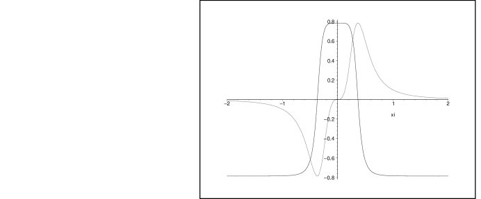
Figure 1: Two solutions of (43) in the light-cone vicinity.

Hence one may treat them as some “potentials” for the local coordinates of GCS $(u=\Re\pi^{1},v=\Im\pi^{1})$. The character of these solutions should be discussed elsewhere.

Conclusion

1. My purpose was to summarize in this work my last results published presently in e-arXiv. We could not treat, of course, these results as finally established. But I think that the natural character of the assumptions which I put in the base of this theory and the mathematically simple method of derivation of the fundamental “field shell” equations, will be attractive for future investigations.

2. The concept of “super-relativity” [11, 22, 25, 26] is in fact some kind of “hybridization” of internal and space-time symmetries. The distinction in kind between SUSY where a priori exists the extended space-time - “super-space” and my approach is that dynamical space-time arises under “yes/no” objective quantum measurement. This “measurement” is represented by the covariant differentiation of $SU(N)$ local dynamical variables in the functional quantum phase space $CP(N-1)$ along the curve of evolution.

References

- [1] M.V.Berry, “The Quantum Phase, Five Years After”, Reprents collection, “Geometric Phases in Physics” (A. Shapere and F. Wilczek, Eds.), World Scientific, Singapore, 1989.
- [2] J.Anandan, Y.Aharonov, Phys.Rev. D38, (6) 1863 (1988).
- [3] Y.Aharonov, et al, arXive: quant-ph/9708043.
- [4] M.V.Berry, Proc.R.Soc.Lond.A 414, 31 (1987).
- [5] F. Wilczek, A.Zee, Phys.Rev.Lett.38, (24) 2111 (1984).
- [6] J.Anandan, L.Stodolsky, arXive: quant-ph/9908046.
- [7] P.A.M. Dirac, Lectures on quantum field theory, New York, Yeshiva University, 1967.
- [8] P.A.M. Dirac, Nuovo Cimento, Suppl. 6, 322 (1957).
- [9] P.Leifer, arXive: physics/0601201.
- [10] V.I.Arnol’d, Mathematical Method of Classical Mechanics (Spring-Verlag, Berlin, 1978).
- [11] P.Leifer, Found. Phys. 27, (2) 261 (1997).
- [12] S.Kobayashi, K.Nomizu, Foundations of Differential Geometry, (Interscience Publisher, New York-London-Sydney, 1969).
- [13] R.Penrose, The Road to Reality, Alfred A.Knopf, New-York, (2005).
- [14] A.Einstein, Ann. Phys. 17, 891 (1905).
- [15] A.Einstein, Ann. Phys. 49, 769 (1916).
- [16] T.D.Newton and E.P.Wigner, Rev. Mod. Phys., 21, 400 (1949).
- [17] G.C.Hegerfeldt, Phys.Rev.D10, 3320 (1974).
- [18] Y.Aharonov, et al, Phys.Rev.A57, 4130 (1998).
- [19] P.Leifer, arXive: gr-qc/0503083.
- [20] P.Leifer and L.P.Horwitz, arXive: gr-qc/0505051, V.2.
- [21] P.Leifer, arXive: physics/0611179.
- [22] P.Leifer, arXive: physics/0612249.
- [23] M.V.Berry, Lectures on Quantum Adiabatic Anholonomy, (1990).
- [24] C.W.Misner, K.S.Thorne, J.A.Wheeler,Gravitation, W.H.Freeman and Company, San Francisco, 1973.
- [25] P.Leifer, Found.Phys.Lett., 18, (2) 195 (2005).
- [26] P.Leifer, JETP Letters, 80, (5) 367 (2004).