A Comparison of Two Shallow Water Models with Non-Conforming Adaptive Grids: classical tests

Abstract

In an effort to study the applicability of adaptive mesh refinement (AMR) techniques to atmospheric models an interpolation-based spectral element shallow water model on a cubed-sphere grid is compared to a block-structured finite volume method in latitude-longitude geometry. Both models utilize a non-conforming adaptation approach which doubles the resolution at fine-coarse mesh interfaces. The underlying AMR libraries are quad-tree based and ensure that neighboring regions can only differ by one refinement level. The models are compared via selected test cases from a standard test suite for the shallow water equations. They include the advection of a cosine bell, a steady-state geostrophic flow, a flow over an idealized mountain and a Rossby-Haurwitz wave. Both static and dynamics adaptations are evaluated which reveal the strengths and weaknesses of the AMR techniques. Overall, the AMR simulations show that both models successfully place static and dynamic adaptations in local regions without requiring a fine grid in the global domain. The adaptive grids reliably track features of interests without visible distortions or noise at mesh interfaces. Simple threshold adaptation criteria for the geopotential height and the relative vorticity are assessed.

1 Introduction

Simulating the climate is a grand challenge problem requiring multiple, century-long integrations of the equations modeling the Earth’s atmosphere. Consequently, grid resolutions in atmospheric climate models are much coarser than in numerical weather models, where accurate predictions are limited to about ten days. However, it has been recognized that localized flow structures, like hurricanes, may play an important role in obtaining the correct climate signal. In particular, there exists a requirement for localized mesh refinement in regional climate modeling studies. It is also conjectured, at this time, that the lack of resolution in the tropics is the cause of the inability of most climate models to capture the statistical contribution of extreme weather events.

While mesh adaptation is a mature field in computational fluid dynamics, currently, the only fully operational adaptive weather and dispersion model is OMEGA (bacon:2000, ; Gopalakrishnan:2002in, ). The latter is based on the finite-volume approach and uses conforming Delaunay meshes that are locally modified and smoothed. Researchers involved in hurricane or typhoon predictions where amongst the very first to experiment with variable resolutions in atmospheric models. The preferred method consisted of nesting finer meshes statically into coarser ones (Kurihara:1979zv, ; Kurihara:1980jj, ). Nesting is a wide spread technique in current models, especially mesoscale models, to achieve high resolutions (Frohn:2002zp, ) in local regions. Truly adaptive models were first developed by Skamarock:1989ya , Skamarock:1993mk and Dietachmayer:1992tg . Skamarock:1993mk based their adaptive mesh refinement (AMR) strategy on a truncation error estimate (Skamarock:1989gy, ). Continuing in the realm of second order conforming methods Iselin:2002ff developed a dynamically adaptive Multidimensional Positive Definite Advection Transport Algorithm (MPDATA) (Iselin:2005ma, ). MPDATA was thoroughly reviewed in Smolarkiewicz:2006ko because of its various numerical qualities. The discussion addressed generalized space-time coordinates that enable continuous mesh deformations (Prusa:2003vs, ) as well as the generalization of MPDATA to unstructured grids (Smolarkiewicz:2005ih, ). Recently, adaptive schemes on the sphere were also discussed by Jablonowski:2004fa , laeuter:2004 , behrens:2005 and laeuter:2006 where only Jablonowski:2004 utilizes a non-conforming approach. A review of adaptive methods in atmospheric modeling is given in behrens:2006 .

It is recognized that high-order spatial resolution is necessary in climate modeling. To paraphrase Boyd:2004lc , spectral methods like continuous Galerkin (CG) or discontinuous Galerkin (DG) are blessedly free of the spurious wave dispersion induced by low-order methods. The corresponding reduction in grid points directly lowers the amount of costly column physics evaluations. Multiple efforts to include conforming mesh refinement techniques in models with high-order numerical methods were initiated Giraldo:2000nu , Fournier:2004wk , Giraldo:2005yj , Giraldo:2006gw and Rosenberg:2006zs . However, supporting conforming adaptive meshes has negative effects on the Courant-Friedrich-Levy (CFL) stability condition. One solution is to consider non-conforming elements or blocks.

In this paper two adaptive mesh techniques for 2D shallow water flows on the sphere are compared. In particular, the study focuses on the characteristics of the AMR approach in the cubed-sphere spectral element model (SEM) by St-Cyr:2006xf and compares it to the adaptive finite volume (FV) method by Jablonowski:2006 . Both SEM and FV are AMR models of the non-conforming type. A thorough study of the dynamically adaptive FV scheme based on quadrilateral control volumes can also be found in Jablonowski:2004fa and Jablonowski:2006b . In particular, 2D shallow water and 3D primitive-equation numerical experiments were conducted using a latitude-longitude grid on the sphere. This adaptive model is built upon the finite volume technique by Lin:1996 and Lin:1997 . The spectral element model is based on the ideas of Patera:1984uq . The non-conforming treatment follows the interpolation procedure by Fischer:2002sx . The spectral element method was originally developed for incompressible fluid flows. Meanwhile, it has been adapted by many authors (Haidvogel:1997kx, ; Taylor:1997vn, ; Giraldo:2001ys, ; Thomas:2002ti, ) for global atmospheric and oceanic simulations.

The paper is organized as follows. In Section 2 the shallow water equations are introduced which are the underlying equation for our model comparison. Both models SEM and FV are briefly reviewed in Section 2. This includes a discussion of the adaptive mesh approach for the spectral elements in SEM and the latitude-longitude blocks in FV. In Section 4 the characteristics of the AMR techniques are tested using selected test cases from the Williamson:1992ts shallow water test suite. They include the advection of a cosine bell, a steady-state geostrophic flow, a flow over a mountain and a Rossby-Haurwitz wave. The findings are summarized in Section 5.

2 Shallow water equations

The shallow water equations have been used as a test bed for promising numerical methods by the atmospheric modeling community for many years. They contain the essential wave propagation mechanisms found in atmospheric General Circulation Models (GCMs). The linearized primitive equations yield a series of layered shallow water problems where the mean depth of each layer is related to the maximum wave speed supported by the medium. These are the fast-moving gravity waves and nonlinear Rossby waves. The latter are important for correctly capturing nonlinear atmospheric dynamics. The governing equations of motion for the inviscid flow of a free surface are given by

$$\frac{\partial\,\mathbf{v}}{\partial t}+(f+\zeta)\>{\bf k}\times\mathbf{v}+\frac{1}{2}\mathbf{\nabla}\left(\mathbf{v}\cdot\mathbf{v}\right)+\mathbf{\nabla}(\Phi+\Phi_{s}) =0$$ (1)

$$\frac{\partial\,\Phi}{\partial t}+\mathbf{\nabla\cdot}(\Phi\mathbf{v}) =0$$ (2)

where $t$ is the time, $\Phi=gh$ symbolizes the geopotential, $h$ is the height above sea level and $g$ denotes the gravitational acceleration. Furthermore, $\Phi_{s}=gh_{s}$ is the surface geopotential, $h_{s}$ symbolizes the height of the orography, $\mathbf{v}$ stands for the horizontal velocity vector, ${\bf k}$ denotes the radial outward unit vector, and $f$ and $\zeta$ are the Coriolis parameter and relative vorticity, respectively. $\mathbf{\nabla}$ indicates the horizontal gradient operator, whereas $\mathbf{\nabla\cdot}$ stands for the horizontal divergence operator. The momentum equation (1) is written in its vector-invariant form.

3 Description of the adaptive shallow water models

The spectral element method (SEM) is a combination of ideas coming from the finite-element method and of the spectral method. The order of accuracy is determined by the degree of the local basis functions within a finite element. The basis consists of Lagrange polynomials passing through Gauss-Legendre-Lobatto (GLL) or Gauss-Legendre (GL) quadrature points facilitating greatly the evaluation of the integrals appearing in a weak formulation. For the tests here, fifth degree basis functions for scalars are employed which utilize $6\times 6$ GL quadrature points per spectral element. The SEM grid is based on a projection of a cube inscribed into a sphere (Sadourny:1972xo ), a so-called cubed-sphere grid which consists of 6 faces. These are further subdivided into spectral elements quadrangles which are evenly distributed over the surface of the sphere in the non-adapted case. Note that the numerical approach in SEM is non-monotonic and does not conserve mass. Nevertheless, the variation in the total mass is small over typical forecast periods of two weeks.

This is in contrast to the monotonic and mass-conservative FV model which was originally developed by Lin:1997 . It utilizes the third order Piecewise Parabolic Method (PPM) (Colella:1984hi, ) which was first designed for compressible fluids with strong shocks. The PPM algorithm applies monotonicity constraints that act as a nonlinear scale-selective dissipation mechanism. This dissipation primarily targets the flow features at the smallest scales.

Both shallow water models are characterized in more detail below. In particular, the individual adaptive mesh approaches are described which implement adaptations in the horizontal directions. The time step, on the other hand, is not adapted, except for selected advection tests. Therefore, the chosen time step must be numerically stable on the finest grid in an adapted model run.

3.1 Spectral element (SEM) shallow water model

3.1.1 Curvilinear coordinates: cubed sphere

The flux form shallow-water equations in curvilinear coordinates are described in Sadourny:1972xo . Let $\mathbf{a}_{1}$ and $\mathbf{a}_{2}$ be the covariant base vectors of the transformation between inscribed cube and spherical surface. The metric tensor of the transformation is defined as $G_{ij}\equiv\mathbf{a}_{i}\cdot\mathbf{a}_{j}$. Covariant and contravariant vectors are related through the metric tensor by $u_{i}=G_{ij}u^{j}$ and $u^{i}=G^{ij}u_{j}$, where $G^{ij}=(G_{ij})^{-1}$ and $G=\det(G_{ij})$. The six local coordinate systems $(x^{1},x^{2})$ are based on an equiangular central projection, $-\pi/4\leq x^{1},x^{2}\leq\pi/4$. The metric tensor for all six faces of the cube is

$$G_{ij}=\frac{1}{r^{4}\cos^{2}x^{1}\,\cos^{2}x^{2}}\,\left[\begin{array}[]{cc}1+\tan^{2}x^{1}&-\tan x^{1}\,\tan x^{2}\\ -\tan x^{1}\,\tan x^{2}&1+\tan^{2}x^{2}\end{array}\right]$$ (3)

where $r=(1+\tan^{2}x^{1}+\tan^{2}x^{2})^{1/2}$ and $\sqrt{G}=1/r^{3}\,\cos^{2}x^{1}\,\cos^{2}x^{2}$.

The shallow water equations are written in curvilinear coordinates using the following definitions for divergence and vorticity

$$\nabla\cdot{\bf v}\equiv\frac{1}{\sqrt{G}}\left[\frac{\partial}{\partial x^{i}}\;(\;\sqrt{G}\;u^{i}\;)\right],\quad\zeta\equiv\frac{\epsilon_{ij}}{\sqrt{G}}\frac{\partial u_{j}}{\partial x^{i}}=\frac{1}{\sqrt{G}}\left[\frac{\partial u_{2}}{\partial x^{1}}-\frac{\partial u_{1}}{\partial x^{2}}\right]$$

and replacing them in (2). In their contravariant form the equations are

$$\frac{\partial u^{i}}{\partial t}+G^{ij}\left[\frac{\partial}{\partial x^{j}}(u^{k}u_{k})+\frac{\partial\Phi}{\partial x^{j}}+\sqrt{G}\,\epsilon_{jk}u^{k}(f+\zeta)\right] =0,$$ (4)

$$\frac{\partial\Phi}{\partial t}+u^{j}\frac{\partial\Phi}{\partial x^{j}}+\frac{\Phi}{\sqrt{G}}\frac{\partial}{\partial x^{j}}(\sqrt{G}u^{j}) =0$$ (5)

where the Einstein summation convention is used for repeated indices. Additional information on the equation set can also be found in Nair:2005aj .

3.1.2 Spatial and temporal discretization

The equations of motion are discretized in space using the ${\mathbb{P}}_{N}-{\mathbb{P}}_{N-2}$ spectral element method as in Thomas:2002ti . The cubed-sphere is partitioned into $K$ elements $\Omega^{k}$ in which the dependent and independent variables are approximated by tensor-product polynomial expansions. The velocity on element $\Omega^{k}$ is expanded in terms of the $N$-th degree Lagrangian interpolants $h_{i}$

$${\bf v}_{h}^{k}({\bf x})=\sum_{i=0}^{N}\sum_{j=0}^{N}\>{\bf v}^{k}_{ij}\>h_{i}(\xi^{k}({\bf x}))\>h_{j}(\eta^{k}({\bf x}))$$ (6)

and the geopotential is expanded on the same element using the $(N-2)$–th degree interpolants $\tilde{h}_{i}$

$${\Phi}_{h}^{k}({\bf x})=\sum_{i=1}^{N-1}\sum_{j=1}^{N-1}\>{\Phi}^{k}_{ij}\>\tilde{h}_{i}(\xi^{k}({\bf x}))\>\tilde{h}_{j}(\eta^{k}({\bf x}))$$ (7)

where ${\bf x}\rightarrow(\xi^{k}({\bf x}),\eta^{k}({\bf x}))$ is an affine transformation from the element $\Omega^{k}$ on the cubed sphere to the reference element $[-1,1]\times[-1,1]$ pictured in Fig. 1. A weak Galerkin formulation results from the integration of the equations with respect to test functions and the direct evaluation of inner products using Gauss-Legendre and Gauss-Lobatto-Legendre quadrature. The positions of the corresponding GL and GLL quadrature points within each spectral element with mapped coordinates $\xi$ and $\eta$ are depicted in Fig. 1. The GLL points for the co-located velocity components are marked by the circles, the open squares point to the GL points for scalars. The polynomial degrees are 7 and 5, respectively. An overview of the chosen parameters and base resolutions for the present study is also given in Table 1.

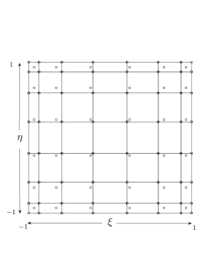
Fig. 1: Positions of the GLL (circles) and GL (open squares) quadrature points on the spectral reference element with mapped coordinates $\xi$ and $\eta$. The polynomial degrees are 7 (GLL velocity points) and 5 (GL scalar points).

Table 1: Overview of the resolutions in SEM.

# Elements	Total # of	# GL points	# GLL points	Approximate
per cubed face	elements	per element	per element	resolution
$3\times 3$	54	$6\times 6$	$8\times 8$	$5^{\circ}\times 5^{\circ}$
$4\times 4$	96	$6\times 6$	$8\times 8$	$3.2^{\circ}\times 3.2^{\circ}$
$6\times 6$	216	$6\times 6$	$8\times 8$	$2.5^{\circ}\times 2.5^{\circ}$

$C^{0}$ continuity of the velocity is enforced at inter-element boundaries sharing Gauss-Lobatto-Legendre points and direct stiffness summation (DSS) is then applied (Tufo:1998ey, ; Deville:2002fn, ). The advection operator in the momentum equation is expressed in terms of the relative vorticity and kinetic energy, whereas the continuity equation relies on the velocity form. Wilhelm:uo have shown that the rotational form of the advection operator is stable for the ${\mathbb{P}}_{N}-{\mathbb{P}}_{N-2}$ spectral element discretization. A standard Asselin-Robert filtered leap-frog discretization is employed for integrating the equations of motion in time. More advanced options, that are tailored for AMR based on the ideas in St-Cyr:2005ur , will be described in St-Cyr:2006xf . Since a spectral basis is employed on each element, the spectrum of the advective operators must be corrected using a $2/3$ rule similar to what is employed in global pseudo spectral models. A Boyd-Vandeven filter (Vandeven:1991ef, ; Boyd:1996hn, ) was used during the adaptive numerical simulations that removes the last third of the spectrum.

3.1.3 Non-conforming spectral elements

The positions of the collocation points at the boundaries of non-conforming spectral elements do not coincide and a procedure is required to connect neighboring elements. Several techniques are available including mortars (Mavriplis:1989xe, ; Feng:2002uq, ) and interpolations (Fischer:2002sx, ). Here, interpolations are used. The true unknowns at a boundary belong to the master coarse element and are passed to the refined slave elements by the following procedure. From Eq. (6), at one of the element boundaries $\Gamma_{km}=\Omega_{k}\cap\Omega_{m}$ with $\xi^{k}=\xi^{m}=1$, the trace of the solution is

$${\bf v}({\bf x}(\xi^{k},\eta^{k}))_{h}^{k}|_{\Gamma_{km}}={\bf v}_{h}^{k}({\bf x}(1,\eta^{k}))=\sum^{N}_{j=0}{\bf v}^{k}_{Nj}h_{j}(\eta^{k})$$ (8)

where $h_{j}$ are the Lagrange interpolants defined at the GLL points. To interpolate the master solution to the slave edge, a mapping is created from the master reference element relative to the slave’s reference element. Let $\eta^{l}_{m}$ denote this mapping, then

$$\eta^{l}_{m}(\eta):=\frac{\eta}{2^{l}}+\frac{2m-1}{2^{l}}-1$$ (9)

where $m\in[1,2^{l}]$ is the slave face number and $l$ is the number of the refinement level. This spatial refinement strategy is called $h$–refinement which is in contrast to increasing the order of the polynomials ($p$–refinement).

Interpolations can be expressed in matrix form as

$$\left[J^{l}_{m}\right]_{ij}=h_{j}(\eta^{l}_{m}(\xi_{i}))$$ (10)

where $\{\xi_{i}\}^{N}_{i=0}$ are the Gauss-Legendre-Lobatto points used in the quadrature and in the collocation of the dependent variables. If ${\bf v}^{k}$ are the unknowns on the edge of the master element, then $J^{l}_{m}{\bf v}^{k}$ represents the master element contributions passed to the slave elements. Assembly of the global spectral element matrix is not viable on today’s computer architectures with distributed memory. Instead, the action of the assembled matrix on a vector is performed with the help of DSS. For $A$, a matrix resulting from the spectral element discretization of a differential operator, defined for the true degrees of freedom and $A_{L}$, the block diagonal matrix of the individual local unassembled contributions of each element as if they were disjoint, the DSS for conforming elements is represented by

$$v^{T}Au=v^{T}Q^{T}A_{L}Qu$$ (11)

where $Q$ is a Boolean rectangular matrix representing the scattering of the true degrees of freedom to the unassembled blocks (one block in $A_{L}$ per element). A non-conforming formulation can be obtained by replacing the scattering Boolean matrices $Q$ with $Q=J_{L}\tilde{Q}$

$$v^{T}Au=v^{T}(\tilde{Q}^{T}J^{T}_{L})A_{L}(J_{L}\tilde{Q})u\mbox{.}$$ (12)

The block diagonal matrix $J_{L}$ consist of the identity where the interfaces between elements match and of the interpolation matrix (10) where interfaces are non-conforming. To facilitate time-stepping procedures, the matrix must be lumped by summing rows in the mass matrix (Quarteroni:1997kw, ). Let $L(A)$ represent the lumping operation. Lumping the global matrix $A$ is equivalent to lumping the local matrix $J^{T}_{L}A_{L}J_{L}$ and it can be shown that

$$L(A)=L(\tilde{Q}^{T}J^{T}_{L}A_{L}J_{L}\tilde{Q})=\tilde{Q}^{T}L(J^{T}_{L}A_{L}J_{L})\tilde{Q}.$$ (13)

3.1.4 Adaptation principle

The adaptation algorithm developed here is parallel and usable on distributed memory computers. The cubed sphere is initially tiled with an uniform, low resolution, mesh and each element represents the root of a quad-tree. While a quad-tree is a natural description for 2-dimensional mesh refinement, the six faces of the cubed-sphere geometry necessitates a graph data structure. For the quad-trees, a set of simple bit manipulation subroutines are used to provide inheritance information. A graph data structure which describes the connection between the roots and leaves of each quad-tree is also maintained. To simplify the interface management, neighboring elements are restricted to be at most one level of refinement apart. When elements are marked for refinement, a parallel procedure verifies that a compatible quad-tree refinement exists, with respect to all the roots and the interface restriction. The communication package is properly modified to enable correct inter-element communications related to the DSS procedure. This was greatly simplified by replacing the graph-based communication package in the model by the more generic one developed by Tufo:1998ey . If a load imbalance is detected then the partitioning algorithm is invoked and elements are migrated to rebalance the workload on each processor. Apart from the Message Passing Interface (MPI) library, the graph partitioning tool ParMeTiS(Karypis:2002yo, ) and the generic DSS libraries, no other specialized high-level library is used. The non-adapted spectral element model also supports an efficient space-filling curve loadbalancing approach (dennis:03, ) which we plan to use in the adaptive model for future simulations.

3.2 Finite volume (FV) shallow water model

3.2.1 Model description

The adaptive finite volume model is built upon the advection algorithm by Lin:1996 and its corresponding shallow water system (Lin:1997, ). The FV shallow water model is comprised of the momentum equation and mass continuity equation as shown in Eqns. (1) and (2). Here the flux-form of the mass conservation law and the vector-invariant form of the momentum equation are selected. In addition, a divergence damping term is added to the momentum equation.

The finite-volume dynamical core utilizes a flux form algorithm for the horizontal advection processes, which, from the physical point of view, can be considered a discrete representation of the conservation law in finite-volume space. However, from the mathematical standpoint, it can be viewed as a numerical method for solving the governing equations in integral form. This leads to a more natural and often more precise representation of the advection processes, especially in comparison to finite difference techniques. The transport processes, e.g. for the height $h=\Phi/g$ of the shallow water system, are modeled by fluxes into and out of the finite control-volume where volume-mean quantities are predicted

$$\bar{h}_{i,j}^{n+1} = \bar{h}_{i,j}^{n}-\frac{\Delta t}{a\,\cos\phi_{j}\,\Delta\lambda_{i}}\>\big{(}F_{i+\frac{1}{2},j}-F_{i-\frac{1}{2},j}\big{)}$$ (14)

$$\quad\;\,\,-\frac{\Delta t}{a\,\cos\phi_{j}\,\Delta\phi_{j}}\>\big{(}\cos\phi_{j+\frac{1}{2}}\,G_{i,j+\frac{1}{2}}\,-\,\cos\phi_{j-\frac{1}{2}}\,G_{i,j-\frac{1}{2}}\big{)}\mbox{.}$$

Here, the overbar $\bar{()}$ indicates the volume-mean, $F$ and $G$ denote the time-averaged 1D numerical fluxes in longitudinal and latitudinal direction which are computed with the upstream-biased and monotonic PPM scheme (see also carpenter:90 and nair:02 ). $\Delta t$ symbolizes the time step, $a$ stands for the radius of the Earth, the indices $i$ and $j$ point to grid point locations in the longitudinal ($\lambda$) and latitudinal ($\phi$) direction and the index $n$ marks the discrete time level. In addition, $\Delta\lambda_{i}=(\lambda_{i+\frac{1}{2}}-\lambda_{i-\frac{1}{2}})$ and $\Delta\phi_{i}=(\phi_{j+\frac{1}{2}}-\phi_{j-\frac{1}{2}})$ represent the longitudinal and latitudinal grid distances measured in radians.

The advection algorithm shown in Eq. (14) is the fundamental building block of the horizontal discretization in the FV shallow water model. It is not only used to predict the time evolution of the mass (Eq. (2)), but also determines the absolute vorticity fluxes and kinetic energy in the momentum equation. Further algorithmic details of the shallow water code are described in Lin:1997 who also discussed the staggered Arakawa C and D grid approach utilized in the model.

3.2.2 Block-structured adaptive mesh approach

The AMR design of the FV shallow water model is built upon a 2D block-structured data configuration in spherical coordinates. The concept of the block data structure and corresponding resolutions is fully described in Jablonowski:2006 . In essence, a regular latitude-longitude grid is split into $B_{y}\times B_{x}$ non-overlapping spherical blocks that span the entire sphere. Each block is logically rectangular and comprises a constant number of $N_{y}\times N_{x}$ grid points in latitudinal and longitudinal direction. If, for example, $6\times 9$ grid points per block are selected with $B_{y}\times B_{x}=6\times 8$ blocks on the sphere then the configuration corresponds to a $5^{\circ}\times 5^{\circ}$ uniform mesh resolution. Here, we use such an initial configuration for selected test cases in Section 4. All blocks are self-similar and split into four in the event of refinement requests, thereby doubling the spatial resolution. Coarsenings reverse this refinement principle. Then four “children” are coalesced into a single self-similar parent block which reduces the grid resolution in each direction by a factor of 2. As in SEM neighboring blocks can only differ by one refinement level. This leads to cascading refinement areas around the finest mesh region. In addition, the blocks adjacent to the poles are kept at the same refinement level due to the application of a fast Fourier transform (FFT) filter in longitudinal direction for nonlinear flows.

The FV model supports static and dynamic adaptations which are managed by an adaptive block-structured grid library for parallel processors (oehmke:01, ; oehmke:04, ). This library utilizes a quad-tree representation of the adapted grid which is similar to the adaptive mesh technique in SEM. The communication on parallel computer architectures is performed via MPI. Our load-balancing strategy aims at assigning an equal workload to each processor which is equivalent to an equal number of blocks in the FV shallow water model. No attempt is made to keep geographical regions on the same processor. This can be achieved by a space-filling curve load-balancing strategy as in dennis:03 which reduces the communication overhead. Such an approach is the subject of future research. The refinement criteria are user selected. In particular, simple geopotential height thresholds or vorticity-based criteria are assessed for our dynamic adaptation tests. For static adaptations though, we place the fine-grid nests in pre-determined regions like mountainous areas or geographical patches of interest.

Each block is surrounded by ghost cell regions that share the information along adjacent block interfaces. This makes each block independent of its neighbors since the solution technique can now be individually applied to each block. The ghost cell information ensures that the requirements for the numerical stencils are satisfied. The algorithm then loops over all available blocks on the sphere before a communication step with ghost cell exchanges becomes necessary. The number of required ghost cells highly depends on the numerical scheme. Here, three ghost cells in all horizontal directions are needed which are kept at the same resolution as the inner domain of the block. The consequent interpolation and averaging techniques are further described in Jablonowski:2004fa and Jablonowski:2006 .

The time-stepping scheme is explicit and stable for zonal and meridional Courant numbers $|$CFL$|<1$. This restriction arises since the semi-Lagrangian extension of the Lin:1996 advection algorithm is not utilized in the AMR model experiments. This keeps the width of the ghost cell regions small, but on the other hand requires small time steps if high wind speeds are present in polar regions. Then the CFL condition is most restrictive due to the convergence of the meridians in the latitude-longitude grid. Therefore, we restrict the adaptations near the pole to very few (1-2) refinement levels.

The adaptive grids of both models are compared in Fig. 2. Here, an idealized mountain as indicated by the contour lines is refined at the maximum refinement level of 3. This corresponds to the grid resolution $0.625^{\circ}\times 0.625^{\circ}$ in the finest adaptation region. The adaptive elements (SEM) and blocks (FV) overlay the sphere. The differences between the two adaptive meshes are clearly visible. The SEM model (Fig. 2a) utilizes a non-orthogonal cubed-sphere geometry and places the refined spectral elements across an edge of two cubed-sphere faces. The FV model (Fig. 2b) is formulated on a latitude-longitude grid. This leads to orthogonal blocks which are closely spaced in polar regions.

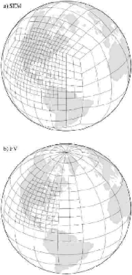
Fig. 2: Adaptive grids on the sphere in (a) SEM and (b) FV. The adapted elements on the cubed-sphere (SEM) and adapted blocks in latitude-longitude geometry (FV) refine an idealized mountain as indicated by the contour lines.

4 Numerical experiments

For our AMR model intercomparison, we select test cases with increasing complexity from the standard Williamson:1992ts shallow water test suite. The Williamson:1992ts test suite assesses scenarios that are mainly characterized by large-scale smooth flow fields. Among them are the passive advection of a cosine bell (test case 1), a steady-state geostrophic flow at various rotation angles (test case 2), a flow over an idealized mountain (test case 5) and a Rossby-Haurwitz wave with wavenumber 4 (test case 6). Our discussion of the adaptive models is focused on these tests. Both static and dynamic refinement areas are addressed that highlight the strengths and weaknesses of the two AMR approaches.

Some basic statistics of the adaptive simulations can be found in Table 2. The table lists not only the test case numbers with corresponding rotation angles $\alpha$ and base resolutions, but also gives information on the AMR approach, the number of refinement levels, the time steps as well as the number of adapted elements (SEM) and blocks (FV) at certain snapshots in time. Note that the time steps are not optimized for performance. Rather they are selected to guarantee numerical stability.

Table 2: Statistics for the adaptive SEM and FV simulations.

Test		Base	# Ref.		SEM			FV
case	$\alpha$	resolution	level	AMR	$\Delta t$ (s)	# Elements		$\Delta t$ (s)	# Blocks
1	$45^{\circ}$	$5^{\circ}\times 5^{\circ}$	3	dynamic	10	322 (day 9)		adaptive	201 (day 9)
1	$90^{\circ}$	$5^{\circ}\times 5^{\circ}$	3	dynamic	10	242 (day 3)		adaptive	480 (day 3)
2	$45^{\circ}$	$2.5^{\circ}\times 2.5^{\circ}$	2	static	10	324		200	288
5		$5^{\circ}\times 5^{\circ}$	3	dynamic	20	1448 (day 15)		138	744 (day 15)
6		$2.5^{\circ}\times 2.5^{\circ}$	1	static	15	312		225	288
6		$3.2^{\circ}\times 3.2^{\circ}$	1	static	15	176		–	–

The model results are typically evaluated via normalized $l_{1}$, $l_{2}$ and $l_{\infty}$ error norms. The definitions of the norms are given in Williamson:1992ts . For the adaptive FV shallow water model the computation of the norms is also explained in Jablonowski:2006 .

4.1 Passive advection of a cosine bell

We start our intercomparison of the two AMR approaches with the traditional solid body rotation of a cosine bell around the sphere (see test case 1 in Williamson:1992ts for the initial conditions). This test evaluates the advective component of the numerical method in isolation. It challenges the spectral element method of SEM due to possible over- and undershoots of the transported feature. They are due to the so-called Gibbs phenomenon which is characteristic for spectral approaches (Gibbs:1899fk, ; Vandeven:1991ef, ; Boyd:1996hn, ). Several values for the rotation angle $\alpha$ can be specified. It determines the angle between the axis of the solid body rotation and the poles in the spherical coordinate system. Here, we mainly report results for $\alpha=45^{\circ}$ which advects the cosine bell slantwise over four corner points and two edges of the cubed-sphere. In addition, results for $\alpha=0^{\circ}$ (transport along the equator) and $\alpha=90^{\circ}$ (transport over the poles) are discussed. The length of the integration is 12 days which corresponds to one complete revolution of the cosine bell around the sphere. The base resolution for both shallow water models is a $5^{\circ}\times 5^{\circ}$ coarse mesh with additional initial refinements surrounding the cosine bell. In particular, the base resolution in SEM is represented by $54$ elements (see Table 1) whereas the adaptations in FV start from $6\times 8$ initial blocks. We test the refinement levels 1, 2, 3 and 4 which are equivalent to the resolutions $2.5^{\circ}\times 2.5^{\circ}$, $1.25^{\circ}\times 1.25^{\circ}$, $0.625^{\circ}\times 0.625^{\circ}$ and $0.3125^{\circ}\times 0.3125^{\circ}$ within the refined areas. Note that these grid spacings only represent approximate resolutions for SEM because of the clustering of the collocation points near the element boundaries (see Fig. 1).

In both models we refine the grid if the geopotential height field of the cosine bell exceeds $h\geq 53$ m. This value corresponds to approximately 5% of the initial peak value with $h_{max}=1000$ m. Of course, other refinement thresholds are also feasible. The threshold has been chosen since the refined area now tightly surrounds the cosine bell in the regular latitude-longitude grid (model FV). In SEM though, the adaptations are padded by a one-element wide halo. This leads to a broader refined area in comparison to FV but less evaluations of the refinement criterion. For the FV model, the refinement criterion is evaluated at every time step. The grid is refined up to the maximum refinement level whenever the criterion is met. Grid coarsenings are invoked after the cosine bell left the refined area and consequently, the criterion is no longer fulfilled. The time steps in the FV simulations are variable and match a CFL stability criterion of $|$CFL$|\leq 0.95$ at the finest refinement level. This setup corresponds exactly to the adaptive advection experiments with FV in Jablonowski:2006 . For the SEM model, the time-step is constant and restricted by the CFL number computed on the finest grid.

Figure 3 shows snapshots of the cosine bell with rotation angle $\alpha=45^{\circ}$ and three refinement levels ($0.625^{\circ}\times 0.625^{\circ}$) at day 3, 6, 9 and 12. The SEM model with its refined spectral elements on the cubed sphere is depicted in the left column (Fig. 3a-d), the right column (Fig. 3e-g) displays the FV model with its block-structured latitude-longitude grid. Note that each spectral element (SEM) contains additional $6\times 6$ GL grid points, whereas each block (FV) consists of $6\times 9$ grid points in the latitudinal and longitudinal direction, respectively.

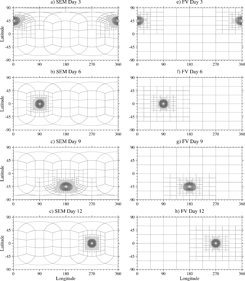
Fig. 3: Snapshots of the cosine bell (test case 1) with rotation angle $\alpha=45^{\circ}$ and three refinement levels at day 3, 6, 9 and 12. The finest grid spacing is $0.625^{\circ}\times 0.625^{\circ}$, the adapted spectral elements (SEM) and blocks (FV) are overlaid. Left column (a-d) shows the SEM model, right column (e-h) depicts the FV model. The contour interval is 100 m, the zero contour is omitted.

In both models the initial state (not shown) resembles the final state (day 12) very closely. It can clearly be seen that the adapted grids of both models reliably track the the cosine bell without visible distortion or noise.

The errors can be further assessed in Fig. 4 which shows the time traces of the normalized $l_{1}$, $l_{2}$ and $l_{\infty}$ norms of the geopotential height field for rotation angle $\alpha=45^{\circ}$. At this rotation angle the errors in SEM are an order of magnitude smaller than the errors in FV. This is mainly due to the operator-splitting approach in FV which produces the maximum error at $\alpha=45^{\circ}$. It is apparent that SEM transports the cosine bell rather smoothly across the corners of the cubed mesh. The errors in FV are considerably lower for rotation angle $\alpha=0^{\circ}$. This is shown in Table 3 that documents the $\alpha=0^{\circ}$ normalized height errors as well as the absolute maximum and minimum of the height field after one full revolution for the refinement levels 1 through 4. The errors of both models at any refinement level are now comparable to each other. In addition, the table shows that SEM introduces undershoots during the simulation which are documented by the negative minimum height values $h_{min}$. This is not the case for the monotonic and conservative FV advection algorithm. Here it can also be seen that the maximum height of the cosine bell $h_{max}$ in FV is affected by the monotonicity constraint which acts as a nonlinear dissipation mechanism. It consequently reduces the peak amplitude of the cosine bell, especially at lower resolutions when the bell is not well-resolved. This decrease in maximum amplitude is less profound in SEM.

Fig. 4: Time traces of the normalized $l_{1}$, $l_{2}$ and $l_{\infty}$ geopotential height error norms for the cosine bell advection test (test case 1) with $\alpha=45^{\circ}$. The (a) SEM and (b) FV advection models utilized three refinement levels that correspond to the finest grid resolution $0.625^{\circ}\times 0.625^{\circ}$. Note that the scales in (a) and (b) differ by a factor of 10.

Table 3: Normalized height error norms and characteristics for the advection of a cosine bell (test case 1) after one revolution (day 12) at different refinement levels and rotation angle $\alpha=0^{\circ}$ . The first column indicates the resolution of the grid within the refined area. Both the SEM model (top) and FV model (bottom) are shown.

Resolution	$l_{1}$	$l_{2}$	$l_{\infty}$	$h(m)$ $\max$/$\min$
SEM
$2.5^{\circ}\times 2.5^{\circ}$	0.0503	0.0269	0.0195	991.6/-15.1
$1.25^{\circ}\times 1.25^{\circ}$	0.0085	0.0056	0.0057	997.5/-4.2
$0.625^{\circ}\times 0.625^{\circ}$	0.0019	0.0014	0.0019	999.1/-1.1
$0.3125^{\circ}\times 0.3125^{\circ}$	0.0008	0.0006	0.0015	999.7/-0.9
FV
$2.5^{\circ}\times 2.5^{\circ}$	0.0341	0.0301	0.0317	949.1/0
$1.25^{\circ}\times 1.25^{\circ}$	0.0097	0.0103	0.0150	984.2/0
$0.625^{\circ}\times 0.625^{\circ}$	0.0016	0.0021	0.0044	995.0/0
$0.3125^{\circ}\times 0.3125^{\circ}$	0.0003	0.0005	0.0014	998.4/0

Another snapshot of the cosine bell advection test at day 3 with three refinement levels is shown in Fig. 5. Here, the rotation angle is set to $\alpha=90^{\circ}$ which directs the bell straight over the poles. At day 3, the bell reaches the North Pole and both models refine the grid reliably over this region. Nevertheless, a distinct difference between the two models is the total number of refined elements (SEM) and blocks (FV) needed at high latitudes. While SEM (Fig.  5a) keeps the total number of adapted elements small in the chosen cubed-sphere geometry, the FV model (Fig.  5b) needs to refine a large number of blocks due to the convergence of the meridians in the latitude-longitude mesh. This leads to an increase in the computational workload in the adaptive FV experiment due to the increased number of blocks and small time steps needed in polar regions. In this FV run the time step varies between approximately $\Delta t=600$ s and $\Delta t=10$ s which strongly depends on the position of the cosine bell (Jablonowski:2006, ). The SEM model though utilizes a constant time step of $\Delta t=10$ s. Further statistics for test case 1 are listed in Table 2. In particular, for rotation angle $\alpha=45^{\circ}$ the number of refined blocks in FV is smaller than the number of refined elements in SEM. This effect is mainly due to the additional halo region in SEM.

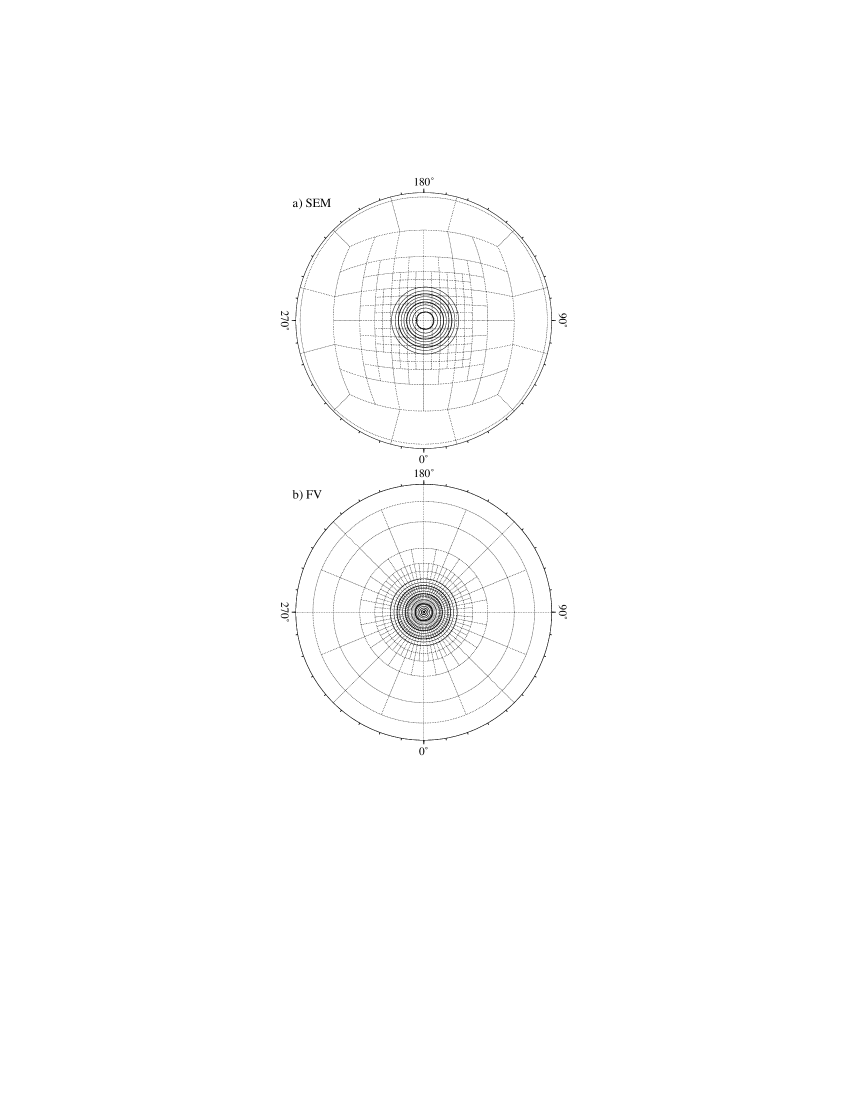
Fig. 5: North-polar stereographic projection of the cosine bell (test case 1) with rotation angle $\alpha=90^{\circ}$ and three refinement levels at day 3 for (a) SEM and (b) FV. The finest grid spacing is $0.625^{\circ}\times 0.625^{\circ}$, the adapted spectral elements (SEM) and blocks (FV) are dotted. The contour interval is 100 m, the zero contour is omitted.

4.2 Steady-state geostrophic flow

Test case $2$ is a steady-state zonal geostrophic flow, representing a balance between the Coriolis and geopotential gradient forces in the momentum equation. The initial velocity field on the sphere is given by

$$u =u_{0}\left(\>\cos\theta\cos\alpha+\cos\lambda\sin\theta\sin\alpha\>\right)$$

$$v =-u_{0}\sin\lambda\sin\alpha~{}.$$

where $\alpha$ is the angle between the axis of solid body rotation and the polar axis. The analytic geopotential field $\Phi=gh$ is specified as

$$\Phi=\Phi_{0}-\left(\>a\Omega u_{0}+\frac{u_{0}^{2}}{2}\>\right)\times\left(\>-\cos\lambda\cos\theta\sin\alpha+\sin\theta\cos\alpha\>\right)^{2}~{}.$$

$a$ is the radius of the earth and $\Omega$ is the rotation rate. Parameter values are specified to be $u_{0}=2\pi a/(12\>{\rm days})$ and $\Phi_{0}=2.94\times 10^{4}$ ${\rm m}^{2}/{\rm s}^{2}$. These fields also represent the analytic solution of the flow. The Coriolis parameter is given by

$$f=2\Omega\left(\>-\cos\lambda\cos\theta\sin\alpha+\sin\theta\cos\alpha\>\>\right).$$

We primarily use this large-scale flow pattern to assess the characteristics of the fine-coarse mesh interfaces in two statically adapted grid configurations. Both models SEM and FV utilize non-conforming meshes with a resolution jump by a factor of two in each direction at the interfaces. Note that the FV model requires interpolations in the ghost cell regions of neighboring blocks whenever the resolution is changed. This is not the case for SEM. In general, inserting a refined patch of elements (SEM) or blocks (FV) in a random location should result in either no changes in the error, if the flow is completely resolved, or in a small decrease in the overall error. Inserting the patch in a strategic location might even lower the error more significantly.

Here, we start our simulations from a uniform $2.5^{\circ}\times 2.5^{\circ}$ base grid which is given by $216$ spectral elements with $6\times 6$ GL points in SEM. In FV, this corresponds to the block data structure consisting of $12\times 16=192$ blocks with $6\times 9$ grid points in latitudinal and longitudinal direction, respectively. Two refinement levels are utilized which lead to the finest mesh spacing $0.625^{\circ}\times 0.625^{\circ}$ in both models.

In the first configuration, a refined patch of size $45^{\circ}\times 30^{\circ}$ (longitudes $\times$ latitudes) is centered at (180^∘E, 45^∘N). This patch spans the domain (157.5^∘E,30^∘N)-(202.5^∘E,60^∘N) which is shown by the dotted contours of the adapted FV blocks in Fig. 6. Here, the geopotential height field of the FV simulation at day 14 is displayed which is visually indistinguishable from the initial state. In the second configuration a patch of identical size is centered at (135^∘E, 30^∘N). This covers the region between (112.5^∘E,15^∘N) - (157.5^∘E,45^∘N) which is characterized by strong gradients in the geopotential height field (see also the discussion in Jablonowski:2004 ). The two locations give insight into the dependency of the errors on the position of the refined patch.

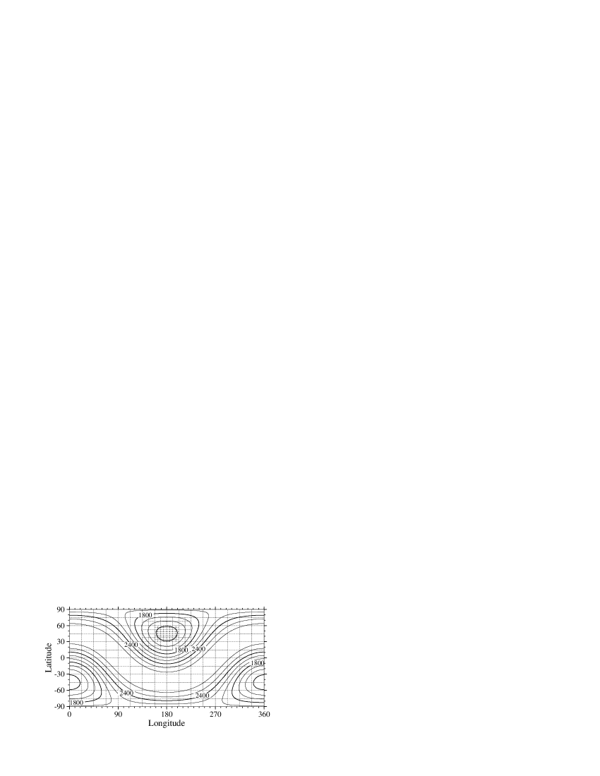
Fig. 6: Geopotential height field for test case 2 with $\alpha=45^{\circ}$ at day 14 as simulated with the FV model. The statically adapted blocks with 2 refinement levels are overlaid (dotted contour). The refined patch is centered at (180^∘E, 45^∘N), the finest grid spacing is $0.625^{\circ}\times 0.625^{\circ}$. The contour interval is 200 m.

Both statically adapted configurations are integrated for $14$ days with $\alpha=45^{\circ}$. As mentioned before this rotation angle represents the most challenging direction for both models due to the choice of the cubed-sphere geometry in SEM and the operator-splitting approach in FV. The results for the $l_{2}$ normalized geopotential height errors for SEM and FV are reported in Fig. 7. It is expected that the errors in SEM are lower than in FV which is confirmed by Figs. 7a-b. This is due to the spectral convergence (SEM) of the smooth solution which is infinitely differentiable. In general, such spectral convergence can not be archived by grid point models which typically exhibit higher error norms. Here it is interesting to note that the two refined patches in SEM lead to a slight decrease in the error in comparison to the uniform-mesh run (Fig. 7a). The errors are independent of the location of the refined area. This is in contrast to the error norms in FV (Fig. 7b). The refined patches introduce slight disturbances of the geostrophic balance and non-divergent wind field which now cause the error norms to increase in comparison to the uniform-mesh run. The increase is sensitive to the location of the refined patch. In particular the errors in FV grow faster if the patch intersects the strong gradient regime in the geopotential height field (centered at (135^∘E, 30^∘N)). Despite this characteristic, the error is still in the expected range for grid point based models, as for example compared to tolstykh:02 . The increase in error is mainly triggered by interpolations in the ghost cell regions (see also Jablonowski:2004fa ; Jablonowski:2006b ) and will be further investigated.

Fig. 7: Time traces of the normalized $l_{2}$ geopotential height error norms for the steady state geostrophic flow (test case 2) with rotation angle $\alpha=45^{\circ}$. Two simulations with static refinement regions centered at (180^∘E, 45^∘) and (135^∘E, 30^∘) are compared to a uniform $2.5^{\circ}\times 2.5^{\circ}$ resolution run. The adaptive (a) SEM and (b) FV model runs start with a $2.5^{\circ}\times 2.5^{\circ}$ base grid with two refinement level (finest grid resolution is $0.625^{\circ}\times 0.625^{\circ}$.)

4.3 Flow over an idealized mountain

Test case 5 of the Williamson:1992ts test suite is a zonal flow impinging on a mountain. The mean equivalent depth of the atmosphere is set to $h_{0}=5960$ m. The mountain height is given by $h_{s}=h_{s_{0}}(1-r/R)$, where $h_{s_{0}}=2000$ m, $R=\pi/9$, and $r^{2}=\min[R^{2},(\lambda-\lambda_{c})^{2}+(\theta-\theta_{c})^{2}]$. The center of the mountain is located at $\lambda_{c}=3\pi/2$ and $\theta_{c}=\pi/6$ in spherical coordinates. The test case is integrated for 15 model days with a $5^{\circ}\times 5^{\circ}$ base grid as in test case 1. In addition, three levels of static refinements are introduced where the height of the mountain is greater than $0$ m. The corresponding initial grids for SEM and FV are shown in Figs. 8a, 8e and 2.

During the course of the simulation dynamic refinements with three refinement levels are applied whenever the absolute value of the relative vorticity $\zeta$ is greater than $2\times 10^{-5}$ s^-1. This refinement criterion is evaluated every two hours. Grid coarsenings, on the other hand, are invoked in regions where the threshold is no longer met. Figure 8 shows the time evolution of the geopotential height field for both models at days 0, 5, 10 and 15. The adapted elements on the cubed sphere (SEM) and adapted blocks (FV) are overlaid. It can be seen that both models track the evolving lee-side wave train reliably and place most of the adaptations in the Southern Hemisphere at day 15. Some differences in the refinement regions are apparent. Overall, the refinements in SEM cover a broader area because a one-element wide halo was enforced around the regions marked for refinement. This option reduces the number of adaptation cycles but on the other hand increases the overall workload. The number of adapted elements in SEM and adapted blocks in FV at day 15 is also documented in Table 2. They almost differ by a factor of 2. Note, that SEM employs a $20$ s time step, the time step for FV is $138$ s.

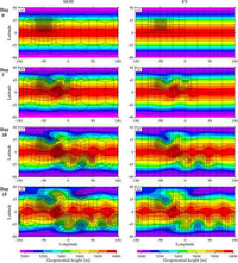
Fig. 8: Snapshots of the geopotential height field (test case 5, flow over a mountain) with three refinement levels at day 0, 5, 10 and 15. The finest grid spacing is $0.625^{\circ}\times 0.625^{\circ}$, the adapted spectral elements (SEM) and blocks (FV) are overlaid. Left column (a-d) shows the SEM model, right column (e-h) depicts the FV model. The refinement criterion is $|\zeta|\geq 2\times 10^{-5}$ s^-1. The contour interval is $100$ m.

The results can be quantitatively compared via normalized error norms which are shown in Fig. 9. An analytic solution is not known. Therefore, the normalized error metrics are computed by comparing the SEM and FV simulations to a T$213$ spectral transform reference solution provided by the National Center for Atmospheric Research (NCAR) (jakob:93, ; jakob:95, ). The latter is available as an archived netCDF data set with daily snapshots of the spectral transform simulation. The T$213$ spectral simulation utilized a Gaussian grid with $320\times 640$ grid points in latitudinal and longitudinal direction which corresponds to a grid spacing of about 55 km at the equator. Figure 9 compares the normalized $l_{2}$ height errors of the adaptive runs to uniform-resolution simulations. Both models are depicted. It is interesting to note that the errors in SEM (Fig. 9a) already converge within the uncertainty of the NCAR reference solution (see Taylor:1997vn ) at the uniform resolution $2.5^{\circ}\times 2.5^{\circ}$. The SEM adaptive run matches this error trace very closely. On the other hand, the errors in FV (Fig. 9 b) converge within the uncertainty of the reference solution at the finer uniform resolution $0.625^{\circ}\times 0.625^{\circ}$. Here, the error trace of the FV adaptive simulation resembles the $2.5^{\circ}\times 2.5^{\circ}$ uniform run despite the higher resolution in the refined areas. It indicates that the coarser domains in FV still contribute considerably to the global $l_{2}$ error measure. In addition, the interpolations in the ghost cell regions add to the error norms.

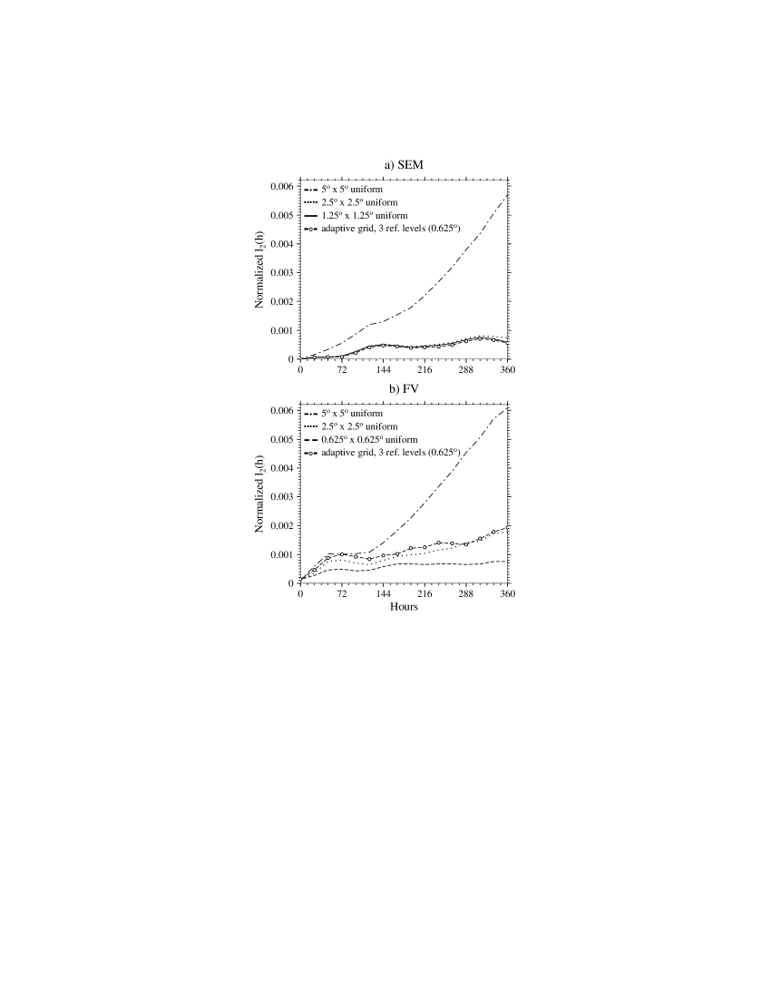
Fig. 9: Time traces of the normalized $l_{2}$ geopotential height error norms for the flow over a mountain (test case 5). The adaptive simulations with three refinement levels ($0.625^{\circ}\times 0.625^{\circ}$ at the finest level) is compared to uniform resolution runs.

4.4 Rossby-Haurwitz wave

The initial condition for test case 6 of the Williamson:1992ts test suite is a wavenumber 4 Rossby-Haurwitz wave. These waves are analytic solutions to the nonlinear non-divergent barotropic vorticity equation, but not closed-form solutions of the barotropic shallow water equations. However, in a shallow water system the wave pattern moves from west to east without change of shape during the course of the integration. The initial conditions are fully described in Williamson:1992ts , the orography field is set to zero. The Rossby-Haurwitz wave with wavenumber 4 exhibits extremely strong gradients in both the geopotential and the wind fields. This test is especially hard for the FV adaptive grid simulations due not only to the strong gradients but also to the dominant $45^{\circ}$ transport angle of the flow in midlatitudes. This challenges the underlying operator splitting approach in FV and accentuates even minor errors.

Both shallow water models are integrated for 14 days on a $2.5^{\circ}\times 2.5^{\circ}$ base grid. This base resolution is identical to test case 2. In addition, static refinements at refinement level 1 $(1.25^{\circ}\times 1.25^{\circ})$ are placed within eight pre-determined regions of interest. In particular, the grid is refined where the initial meridional wind field is $v\leq-60$ m s^-1 which leads to an almost identical number of refined elements and blocks in the two models (Table 2). This rather arbitrary refinement criterion is intended to test whether the wavenumber 4 pattern moves smoothly through the refined grid patches. As an aside, minor improvements of the error norms are expected. The daily simulation results of SEM and FV are compared to the NCAR reference solution (jakob:93, ; jakob:95, ). As for test case 5 (flow over the mountain), the latter is available as an archived netCDF data set that contains the daily results of an NCAR spectral shallow water model at the resolution T$213$ ($\approx$ 55 km).

Figures 10a-b show the geopotential height field of the adaptive SEM and FV model runs at day 7. It can clearly be seen that both SEM and FV maintain the wavenumber 4 pattern of the height field rather well while moving through the refined patches. Here, the results can be visually compared to the NCAR reference solution (Fig. 10c). No noise or distortions are visible at this stage. However, FV develops slight asymmetries in the height field at later times. They originate at the interfaces of the refined areas and slightly disturb the wave field over the course of the integration. These perturbations can again be traced back to ghost cell interpolations in the FV model that now lead to a slight increase in the $l_{2}$ errors norm. The effect is amplified by the very strong gradients in the flow field and the dominant $45^{\circ}$ transport angle. The time steps for these simulations are $15$ s and $225$ s for SEM and FV, respectively.

The error norms for both models are quantitatively compared in Fig. 11. The figure shows the time evolution of the normalized $l_{2}$ height error norms in comparison to fixed-resolution SEM and FV model runs. In particular, two different base resolutions are shown for SEM. These are the regular $2.5^{\circ}\times 2.5^{\circ}$ base grid (216 elements) and a coarser $3.2^{\circ}\times 3.2^{\circ}$ base mesh (96 elements). In both SEM cases, $6\times 6$ GL quadrature points per spectral element are used. The coarser simulation is added since SEM already converges within the uncertainty of the reference solution (Taylor:1997vn, ) on the $2.5^{\circ}$ base grid. Figure 11 shows that SEM exhibits smaller errors than FV at the same uniform resolution. At day 12, the errors in the FV run are rather similar to the coarser $3.2^{\circ}$ SEM simulation. With respect to the static adaptations, SEM does not show an increase in the error in comparison to FV. Instead, the SEM errors in the statically adaptive runs are almost identical to the uniform-mesh simulation or slightly diminish at the end of the forecast period.

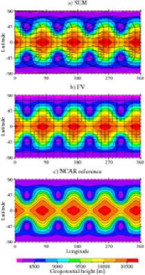
Fig. 10: Snapshots of the geopotential height field of the Rossby-Haurwitz wave (test case 6) at day 7 for (a) SEM, (b) FV and (c) the NCAR spectral model (reference solution). SEM and FV utilize an adaptive grid with one level of static adaptations. The base resolution is $2.5^{\circ}\times 2.5^{\circ}$ and $1.25^{\circ}\times 1.25^{\circ}$ within the refined region. The adapted elements (SEM) and blocks (FV) are overlaid. The contour interval is $250$ m.

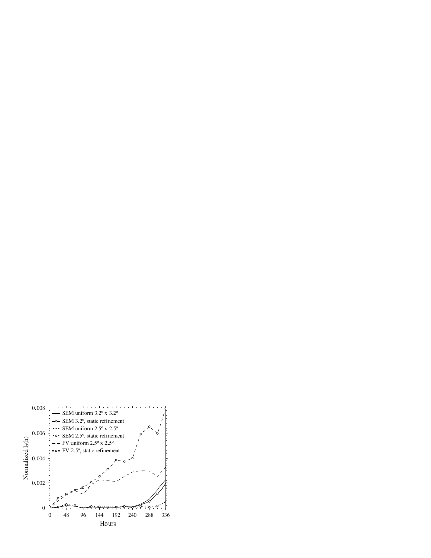
Fig. 11: Time traces of the normalized $l_{2}$ geopotential height error norms for the Rossby-Haurwitz wave (test case 6). The statically adaptive simulations with one refinement levels ($1.25^{\circ}\times 1.25^{\circ}$ at the finest level) are compared to SEM and FV uniform resolution runs.

5 Conclusions

In this paper, two shallow water models with adaptive mesh refinement capabilities are compared. The models are an interpolation-based spectral element model (SEM) on a cubed-sphere grid and a conservative and monotonic finite volume model (FV) in latitude-longitude geometry. Both adaptive mesh approaches utilize a quad-tree AMR technique that reduces the mesh spacings by a factor of two during each refinement step. Coarsenings reverse this adaptations principle. Then four “children/leaves” are coalesced which doubles the grid distances. In SEM, the refinement strategy targets the spectral elements which contain additional Gauss-Legendre and Gauss-Lobatto-Legendre collocation points for scalar and vector components. In FV, the adaptations are applied to a block-data structure in spherical coordinates which consists of a fixed (self-similar) block size. These blocks are surrounded by ghost cell regions which require interpolation and averaging procedures at fine-coarse mesh interfaces. No ghost cells areas are needed in SEM. In both models neighboring elements or blocks can only differ by one refinement level. This leads to cascading and non-conforming refinement regions around the finest mesh.

The models are compared via selected test cases from the standard Williamson:1992ts shallow water test suite. They include the advection of a cosine bell (test 1), a steady-state geostrophic flow (test 2), a flow over a mountain (test 5) and a Rossby-Haurwitz wave (test 6). Both static and dynamics adaptations are assessed which reveal the strengths and weaknesses of the AMR approaches. The AMR simulations show that both models successfully place static and dynamic adaptations in local regions without requiring a fine grid in the global domain. The adaptive grids reliably track the user-selected features of interests without visible distortions or noise at the mesh interfaces. In particular, two dynamic refinement criteria were evaluated. Among them were a simple geopotential height threshold (test 1) as well as the magnitude of the relative vorticity (test 5). The latter successfully steered the SEM and FV refined grids into the Southern Hemisphere at the end of the 15-day forecast period. In addition, two static AMR configurations in user-determined regions of interest were tested. They confirmed that the flows move smoothly through the refined areas in both SEM and FV. Nevertheless, the FV simulations showed that small errors originate at fine-coarse grid interfaces. These errors were due to the interpolation and averaging mechanisms in the ghost cell regions of the block-data structure. This was not the case in SEM which exhibited a decrease in error whenever adaptations were introduced.

Overall, the number of dynamically refined elements or blocks was comparable in both models if the adaptations were confined to the equatorial or midlatitudinal regions. In polar regions though, the number of refined blocks in FV exceeded the number of refined elements in SEM considerably due to the convergence of the meridians in the latitude-longitude grid. In general, it was shown that SEM exhibited smaller errors than FV for all test cases at identical resolutions. This is expected for SEM’s high-order numerical technique despite its non-conservative and non-monotonic nature. The latter can cause spurious oscillations and negative values for positive-definite fields (test 1). In contrast, the FV technique is mass-conservative and monotonic which, on the other hand, introduces numerical dissipation through its monotonicity constraint. The dissipation is reduced at high resolutions. Then the SEM and FV simulations resemble each other very closely.

The problem of conservation and the removal of some of the oscillations in SEM can be addressed by using the discontinuous Galerkin (DG) formulation. Future developments will include an evaluation of the DG method as well as efficient time-stepping techniques (Nair:2005aj, ; St-Cyr:2005jw, ; St-Cyr:2005ur, ; St-Cyr:2006xf, ) to avoid the very small time steps for numerical stability. In addition, tests involving strong jets such as in Galewsky:2004wa and laeuter:05 , effects of orography and a full GCM comparison will be the subject of interesting future research.

References

- (1) Bacon, D. P., Ahmad, N. N., Boybeyi, Z., Dunn, T. J., Hall, M. S., Lee, P. C. S., Sarma, R. A., Turner, M. D., III, K. T. W., Young, S. H., and Zack, J. W. A dynamically adapting weather and dispersion model: The operational multiscale environment model with grid adaptivity (OMEGA). Mon.Wea. Rev. 128 (2000), 2044–2076.
- (2) Behrens, J. Adaptive Atmospheric Modeling - Key techniques in grid generation, data structures, and numerical operations with applications. Springer, 2006. Lecture Notes in Computational Science and Engineering, ISBN 3-540-33382-7, 207 pp.
- (3) Behrens, J., Rakowsky, N., Hiller, W., Handorf, D., Läuter, M., Päpke, J., and Dethloff, K. amatos: Parallel adaptive mesh generator for atmospheric and oceanic simulation. Ocean Modelling 10 (2005), 171–183.
- (4) Boyd, J. P. The Erfc-Log filter and the asymptotics of the Euler and Vandeven sequence accelerations. In Proceedings of the Third International Conference on Spectral and High Order Methods (1996), A. V. Ilin and L. R. Scott, Eds., Third International Conference on Spectral and High Order Methods, Houston Journal of Mathematics, pp. 267–276.
- (5) Boyd, J. P. Book review: High-order methods for incompressible fluid flow. . SIAM Rev. 46, 1 (2004), 151–157.
- (6) Carpenter, R. L., Droegemeier, K. K., Woodward, P. R., and Hane, C. E. Application of the Piecewise Parabolic Method (PPM) to meteorological modeling. Mon. Wea. Rev. 118 (March 1990), 586–612.
- (7) Colella, P., and Woodward, P. R. The piecewise parabolic method (PPM) for gas-dynamical simulations. J. of Comput. Phys. 54 (1984), 174–201.
- (8) Dennis, J. M. Partitioning with space-filling curves on the cubed sphere. In Proc. International Parallel and Distributed Processing Symposium (IPDPS) (Nice, France, April 2003), IEEE/ACM. CD-ROM. No. 269a.
- (9) Deville, M. O., Fischer, P. F., and Mund, E. H. High-Order Methods for Incompressible Fluid Flow. Cambridge monographs on applied and computational mathematics. Cambridge University Press, 2002.
- (10) Dietachmayer, G. S., and Droegemeier, K. K. Application of continuous dynamic grid adaptation techniques to meteorological modeling. part i: Basic formulation and accuracy. Mon. Wea. Rev. 120 (1992), 1675–1706.
- (11) Feng, H., and Mavriplis, C. Adaptive Spectral Element Simulations of Thin Flame Sheet Deformations. J. Sci. Comput. 17 (2002), 1–3.
- (12) Fischer, P. F., Kruse, G., and Loth, F. Spectral element methods for transitional flows in complex geometries. J. Sci. Comput. 17 (2002), 81–98.
- (13) Fournier, A., Taylor, M. A., and Tribbia, J. J. The spectral element atmosphere model (SEAM): High-resolution parallel computation and localized resolution of regional dynamics. Mon. Wea. Rev. 132, 3 (2004), 726–748.
- (14) Frohn, L. M., Christensen, J. H., and Brandt, J. Development of a high-resolution nested air pollution model – the numerical approach. J. Comput. Phys. 179 (2002), 68–94.
- (15) Galewsky, J., Scott, R. K., and Polvani, L. M. An initial-value problem for testing numerical models of the global shallow water equations. Tellus, A 56, 5 (2004), 429–440.
- (16) Gibbs, J. W. Fourier Series. Nature 59 (1899), 606.
- (17) Giraldo, F. X. The Lagrange-Galerkin method for the two-dimensional shallow water equations on adaptive grids. Int. J. Numer. Meth. Fluids 33 (2000), 789–832.
- (18) Giraldo, F. X. A spectral element shallow water model on spherical geodesic grids. Int. J. Numer. Meth. Fluids 35 (2001), 869–901.
- (19) Giraldo, F. X. High-order triangle-based discontinuous Galerkin methods for hyperbolic equations on a rotating sphere. J. Comput. Phys 214 (2006), 447–465.
- (20) Giraldo, F. X., and Warburton, T. A nodal triangle-based spectral element method for the shallow water equations on the sphere. J. Comput. Phys. 207, 1 (2005), 129–150.
- (21) Gopalakrishnan, S. G., Bacon, D. P., Ahmad, N. N., Boybeyi, Z., Dunn, T. J., Hall, M. S., Jin, Y., Lee, P. C. S., Mays, D. E., Madala, R. V., Sarma, A., Turner, M. D., and Wait, T. R. An operational multiscale hurricane forecasting system. Mon. Wea. Rev. 130 (2002), 1830–1847.
- (22) Haidvogel, D., Curchitser, E., Iskandarani, M., Hughes, R., and Taylor, M. Global modeling of the ocean and atmosphere using the spectral element method. Atmos.-Ocean 35 (1997), 505.
- (23) Iselin, J., Gutowski, W. J., and Prusa, J. M. Tracer advection using dynamic grid adaptation and MM5. Mon. Wea. Rev. 133 (2005), 175–187.
- (24) Iselin, J., Prusa, J. M., and Gutowski, W. J. Dynamic grid adaptation using the MPDATA scheme. Mon. Wea. Rev. 130 (2002), 1026–1039.
- (25) Jablonowski, C. Adaptive Grids in Weather and Climate Modeling. PhD thesis, University of Michigan, Ann Arbor, MI, 2004. Department of Atmospheric, Oceanic and Space Sciences, 292 pp.
- (26) Jablonowski, C., Herzog, M., Penner, J. E., Oehmke, R. C., Stout, Q. F., and van Leer, B. Adaptive grids for weather and climate models. In ECMWF Seminar Proceedings on Recent Developments in Numerical Methods for Atmosphere and Ocean Modeling (Reading, United Kingdom, September 2004), ECMWF, pp. 233–250.
- (27) Jablonowski, C., Herzog, M., Penner, J. E., Oehmke, R. C., Stout, Q. F., and van Leer, B. Adaptive grids for atmospheric general circulation models: Test of the dynamical core, 2006. to be submitted to Mon. Wea. Rev.
- (28) Jablonowski, C., Herzog, M., Penner, J. E., Oehmke, R. C., Stout, Q. F., van Leer, B., and Powell, K. G. Block-structured adaptive grids on the sphere: Advection experiments. Mon. Wea. Rev. 134, 12 (2006), 3691–3713.
- (29) Jakob, R., Hack, J. J., and Williamson, D. L. Solutions to the shallow-water test set using the spectral transform method. Tech. Rep. NCAR/TN-388+STR, National Center for Atmospheric Research, Boulder, Colorado, 1993.
- (30) Jakob-Chien, R., Hack, J. J., and Williamson, D. L. Spectral transform solutions to the shallow water test set. Journal of Computational Physics 119 (1995), 164–187.
- (31) Karypis, G., Schloegel, K., and Kumar, V. ParMetis: Parallel Graph Partitioning and Sparse Matrix Ordering Library, Version 3.0. University of Minnesota, 2002.
- (32) Kurihara, Y., and Bender, M. A. Use of a movable nested-mesh model for tracking a small vortex. Mon. Wea. Rev. 108 (1980), 1792–1809.
- (33) Kurihara, Y., Tripoli, G. J., and Bender, M. A. Design of a movable nested-mesh primitive equation model. Mon. Wea. Rev. 107 (1979), 239–249.
- (34) Läuter, M. Großräumige Zirkulationsstrukturen in einem nichtlinearen adaptiven Atmosphärenmodell. PhD thesis, Universität Potsdam, Germany, 2004. Wissenschaftsdisziplin Physik der Atmophäre, 135 pp.
- (35) Läuter, M., Handorf, D., and Dethloff, K. Unsteady analytical solutions of the spherical shallow water equations. J. Comput. Phys. 210 (2005), 535–553.
- (36) Läuter, M., Handorf, D., Rakowsky, N., Behrens, J., Frickenhaus, S., Best, M., Dethloff, K., and Hiller, W. A parallel adaptive barotropic model of the atmosphere, 2006. J. Comput. Phys., accepted.
- (37) Lin, S.-J., and Rood, R. B. Multidimensional flux-form semi-Lagrangian transport scheme. Mon. Wea. Rev. 124 (September 1996), 2046–2070.
- (38) Lin, S.-J., and Rood, R. B. An explicit flux-form semi-Lagrangian shallow water model on the sphere. Quart. J. Roy. Meteor. Soc. 123 (1997), 2477–2498.
- (39) Mavriplis, C. Nonconforming Discretizations and a Posteriori Error Estimators for Adaptive Spectral Element Techniques. PhD thesis, MIT, Boston, MA., 1989. 156 pp.
- (40) Nair, R. D., and Machenhauer, B. The mass-conservative cell-integrated semi-Lagrangian advection scheme on the sphere. Mon. Wea. Rev. 130 (March 2002), 649–667.
- (41) Nair, R. D., Thomas, S. J., and Loft, R. D. A discontinuous Galerkin global shallow water model. Mon. Wea. Rev. 133, 4 (2005), 876–888.
- (42) Oehmke, R. C. High Performance Dynamic Array Structures. PhD thesis, University of Michigan, Ann Arbor, MI, USA, 2004. 93 pp.
- (43) Oehmke, R. C., and Stout, Q. F. Parallel adaptive blocks on a sphere. In Proc. 10th SIAM Conference on Parallel Processing for Scientific Computing (Portsmouth, Virginia, USA, 2001), SIAM. CD-ROM.
- (44) Patera, A. T. A spectral element method for fluid dynamics: Laminar flow in a channel expansion. J. Comput. Phys. 54 (1984), 468–488.
- (45) Prusa, J. M., and Smolarkiewicz, P. K. An all-scale anelastic model for geophysical flows: dynamic grid deformation. J. Comput. Phys. 190 (2003), 601–622.
- (46) Quarteroni, A., and Valli, A. Numerical Approximations of Partial Differential Equations, vol. 23 of Springer series in computational mathematics. Springer-Verlag, 1997.
- (47) Rosenberg, D., Fournier, A., Fischer, P., and Pouquet, A. Geophysical–astrophysical spectral-element adaptive refinement (GASpAR): Object-oriented h-adaptive fluid dynamics simulation. J. Comput. Phys. 215 (2006), 59–80.
- (48) Sadourny, R. Conservative finite-difference approximations of the primitive equations on quasi-uniform spherical grids. Mon. Wea. Rev. 100 (1972), 136–144.
- (49) Skamarock, W. C. Truncation error estimates for refinement criteria in nested and adaptive models. Mon. Wea. Rev. 117 (1989), 872–886.
- (50) Skamarock, W. C., and Klemp, J. B. Adaptive grid refinement for twodimensional and three-dimensional nonhydrostatic atmospheric flow. Mon. Wea. Rev. 121 (1993), 788–804.
- (51) Skamarock, W. C., Oliger, J., and Street, R. L. Adaptive grid refinement for numerical weather prediction. J. Comput. Phys. 80 (1989), 27–60.
- (52) Smolarkiewicz, P. K. Multidimensional positive definite advection transport algorithm: an overview. Int. J. Num. Meth. Fluids 50, 10 (2006), 1123–1144.
- (53) Smolarkiewicz, P. K., and Szmelter, J. MPDATA: an edge-based unstructured-grid formulation. J. Comput. Phys. 206, 2 (2005), 624–649.
- (54) St-Cyr, A., Dennis, J. M., Thomas, S. J., and Tufo, H. M. Operator splitting in a non-conforming adaptive spectral element atmospheric model. SIAM J. Sci. Comput., submitted, 2006.
- (55) St-Cyr, A., and Thomas, S. J. Nonlinear OIFS for a hybrid Galerkin atmospheric model. In Lecture notes in computer science (2005), vol. LNCS 3516 of Lecture Notes in Computer Science, pp. 57–63.
- (56) St-Cyr, A., and Thomas, S. J. Nonlinear operator-integration factor splitting for the shallow water equations. Appl. Numer. Math. 52 (2005), 429–448.
- (57) Taylor, M., Tribbia, J., and Iskandarani, M. The spectral element method for the shallow water equations on the sphere. J. Comput. Phys. 130, 1 (1997), 92–108.
- (58) Thomas, S. J., and Loft, R. D. Semi-implicit spectral element atmospheric model. J. Sci. Comp. 17 (2002), 339–350.
- (59) Tolstykh, M. A. Vorticity-divergence semi-Lagrangian shallow-water model of the sphere based on compact finite differences. J. Comput. Phys. 179 (2002), 180–200.
- (60) Tufo, H. M. Algorithms for large-scale parallel simulations of unsteady incompressible flows in three-dimensional complex geometries. PhD thesis, Division of Applied Mathematics, Brown University, Providence, R.I., 1998.
- (61) Vandeven, H. Family of spectral filters for discontinuous problems. J. Sci. Comput. 6 (1991), 159–192.
- (62) Wilhelm, D., and Kleiser, L. Stable and unstable formulation of the convection operator in spectral element simulations. Appl. Numer. Math. 33 (2000), 275–280.
- (63) Williamson, D. L., Drake, J. B., Hack, J. J., Jakob, R., and Swarztrauber, P. N. A standard test set for numerical approximations to the shallow water equations in spherical geometry. J. Comp. Phys. 102 (1992), 211–224.