Classical light dispersion theory in a regular lattice

Abstract

We study the dynamics of an infinite regular lattice of classical charged oscillators. Each individual oscillator is described as a point particle subject to a harmonic restoring potential, to the retarded electromagnetic field generated by all the other particles, and to the radiation reaction expressed according to the Lorentz–Dirac equation. Exact normal mode solutions, describing the propagation of plane electromagnetic waves through the lattice, are obtained for the complete linearized system of infinitely many oscillators. At variance with all the available results, our method is valid for any values of the frequency, or of the ratio between wavelength and lattice parameter. A remarkable feature is that the proper inclusion of radiation reaction in the dynamics of the individual oscillators does not give rise to any extinction coefficient for the global normal modes of the lattice. The dispersion relations resulting from our solution are numerically studied for the case of a simple cubic lattice. New predictions are obtained in this way about the behavior of the crystal at frequencies near the proper oscillation frequency of the dipoles.

I Introduction

The classical theory of dispersion is a subject with a long and noble history born1 ; BW . Although the main features of the phenomenon can be described by treating matter as a continuum characterized by macroscopic quantities such as the electric and magnetic polarizations, it is clear that a truly fundamental theory has to be based on a microscopic model of matter. We shall now try to summarize some crucial aspects of the problem in an historical perspective, before illustrating the new features of our present approach.

By treating an elementary electric dipole as an oscillator subject to a linear restoring force, it is possible to obtain a simple expression for the molecular polarizability, i.e. the complex frequency-dependent linear coefficient which relates the microscopic dipole moment to the amplitude of the incident electromagnetic radiation. In order to correctly apply this simple model to the description of the behavior of a large system of mutually interacting dipoles, one has however to consider that the field acting on each microscopic oscillator cannot be simply identified with the macroscopic electromagnetic field in the medium. In fact, while the latter simply represents the average of the microscopic field over a region much larger than the intermolecular spacing, the former has to be carefully calculated by evaluating and summing, on the site occupied by the considered dipole, the retarded fields generated by all the other dipoles of the medium. This “exciting” field (as we shall refer to in the following, although the names “effective” or “local” field have also been employed in the literature) was theoretically estimated by Lorentz already at the end of nineteenth century lorentz1 ; lorentz2 ; lorentz3 ; lorentz4 by dividing the medium into two regions separated by a virtual sphere surrounding the considered dipole. He restricted his attention to the typical situation in which the wavelength of the macroscopic electromagnetic field is of a larger order of magnitude than the average intermolecular spacing, so that one can take for the virtual sphere a radius intermediate between the two. He then argued that the influence of the portion of the medium lying outside the sphere can be fairly approximated as that of a continuous distribution of electric dipole moment, whereas the sum of the forces exerted by all the dipoles situated inside the sphere can be assumed to vanish in most cases on the basis of symmetry considerations. A rather similar analysis, leading to equivalent conclusions, was also carried out by Planck planck . With these arguments one can derive the well-known Lorentz–Lorenz formula lorentz2 ; lorenz , relating the macroscopic dielectric constant of the medium to the molecular polarizability, and it is thus possible to deduce an approximate expression for the dispersion relation of an array of oscillators in the long-wavelength regime (which generally includes the optical frequencies).

A detailed microscopic theory of dispersion in a crystalline solid, although with neglect of radiation reaction, was formulated by Ewald ewald2 ; ewald1 . He considered a rectangular parallelepiped as the unit cell of the Bravais lattice, and his results were subsequently generalized by Born to more general crystal structures born2 ; born1 . The mathematical methods used by these authors (one has to keep in mind that the theory of distributions was not yet existing at that time) led however to rather clumsy expressions for the exciting field, which could be numerically evaluated only in the limit of an infinitely large ratio between wavelength and lattice constant, i.e. still essentially in the continuum approximation. In this way the previous results by Lorentz and Planck were recovered for structures with tetrahedral symmetry. Furthermore, in the case of parallelepipeds of unequal edges, Ewald was able to perform in the same limit a numerical calculation relating the ratio between the edges to the phenomenon of double refraction. Finally, Ewald extended his analysis of the model also to the study of X-ray diffraction ewald3 , but he made use to this purpose of other important simplifications which are possible only in the opposite limit of a radiation frequency much higher that the characteristic frequencies of the crystal.

Many investigations were later devoted to the application of quantum mechanics to the theory of light dispersion, and the results of Ewald and Born were apparently considered to be the final word about the problem of the mutual interaction of a large array of classical resonators. We are going to prove that, on the contrary, a deeper analysis reveals important properties of this fundamental dynamical system which have been for many decades completely overlooked.

In the present paper we shall study a system of infinitely many charged particles, subject to linear restoring forces towards their equilibrium positions at the sites of a regular lattice, and interacting with each other through the retarded electromagnetic fields. Our outset will therefore be similar to Ewalds’s, but with inclusion in the equations of motion of the usual “triple-dot” radiation reaction term, which corresponds to the nonrelativistic form of the Lorentz–Dirac equation lorentz4 ; dirac . The only approximation that we shall use is that of small oscillations: this will allow us still to deal with a system of linear equations. We shall provide a general and rigorous procedure for the calculation of the exciting field, avoiding to introduce at any stage of the procedure the continuum approximation. This will be accomplished by a method involving the careful subtraction of two divergent quantities (representing respectively the total field and the field generated by the dipole under consideration), which appears to be more powerful than that used by Ewald and Born, and presents some formal analogy with the renormalization techniques of quantum field theory. Using our procedure we shall show that for an infinite regular lattice there exists a continuous set of normal modes which describe the propagation of plane electromagnetic waves.

A remarkable result will be that the inclusion of the radiation damping term in the equations of motion of the oscillating particles, instead of giving rise to an extinction coefficient for the wave, as is commonly believed according to the standard approximated treatments of the model, is on the contrary essential for justifying the presence of undamped collective waves. Such a result in fact constitutes an extension to the three dimensional case of an analogous one already obtained by two of the present authors for the case of a rectilinear chain of one-dimensional oscillators CG . It relies upon a remarkable identity which was originally formulated in a different context by Wheeler and Feynman WF . These authors deduced it from the hypothesis of the “complete absorber”, which they introduced in order make their time-reversible action-at-a-distance electrodynamics compatible with the observed phenomenon of radiation reaction. For the physical system here considered we are going to prove in a simple and direct way that, although no absorption mechanism is present in the model, this “Wheeler–Feynman identity” actually holds as a purely mathematical property of the entire class of solutions on which we are interested.

By numerically studying the dispersion relations for the crystal, as resulting from the exact solutions of the model, it will also be shown that completely new features appear for frequencies in a region about the proper frequency of the oscillators. In such a region the wavelength can in fact become as short as the lattice spacing, so that the approximations adopted in the previous literature become unavailable, and only an exact solution can give predictions about the behavior of the system. It is found that inside the interval of frequencies where undamped wave propagation was believed to be impossible, plane waves can actually propagate, with very low group velocities, along certain lattice directions and for appropriate wave polarization.

II The model

Let us consider an infinite three-dimensional simple Bravais lattice, that is an array of points

$${\bf r}_{{\bf n}}=n_{1}{\bf a}_{1}+n_{2}{\bf a}_{2}+n_{3}{\bf a}_{3}\,,$$ (1)

where ${\bf n}$ denotes the triple of relative integers $(n_{1},n_{2},n_{3})$, and ${\bf a}_{1}$, ${\bf a}_{2}$, ${\bf a}_{3}$ are a set of primitive translation vectors for the lattice kittel . We choose the orientation of the ${\bf a}_{i}$ in such a way that $V={\bf a}_{1}\cdot{\bf a}_{2}\times{\bf a}_{3}>0$. $V$ clearly represents the volume of the primitive cell. Each point ${\bf r}_{{\bf n}}$ is the equilibrium position of a point particle (electron) of mass $m$ and electric charge $e$, which is subject to an elastic force of the form

$${\bf F}_{{\rm el}}=-K({\bf z}_{{\bf n}}-{\bf r}_{{\bf n}})\,,$$

where the vector ${\bf z}_{{\bf n}}$ represents the instantaneous coordinates of the point particle. Although it is not strictly necessary for the mathematical self-consistency of the model, in order to reproduce in a more realistic way the situation of solid state physics we can assume that ${\bf r}_{{\bf n}}$ is also the seat of a static positive ion of charge $-e$. As is traditionally the case for the classical models of dispersion, we shall neglect the Coulomb interaction between the ion and its associated electron, since classical mechanics fails at such short distance scales, and we shall instead identify the proper oscillator frequency $\omega_{0}=\sqrt{K/m}$ with a characteristic excitation frequency of the optical electron in the atomic ground state. According to quantum mechanics, it could even be possible to obtain a more realistic model by associating to each atom a set of fictitious oscillators becker , one for each allowed quantum transition from the ground state of energy $E_{0}$ to an excited state of energy $E_{n}$, with proper frequencies $\omega_{0n}=(E_{n}-E_{0})/\hbar$. In order to assign to the contribution of each oscillator an appropriate weight, one has then to make the substitution $e^{2}/m\rightarrow f_{0n}e^{2}/m$, where the “oscillator strengths” $f_{0n}$ are coefficients subject to the sum rule $\sum_{n}f_{0n}=1$ (we are considering here atoms with a single optically active electron). An explicit calculation from first order perturbation theory provides

$$f_{0n}=(2m/\hbar)\omega_{0n}\left|\left\langle E_{0}\left|\bm{\varepsilon}\cdot{\bf\hat{x}}\right|E_{n}\right\rangle\right|^{2},$$

${\bf\hat{x}}$ being the position operator and $\bm{\varepsilon}$ the unit vector representing the direction of oscillation. For the sake of simplicity we shall consider in the following calculations a single oscillator per atom, in accordance with the original literature on classical dispersion, although the extension to the case of multiple oscillators presents no conceptual difficulty.

The charge and current densities associated with the electron-ion pair are given respectively by

$$\rho_{{\bf n}}({\bf x},t) = e\left[\delta^{3}({\bf x}-{\bf z}_{{\bf n}}(t))-\delta^{3}({\bf x}-{\bf r}_{{\bf n}})\right]$$ (2)

$${\bf j}_{{\bf n}}({\bf x},t) = e{\bf\dot{z}}_{{\bf n}}(t)\delta^{3}({\bf x}-{\bf z}_{{\bf n}}(t))\,,$$ (3)

where $\delta$ denotes Dirac’s delta function. The retarded potentials generated by the charge-current density $j_{{\bf n}}^{\mu}$ (with $j^{0}_{\bf n}\equiv c\rho_{\bf n}$) are defined as

$$A_{{\bf n}}^{\mu,{\rm ret}}(x) = \frac{1}{c}\int d^{4}y\,D_{{\rm ret}}(x-y)j_{{\bf n}}^{\mu}(y)$$ (4)

$$= \frac{1}{(2\pi)^{4}c}\int d^{4}k\,\frac{e^{ik\cdot x}}{k^{2}-i\varepsilon k^{0}}\tilde{j}_{{\bf n}}^{\mu}(k)\,,$$

where

$$\,D_{{\rm ret}}(x)=\frac{\delta(x^{0}-\left|{\bf x}\right|)}{4\pi\left|{\bf x}\right|}=\frac{1}{(2\pi)^{4}}\int d^{4}k\,\frac{e^{ik\cdot x}}{k^{2}-i\varepsilon k^{0}}$$ (5)

is the retarded Green function jackson and

$$\tilde{j}_{{\bf n}}^{\mu}(k)=\int d^{4}y\,e^{-ik\cdot y}j_{{\bf n}}^{\mu}(y)$$ (6)

is the Fourier transform of $j_{{\bf n}}^{\mu}$. We are here using the four-dimensional notation so that, for instance, $x$ denotes the four-vector $(x^{0},{\bf x})$, and $x^{0}=ct$, $k\cdot x=k_{\mu}x^{\mu}={\bf k}\cdot{\bf x}-k^{0}x^{0}$, $k^{2}=k\cdot k={\bf k}^{2}-(k^{0})^{2}$. Summation over repeated indices is always implicitly understood. The retarded potentials satisfy the equation

$$\partial^{\nu}\partial_{\nu}A_{{\bf n}}^{\mu,{\rm ret}}=-\frac{1}{c}j_{{\bf n}}^{\mu}$$

and the Lorentz gauge condition

$$\partial_{\mu}A_{{\bf n}}^{\mu,{\rm ret}}=0\,.$$

Introducing then the retarded fields according to the usual relations

$${\bf E}_{\bf n}^{\rm ret} = -{\bf\nabla}A_{\bf n}^{0,{\rm ret}}-\frac{\partial}{c\partial t}{\bf A}_{\bf n}^{\rm ret}$$ (7)

$${\bf B}_{\bf n}^{\rm ret} = {\bf\nabla}\times{\bf A}_{\bf n}^{\rm ret}$$ (8)

and putting ${\bf x}_{{\bf n}}={\bf z}_{{\bf n}}-{\bf r}_{{\bf n}}$, we can write the (nonrelativistic) equation of motion of the electrons as

$$m{\bf\ddot{x}}_{{\bf n}} = -K{\bf x}_{{\bf n}}+e{\bf e}_{{\bf n}}({\bf r}_{{\bf n}}+{\bf x}_{{\bf n}},t)$$ (9)

$$+e{\bf\dot{x}}_{{\bf n}}\times{\bf b}_{{\bf n}}({\bf r}_{{\bf n}}+{\bf x}_{{\bf n}},t)+\frac{e^{2}}{6\pi c^{3}}\dddot{\bf x}_{{\bf n}}\,,$$

where

$${\bf e}_{{\bf n}} = \sum_{{\bf m}\neq{\bf 0}}{\bf E}_{{\bf n}+{\bf m}}^{\rm ret}$$ (10)

$${\bf b}_{{\bf n}} = \sum_{{\bf m}\neq{\bf 0}}{\bf B}_{{\bf n}+{\bf m}}^{\rm ret}$$ (11)

represent the exciting fields. The notation used in the two last equations means that the summation index $\bf m$ runs over all the values in $\mathbb{Z}^{3}$ except $\bf 0$. The last term in Eq. (9) describes the radiation reaction force, according to the Lorentz–Dirac prescription. See Ref. milonni for a comparison between the expression of the atomic polarizability resulting from this classical equation in the dipole approximation, and the corresponding result obtained for a two-level atom in electric-dipole interaction with the quantized electromagnetic field.

III Normal-mode solutions

We suppose the amplitude of the oscillations to be small enough, so that at every stage we can neglect all terms of order higher than one in the ${\bf x}_{{\bf n}}$ and their time derivatives of any order. It follows that Eq. (9) simplifies to

$$m{\bf\ddot{x}}_{{\bf n}}=-K{\bf x}_{{\bf n}}+e{\bf e}_{{\bf n}}({\bf r}_{{\bf n}},t)+\frac{e^{2}}{6\pi c^{3}}\dddot{\bf x}_{{\bf n}}\,,$$ (12)

where the retarded fields, included into ${\bf e}_{{\bf n}}$ according to Eq. (10), are to be calculated in the dipole approximation, whereby each ${\bf E}_{\bf m}^{\rm ret}$ depends linearly on ${\bf x}_{{\bf m}}$ and its time derivatives. Of course, Eq. (12) actually represents an infinite system of coupled linear equations, since we have one such equation for each ${\bf n}\in\mathbb{Z}^{3}$. We shall look for a global solution of the form (in customary complex notation)

$${\bf x}_{{\bf n}}={\bf C}\exp\left[i(\bm{\kappa}\cdot{\bf r}_{{\bf n}}-\omega t)\right]\,,$$ (13)

representing a plane wave with amplitude ${\bf C}$, frequency $\omega$ and wavevector $\bm{\kappa}$. The parameters $\omega$ and $\bm{\kappa}$ can always be chosen so that $\omega>0$ and $\bm{\kappa}$ belongs to the first Brillouin zone of the crystal. We shall proceed as follows: for a generic motion of the form (13) we shall calculate the resulting expression for the exciting field ${\bf e}_{{\bf n}}$; then by substituting this expression into Eq. (12) we shall find out that the equations of motion of all the particles can be simultaneously satisfied, provided that $\bm{\kappa}$ and $\omega$ satisfy a well defined dispersion relation.

In the dipole approximation, that is to first order in ${\bf C}$, the charge and current densities become

$$\rho_{{\bf n}}({\bf x},t) = -e{\bf C\cdot\nabla}\delta^{3}({\bf x}-{\bf r}_{{\bf n}})\exp\left[i(\bm{\kappa}\cdot{\bf r}_{{\bf n}}-\omega t)\right]$$

$${\bf j}_{{\bf n}}({\bf x},t) = -ie\omega{\bf C}\delta^{3}({\bf x}-{\bf r}_{{\bf n}})\exp\left[i(\bm{\kappa}\cdot{\bf r}_{{\bf n}}-\omega t)\right]$$

whence, according to the definition (6)

$$\tilde{\rho}_{{\bf n}}(k) = -2\pi ie{\bf k\cdot C}\delta(k^{0}-\omega/c)\exp\left[i(\bm{\kappa}-{\bf k}){\bf\cdot r}_{{\bf n}}\right]$$ (14)

$${\bf\tilde{j}}_{{\bf n}}(k) = -2\pi ie\omega{\bf C}\delta(k^{0}-\omega/c)\exp\left[i(\bm{\kappa}-{\bf k}){\bf\cdot r}_{{\bf n}}\right]\,.$$ (15)

Substituting these expressions into Eq. (4) and then applying Eq. (7) we get

$${\bf E}_{\bf m}^{\rm ret}({\bf x},t) = e\exp\left[i(\bm{\kappa}\cdot{\bf r}_{{\bf m}}-\omega t)\right]$$ (16)

$$\times\int\frac{d^{3}{\bf k}}{(2\pi)^{3}}\,\frac{(\omega/c)^{2}{\bf C}-({\bf k}\cdot{\bf C}){\bf k}}{{\bf k}^{2}-(\omega/c)^{2}-i\varepsilon}$$

$$\times\exp\left[i{\bf k\cdot(x}-{\bf r}_{{\bf m}})\right]\,.$$

It follows

$${\bf e}_{{\bf n}}({\bf r}_{{\bf n}},t)=e{\bf\hat{L}}^{{\rm ret}}(\bm{\kappa},\omega)\cdot{\bf C}\exp\left[i(\bm{\kappa}\cdot{\bf r}_{{\bf n}}-\omega t)\right]\,,$$ (17)

where the second rank tensor ${\bf\hat{L}}^{{\rm ret}}$ has components

$$L^{{\rm ret}}_{ij}(\bm{\kappa},\omega) = \sum_{{\bf m}\neq{\bf 0}}\int\frac{d^{3}{\bf k}}{(2\pi)^{3}}\,\frac{(\omega/c)^{2}\delta_{ij}-k_{i}k_{j}}{{\bf k}^{2}-(\omega/c)^{2}-i\varepsilon}$$

$$\times\exp\left[i({\bf k}-\bm{\kappa})\cdot{\bf r}_{{\bf m}}\right]$$

and we have used the notation ${\bf\hat{L}}^{{\rm ret}}\cdot{\bf C}$ to denote the vector with components $L^{{\rm ret}}_{ij}C_{j}$. By substituting the expressions (13) and (17) into Eq. (12), the original system of infinitely many coupled equations is transformed into the single vectorial equation

$$\frac{e^{2}}{m}{\bf\hat{L}}^{{\rm ret}}(\bm{\kappa},\omega)\cdot{\bf C}=\left(\omega_{0}^{2}-\omega^{2}-i\frac{\omega^{3}e^{2}}{6\pi mc^{3}}\right){\bf C}\,,$$ (18)

which admits solutions with nonvanishing ${\bf C}$ when

$$\det\left[\frac{e^{2}}{m}{\bf\hat{L}}^{{\rm ret}}(\bm{\kappa},\omega)-\left(\omega_{0}^{2}-\omega^{2}-i\frac{\omega^{3}e^{2}}{6\pi mc^{3}}\right){\bf\hat{1}}\right]=0\,.$$ (19)

The above equation determines an implicit relation between $\bm{\kappa}$ and $\omega$, which constitutes the sought for dispersion relation of the crystal.

Once a solution of the form (13) has been obtained, it is easy to write down the expression for the macroscopic quantities which can be associated to the normal mode. The macroscopic polarization density is in fact given by the continuous function of space which interpolates the microscopic displacement vectors of the individual dipoles:

$${\bf P}({\bf x},t)=V^{-1}e{\bf C}\exp\left[i(\bm{\kappa}\cdot{\bf x}-\omega t)\right]\,.$$ (20)

The macroscopic fields ${\bf E}_{\rm mac}$, ${\bf B}_{\rm mac}$ and ${\bf D}_{\rm mac}\equiv{\bf E}_{\rm mac}+{\bf P}$ are then given by the solutions of the usual macroscopic Maxwell equations inside the (nonmagnetic) medium:

$${\bf\nabla}\cdot{\bf D}_{\rm mac} = 0$$ (21)

$${\bf\nabla}\times{\bf E}_{\rm mac} = -\frac{\partial}{c\partial t}{\bf B}_{\rm mac}$$ (22)

$${\bf\nabla}\cdot{\bf B}_{\rm mac} = 0$$ (23)

$${\bf\nabla}\times{\bf B}_{\rm mac} = \frac{\partial}{c\partial t}{\bf D}_{\rm mac}\,.$$ (24)

From Eq. (21) it follows ${\bf\nabla}\cdot{\bf E}_{\rm mac}=-{\bf\nabla}\cdot{\bf P}$. Then by taking the curl of Eq. (22) and eliminating ${\bf B}_{\rm mac}$ with the aid of Eq. (24) one easily obtains

$$\Delta{\bf E}_{\rm mac}-\frac{\partial^{2}}{c^{2}\partial t^{2}}{\bf E}_{\rm mac}=\frac{\partial^{2}}{c^{2}\partial t^{2}}{\bf P}-{\bf\nabla}({\bf\nabla}\cdot{\bf P})\,.$$

From this, Eq. (20) and Eq. (22), we conclude

$${\bf E}_{\rm mac}({\bf x},t) = \frac{e}{V}\frac{(\omega/c)^{2}{\bf C}-\bm{\kappa}(\bm{\kappa}\cdot{\bf C})}{\bm{\kappa}^{2}-(\omega/c)^{2}}$$ (25)

$$\times\exp\left[i(\bm{\kappa}\cdot{\bf x}-\omega t)\right]$$

$${\bf B}_{\rm mac}({\bf x},t) = \frac{e}{V}\frac{(\omega/c)\bm{\kappa}\times{\bf C}}{\bm{\kappa}^{2}-(\omega/c)^{2}}$$ (26)

$$\times\exp\left[i(\bm{\kappa}\cdot{\bf x}-\omega t)\right]\,.$$

IV The Wheeler–Feynman identity

Since (19) is a complex equation, it is a priori to be expected that, in order that a real solution for $\omega$ may exist, the vector $\bm{\kappa}$ must necessarily be assigned an imaginary component, which represents an extinction coefficient for the wave. A fundamental observation can however be made at this point, showing that this is not actually the case and that Eq. (19) determines $\omega$ as a real function of the real independent variable $\bm{\kappa}$. To this purpose, let us introduce the advanced potentials $A_{\bf n}^{\mu,{\rm adv}}$ defined by a formula analogous to (4) with, in place of $D_{{\rm ret}}(x)$, the advanced Green function

$$D_{{\rm adv}}(x)=\frac{\delta(x^{0}+\left|{\bf x}\right|)}{4\pi\left|{\bf x}\right|}=\frac{1}{(2\pi)^{4}}\int d^{4}k\,\frac{e^{ik\cdot x}}{k^{2}+i\varepsilon k^{0}}\,.$$

A completely general result about the Lorentz–Dirac equation asserts that the self-force, given by the expression involving the triple time-derivative of the particle position, is equal to the electromagnetic force exerted on the particle by one half the difference between the retarded and advanced fields generated by the particle itself dirac ; marino . Using this result in the dipole approximation, we have that the last term of Eq. (12) can be expressed as

$$\frac{e^{2}}{6\pi c^{3}}\dddot{\bf x}_{{\bf n}}=e{\bf E}_{{\bf n}}^{(-)}({\bf r}_{{\bf n}})\,,$$ (27)

where $A_{{\bf n}}^{\mu(\pm)}\equiv(A_{\bf n}^{\mu,{\rm ret}}\pm A_{\bf n}^{\mu,{\rm adv}})/2$ and ${\bf E}_{\bf n}^{\pm}=-{\bf\nabla}A_{\bf n}^{0,\pm}-(\partial/c\partial t){\bf A}_{\bf n}^{\pm}$. Note that the field ${\bf E}_{{\bf n}}^{(-)}$ is a solution of the homogeneous (i.e. source-free) field equation and therefore, at variance with ${\bf E}_{{\bf n}}^{(+)}$, it is regular at the particle position ${\bf r}_{{\bf n}}$. Using Eq. (27) and the identity ${\bf E}_{\bf n}^{\rm ret}={\bf E}_{{\bf n}}^{(+)}+{\bf E}_{{\bf n}}^{(-)}$, we can rewrite Eq. (12) as

$$m{\bf\ddot{x}}_{{\bf n}}=-K{\bf x}_{{\bf n}}+e{\bf e}_{{\bf n}}^{(+)}({\bf r}_{{\bf n}},t)+e{\bf E}^{(-)}({\bf r}_{{\bf n}},t)\,,$$ (28)

where

$${\bf e}_{{\bf n}}^{(\pm)} = \sum_{{\bf m}\neq{\bf 0}}{\bf E}_{{\bf n}+{\bf m}}^{(\pm)}$$

$${\bf E}^{(-)} = \sum_{{\bf m}}{\bf E}_{{\bf m}}^{(-)}\,,$$

the summation being extended to all the values ${\bf m}\in\mathbb{Z}^{3}$ in the last equation. We have

$$A^{\mu(-)}(x) = \sum_{\bf m}A_{\bf m}^{\mu(-)}(x)$$ (29)

$$= \sum_{\bf m}\frac{1}{c}\int d^{4}y\,D^{(-)}(x-y)j^{\mu}_{\bf m}(y)$$

$$= \frac{i}{2(2\pi)^{3}c}\int d^{4}k\,e^{ik\cdot x}\delta(k^{2})\varepsilon(k^{0})\tilde{j}^{\mu}(k)\,,$$

with

$$D^{(-)}(x) \equiv \frac{1}{2}\left[D_{{\rm ret}}(x)-D_{{\rm adv}}(x)\right]$$

$$= \frac{\delta(x^{2})\varepsilon(x^{0})}{4\pi}=\frac{i}{2(2\pi)^{3}}\int d^{4}k\,e^{ik\cdot x}\delta(k^{2})\varepsilon(k^{0})$$

and

$$\tilde{j}^{\mu}(k)=\sum_{{\bf m}}\tilde{j}_{{\bf m}}^{\mu}(k)\,.$$

For a normal mode solution the above threefold series can be evaluated by using Eqs. (14-15) and the relation

$$\sum_{{\bf l}}\exp(i{\bf k\cdot r}_{{\bf l}})=\frac{(2\pi)^{3}}{V}\sum_{{\bf m}}\delta^{3}({\bf k}-{\bf G}_{{\bf m}})\,,$$ (30)

where the ${\bf G}_{{\bf m}}$, for ${\bf m}\in\mathbb{Z}^{3}$, are the points of the reciprocal lattice kittel , defined as

$${\bf G}_{{\bf m}}=\frac{\pi}{V}\varepsilon_{ijk}m_{i}{\bf a}_{j}\times{\bf a}_{k}\,.$$

Here $\varepsilon_{ijk}$ indicates the completely antisymmetric tensor with $\varepsilon_{123}=1$. We obtain

$$\tilde{\rho}(k) = -ie{\bf k\cdot C}\frac{(2\pi)^{4}}{V}\delta(k^{0}-\omega/c)$$ (31)

$$\times\sum_{{\bf m}}\delta^{3}({\bf k}-\bm{\kappa}-{\bf G}_{{\bf m}})$$

$${\bf\tilde{j}}(k) = -ie\omega{\bf C}\frac{(2\pi)^{4}}{V}\delta(k^{0}-\omega/c)$$ (32)

$$\times\sum_{{\bf m}}\delta^{3}({\bf k}-\bm{\kappa}-{\bf G}_{{\bf m}})\,.$$

We see that the integrand on the r.h.s. of Eq. (29) is a singular function with support on the cone $k^{2}=|{\bf k}|^{2}-(k^{0})^{2}=0$. On the other hand, for a given real $\bm{\kappa}$, the functions $\tilde{\rho}(k)$ and ${\bf\tilde{j}}(k)$ are different from zero on this cone only when there exists ${\bf m}\in\mathbb{Z}^{3}$ such that $\omega=c|\bm{\kappa}+{\bf G}_{{\bf m}}|\equiv\omega_{{\bf m}}(\bm{\kappa})$. This proves that for all values of $\omega$, except those belonging to the discrete set of singular values $\left\{\omega_{{\bf m}}(\bm{\kappa})\right\}_{{\bf m}\in\mathbb{Z}^{3}}$, the “Wheeler–Feynman identity”

$$A_{\mu}^{(-)}(x)=0$$

holds at any point $x$ of spacetime. On the other hand, the results that will be obtained in the next section show immediately that, for a given $\bm{\kappa}$, the exciting field diverges for $\omega=\omega_{{\bf m}}(\bm{\kappa})$, so that none of these frequency values can possibly correspond to a normal mode solution. The Wheeler–Feynman identity is therefore established in complete generality for all physical solutions expressible as linear combinations of normal modes. As an immediate consequence of this identity one has that the last term on the r.h.s. of Eq. (28) vanishes. Recalling Eq. (27), this result can also be put in the form

$${\bf e}_{{\bf n}}^{(-)}({\bf r}_{{\bf n}},t)=-\frac{e}{6\pi c^{3}}\dddot{\bf x}_{{\bf n}}\,.$$

A relation physically equivalent to this one was obtained by Oseen (although without a rigorous mathematical proof) already in 1916 oseen1 .

We can then write

$${\bf e}_{{\bf n}}^{(\pm)}({\bf r}_{{\bf n}},t)=e{\bf\hat{L}}^{(\pm)}(\bm{\kappa},\omega)\cdot{\bf C}\exp\left[i(\bm{\kappa}\cdot{\bf r}_{{\bf n}}-\omega t)\right]\,,$$

with

$$L^{(-)}_{ij}(\bm{\kappa},\omega) = -\frac{i}{6\pi}\left(\frac{\omega}{c}\right)^{3}\delta_{ij}$$ (33)

$$L^{(+)}_{ij}(\bm{\kappa},\omega) = \sum_{{\bf m}\neq{\bf 0}}P\int\frac{d^{3}{\bf k}}{(2\pi)^{3}}\,\frac{(\omega/c)^{2}\delta_{ij}-k_{i}k_{j}}{{\bf k}^{2}-(\omega/c)^{2}}$$ (34)

$$\times\exp\left[i({\bf k}-\bm{\kappa})\cdot{\bf r}_{{\bf m}}\right]\,.$$

The symbol $P\int$ indicates the principal value of the integral. Note that for real $\bm{\kappa}$ and $\omega$ the function $L^{(+)}_{ij}(\bm{\kappa},\omega)$ is real, since taking the complex conjugate amounts to making the substitution ${\bf m}$ $\rightarrow-{\bf m}$ in the summation index. From these considerations it follows that the equation of motion (18) can be rewritten as

$$\frac{e^{2}}{m}{\bf\hat{L}}^{(+)}(\bm{\kappa},\omega)\cdot{\bf C}=\left(\omega_{0}^{2}-\omega^{2}\right){\bf C}\,,$$ (35)

and the original complex equation (19) is converted into the real equation

$$\det\left[\frac{e^{2}}{m}{\bf\hat{L}}^{(+)}(\bm{\kappa},\omega)-\left(\omega_{0}^{2}-\omega^{2}\right){\bf\hat{1}}\right]=0\,,$$

which determines a dispersion relation between the real variables $\bm{\kappa}$ and $\omega$. Note that this remarkable result, which allows for the propagation of undamped plane waves in the crystal, holds just as a consequence of the inclusion of the Lorentz–Dirac radiation reaction term in the equations of motion. This does not appear surprising, when one recalls that the expression of this term was determined just in order to insure global energy conservation for the complete system of particles and field dirac ; marino .

V The calculation of the exciting field

V.1 Outline of the procedure

The expression for the retarded field produced by an oscillating dipole is well-known, and it can in fact be obtained by explicit calculation of the integral on the r.h.s. of Eq. (16). It might seem therefore that the most direct way of calculating the exciting field ${\bf e}_{{\bf n}}$ would be to substitute such an expression into Eq. (10), as was done in Ref. CG for the one-dimensional case. It turns out however that in the three-dimensional case the series on the r.h.s. of Eq. (10) does not converge in a proper sense. It is possible indeed to assign to the sum an unambiguous meaning via the prescription

$${\bf e}_{{\bf n}}({\bf r}_{{\bf n}},t)=\lim_{\eta\rightarrow 0^{+}}\sum_{{\bf m}\neq{\bf 0}}{\bf E}_{{\bf n}+{\bf m}}^{\rm ret}({\bf r}_{{\bf n}},t)\exp\left(-\eta{\bf r}_{{\bf m}}^{2}\right)\,,$$

but the above formula is not convenient for numerical computations purposes (the sum converges slowly for nearly vanishing $\eta$), and furthermore gives us no insight into the physical content of the results. We shall therefore follow a different path, which consists in converting the sum over the points ${\bf r}_{{\bf n}}$ into a sum over the points ${\bf G}_{{\bf m}}$ of the reciprocal lattice. After some manipulations we shall obtain an absolutely convergent series, which in typical cases can be numerically computed with little effort. Furthermore, our final expression will provide an explicit expansion in powers of $a/\lambda$ ($a=V^{1/3}$ being the mean lattice parameter and $\lambda=2\pi/\kappa$ the wavelength), in such a way that the well-known result provided by the old theories in the long-wavelength limit will appear to be just the zero-order approximation of the general result.

We start from the relation

$${\bf e}_{{\bf n}}({\bf r}_{{\bf n}},t)=\lim_{{\bf x}\rightarrow{\bf r}_{{\bf n}}}\left[{\bf E}^{{\rm ret}}({\bf x},t)-{\bf E}_{\bf n}^{\rm ret}({\bf x},t)\right]\,,$$ (36)

where

$${\bf E}^{{\rm ret}}({\bf x},t)=\sum_{{\bf l}}{\bf E}_{\bf l}^{\rm ret}({\bf x},t)$$

is the total retarded field. Using Eqs. (16) and (30) we obtain

$${\bf E}^{{\rm ret}}({\bf x},t) = \frac{e}{V}\sum_{{\bf m}}\frac{(\omega/c)^{2}{\bf C}-\left[({\bf G}_{{\bf m}}+\bm{\kappa})\cdot{\bf C}\right]({\bf G}_{{\bf m}}+\bm{\kappa})}{({\bf G}_{{\bf m}}+\bm{\kappa})^{2}-(\omega/c)^{2}-i\varepsilon}$$ (37)

$$\times\exp\left[i({\bf G}_{{\bf m}}+\bm{\kappa})\cdot{\bf x}-i\omega t\right]\,.$$

Note that, according to Eq. (25), the term for ${\bf m}=0$ of the above series is equal to the macroscopic field ${\bf E}_{\rm mac}$. This of course corresponds to the fact that, for $\lambda\gg a$, the macroscopic field just represents the average over a unit lattice cell of the total microscopic retarded field. We observe also that ${\bf r}_{{\bf n}}\cdot{\bf G}_{{\bf m}}=2\pi{\bf n\cdot m}$, so that

$$\exp\left[i({\bf G}_{{\bf m}}+\bm{\kappa})\cdot{\bf x}\right]$$

$$= \exp[i\bm{\kappa}\cdot{\bf r}_{{\bf n}}+i({\bf G}_{{\bf m}}+\bm{\kappa})\cdot({\bf x}-{\bf r}_{{\bf n}})]\,.$$

Therefore, substituting Eqs. (37) and (16) into Eq. (36), and then comparing the resulting expression with Eq. (17), we get

$$VL^{{\rm ret}}_{ij}(\bm{\kappa},\omega) = \lim_{{\bf x}\rightarrow{\bf 0}}\int d^{3}{\bf p}\,e^{i{\bf p\cdot x}}\frac{f^{2}\delta_{ij}-p_{i}p_{j}}{{\bf p}^{2}-f^{2}-i\varepsilon}$$

$$\times\left[\sum_{{\bf m}}\delta^{3}({\bf p-H}_{{\bf m}}-{\bf q})-1\right]\equiv M^{{\rm ret}}_{ij}({\bf q},f)\,,$$

where we have introduced the dimensionless variables $f=\omega a/2\pi c$, ${\bf q}=\bm{\kappa}a/2\pi$, and ${\bf H}_{{\bf m}}=a{\bf G}_{{\bf m}}/2\pi$. Let us now shortly rewrite the r.h.s. of the above equation as $\lim_{{\bf x}\rightarrow{\bf 0}}F({\bf x})$, with $F({\bf x})=\int d^{3}{\bf p}\,e^{i{\bf p\cdot x}}\tilde{F}({\bf p})$. The regularity of the function $F({\bf x})$ at ${\bf x}={\bf 0}$ descends obviously from the fact that ${\bf e}_{{\bf n}}({\bf x},t)$ is regular at ${\bf x}={\bf r}_{{\bf n}}$, as can be seen from the very definition (10) of ${\bf e}_{{\bf n}}$. Recalling that

$$\frac{\exp(-{\bf x}^{2}/4\eta)}{8(\pi\eta)^{3/2}} = \int\frac{d^{3}{\bf k}}{(2\pi)^{3}}\exp(-\eta{\bf k}^{2}-i{\bf k}\cdot{\bf x})$$ (38)

$$\rightarrow \delta^{3}({\bf x})\qquad\text{for }\eta\rightarrow 0^{+},$$

we can write

$$\lim_{{\bf x}\rightarrow{\bf 0}}F({\bf x}) = \lim_{\eta\rightarrow 0^{+}}\int d^{3}{\bf x}\,F({\bf x})\frac{\exp(-{\bf x}^{2}/4\eta-i{\bf q}\cdot{\bf x})}{8(\pi\eta)^{3/2}}$$

$$= \lim_{\eta\rightarrow 0^{+}}\int d^{3}{\bf x}\int d^{3}{\bf p}\,e^{i({\bf p}-{\bf q})\cdot{\bf x}}\tilde{F}({\bf p})$$

$$\times\int\frac{d^{3}{\bf k}}{(2\pi)^{3}}e^{-\eta{\bf k}^{2}-i{\bf k}\cdot{\bf x}}$$

$$= \lim_{\eta\rightarrow 0^{+}}\int d^{3}{\bf k}\,\tilde{F}({\bf k}+{\bf q})e^{-\eta{\bf k}^{2}}.$$

Reintroducing the explicit expression for $\tilde{F}$, we thus obtain

$$M^{{\rm ret}}_{ij}({\bf q},f) = -\lim_{\eta\rightarrow 0^{+}}\int d^{3}{\bf k}\,c_{ij}({\bf k},{\bf q},f)$$ (39)

$$\times\left[\sum_{{\bf m}}\delta^{3}({\bf k}-{\bf H}_{{\bf m}})-1\right]e^{-\eta{\bf k}^{2}}$$

with

$$c_{ij}({\bf k},{\bf q},f)=\frac{(k_{i}+q_{i})(k_{j}+q_{j})-f^{2}\delta_{ij}}{({\bf k}+{\bf q})^{2}-f^{2}-i\varepsilon}\,.$$

By isolating the term for ${\bf m}={\bf 0}$ of the series on the r.h.s. of Eq. (39) we get the expression

$$-c_{ij}({\bf 0},{\bf q},f)=\frac{f^{2}\delta_{ij}-q_{i}q_{j}}{{\bf q}^{2}-f^{2}}\equiv M^{{\rm mac}}_{ij}({\bf q},f)\,,$$ (40)

which is related to the macroscopic field inside the crystal according to Eq. (25):

$${\bf E}_{\rm mac}({\bf x},t)=eV^{-1}{\bf\hat{M}}^{{\rm mac}}({\bf q},f)\cdot{\bf C}\exp\left[i(\bm{\kappa}\cdot{\bf x}-\omega t)\right]\,.$$ (41)

We can then write

$$M^{{\rm ret}}_{ij}({\bf q},f) = M^{{\rm mac}}_{ij}({\bf q},f)$$ (42)

$$-\lim_{\eta\rightarrow 0^{+}}\left[S_{ij}({\bf q},f,\eta)-I_{ij}({\bf q},f,\eta)\right]\,,$$

with

$$S_{ij}(\eta,{\bf q},f) = \sum_{{\bf m}\neq{\bf 0}}c_{ij}({\bf H}_{{\bf m}},{\bf q},f)\exp\left(-\eta{\bf H}_{{\bf m}}^{2}\right)$$

$$I_{ij}(\eta,{\bf q},f) = \int d^{3}{\bf k}\,c_{ij}({\bf k},{\bf q},f)\exp(-\eta{\bf k}^{2})\,.$$

The series $S_{ij}$ and the integral $I_{ij}$ are both divergent in the limit $\eta\rightarrow 0$. We are going to study them separately and to split each of them into a divergent and a convergent part. The two divergent parts must of course cancel each other, as we shall check directly. We shall then be able to express $M^{{\rm ret}}_{ij}$ as the sum of a finite term and of an absolutely convergent series.

By expanding the function $c_{ij}$ in powers of $1/k$ (from now on $k$ stands for $|{\bf k}|$) we can write

$$c_{ij}=c_{ij}^{(0)}+c_{ij}^{(1)}+c_{ij}^{(2)}+c_{ij}^{(3)}\theta(k-\varepsilon)+\bar{c}_{ij},$$

where, for $l=0,\ldots,3$, $c_{ij}^{(l)}$ is a homogeneous function of ${\bf k}$ of degree $-l$, and $\bar{c}_{ij}=O(k^{-4})$ for $k\rightarrow\infty$. The term of degree $-3$ has been multiplied by $\theta(k-\varepsilon)$ [where $\theta(x)=1$ for $x\geq 0$, $\theta(x)=0$ for $x<0$)] in order that all terms appearing in the above equation be integrable in a neighborhood of ${\bf k}=0$. We have

$$c_{ij}^{(0)} = \frac{k_{i}k_{j}}{k^{2}}$$

$$c_{ij}^{(1)} = \frac{1}{k^{2}}\left(q_{i}k_{j}+q_{j}k_{i}-2{\bf q}\cdot{\bf k}\frac{k_{i}k_{j}}{k^{2}}\right)$$

$$c_{ij}^{(2)} = \frac{1}{k^{2}}\bigg{\{}q_{i}q_{j}-f^{2}\delta_{ij}-2(q_{i}k_{j}+q_{j}k_{i})\frac{{\bf q}\cdot{\bf k}}{k^{2}}$$

$$+\frac{k_{i}k_{j}}{k^{2}}\left[f^{2}-{\bf q}^{2}+\frac{4({\bf q}\cdot{\bf k})^{2}}{k^{2}}\right]\bigg{\}}$$

$$c_{ij}^{(3)} = \frac{1}{k^{4}}\bigg{\{}-2{\bf q}\cdot{\bf k}(q_{i}q_{j}-f^{2}\delta_{ij})$$

$$+(q_{i}k_{j}+q_{j}k_{i})\left[f^{2}-{\bf q}^{2}+\frac{4({\bf q}\cdot{\bf k})^{2}}{k^{2}}\right]$$

$$-4\frac{k_{i}k_{j}}{k^{2}}{\bf q}\cdot{\bf k}\left[f^{2}-{\bf q}^{2}+\frac{2({\bf q}\cdot{\bf k})^{2}}{k^{2}}\right]\bigg{\}}.$$

This decomposition, besides separating the terms which give rise to divergent contributions to $S_{ij}$ and $I_{ij}$, leads naturally to an asymptotic expansion of these quantities for long wavelengths. In fact, if we suppose that the refraction index $n=c\kappa/\omega=q/f$ is of order unity (as it is reasonable to expect for frequencies not too close to resonance), we have $f\simeq q=a/\lambda$, and it is immediate to check that $c_{ij}^{(l)}=O\left((a/\lambda)^{l}\right)$, $\bar{c}_{ij}=O\left((a/\lambda)^{4}\right)$ for $\lambda\rightarrow\infty$.

V.2 The lowest-order term

Introducing ${\bf y}_{{\bf n}}={\bf r}_{{\bf n}}/a$, we can rewrite Eq. (30) in terms of dimensionless quantities as

$$\sum_{{\bf n}}\exp(2\pi i{\bf k\cdot y}_{{\bf n}})=\sum_{{\bf m}}\delta^{3}({\bf k}-{\bf H}_{{\bf m}})\,.$$ (43)

Let us then denote with $\hat{F}$ the Fourier transform operator, which transforms the generic function $f({\bf k})$ into the function

$$[\hat{F}f]({\bf x})=\int d^{3}{\bf k}\,e^{i{\bf k}\cdot{\bf x}}f({\bf k})\,.$$

If the function $f$ is continuous at all points ${\bf H}_{{\bf m}}$, we have from Eq. (43)

$$\sum_{{\bf m}}f({\bf H}_{{\bf m}}) = \int d^{3}{\bf k}\,f({\bf k})\sum_{{\bf m}}\delta^{3}({\bf k}-{\bf H}_{{\bf m}})$$ (44)

$$= \int d^{3}{\bf k}\,f({\bf k})\sum_{{\bf n}}\exp(2\pi i{\bf k\cdot y}_{{\bf n}})$$

$$= \sum_{{\bf n}}[\hat{F}f](2\pi{\bf y}_{{\bf n}})\,.$$

Applying this formula and Eq. (38) we obtain

$$\sum_{{\bf m}}\exp\left(-\eta{\bf H}_{{\bf m}}^{2}\right) = \left(\frac{\pi}{\eta}\right)^{3/2}\sum_{{\bf n}}\exp(-\pi^{2}{\bf y}_{{\bf n}}^{2}/\eta)$$ (45)

$$\rightarrow \left(\frac{\pi}{\eta}\right)^{3/2}+O(\eta^{\infty})$$

for $\eta\rightarrow 0^{+}$, where $O(\eta^{\infty})$ indicates a term such that $\lim_{\eta\rightarrow 0^{+}}O(\eta^{\infty})/\eta^{N}=0$ for any arbitrarily large $N$. Let us then decompose $c_{ij}^{(0)}$ as

$$c_{ij}^{(0)}({\bf k)}=\frac{\delta_{ij}}{3}+\frac{P_{ij}^{(2)}({\bf k)}}{k^{2}}\,,$$

where

$$P_{ij}^{(2)}({\bf k)}=k_{i}k_{j}-\delta_{ij}k^{2}/3$$

is a quadratic symmetric tensor satisfying $\sum_{i}P_{ii}^{(2)}({\bf k)}=0$. Since

$$b_{ij}^{(0)}({\bf k},\eta)\equiv\frac{P_{ij}^{(2)}({\bf k})}{k^{2}}e^{-\eta k^{2}}$$ (46)

is discontinuous for ${\bf k}={\bf 0}$, we cannot directly apply Eq. (44) to evaluate its contribution to the series $S_{ij}$. However, since

$$\int d^{3}{\bf k}\,e^{i{\bf k}\cdot{\bf x}-\eta k^{2}}P_{ij}^{(2)}({\bf k)} = -\frac{\pi^{3/2}}{4\eta^{7/2}}P_{ij}^{(2)}({\bf x)}\exp(-{\bf x}^{2}/4\eta)$$

$$\equiv g_{ij}({\bf x},\eta)\,,$$

we can use Eq. (44) to obtain

$$-\frac{d}{d\eta}\sum_{{\bf m}\neq{\bf 0}}b_{ij}^{(0)}({\bf H}_{{\bf m}},\eta) = \sum_{{\bf m}}P_{ij}^{(2)}({\bf H}_{{\bf m}})\exp\left(-\eta{\bf H}_{{\bf m}}^{2}\right)$$

$$= \sum_{{\bf n}}g_{ij}(2\pi{\bf y}_{{\bf n}},\eta)=O(\eta^{\infty})\,.$$

It follows that

$$\sum_{{\bf m}\neq{\bf 0}}b_{ij}^{(0)}({\bf H}_{{\bf m}},\eta)\rightarrow\beta_{ij}^{(0)}+O(\eta^{\infty})$$ (47)

for $\eta\rightarrow 0^{+}$, where $\beta_{ij}^{(0)}$ is a finite symmetric dimensionless tensor, satisfying the condition $\sum_{i}\beta_{ii}^{(0)}=0$. The numerical values of $\beta_{ij}^{(0)}$ in general depend on the particular crystal structure considered. In Appendix A we derive the following equivalent expression in terms of a sum over the points of the direct lattice:

$$\beta_{ij}^{(0)}=-\frac{3}{4\pi}\lim_{\tau\rightarrow 0^{+}}\sum_{{\bf n}\neq{\bf 0}}\frac{P_{ij}^{(2)}({\bf y}_{{\bf n}})}{|{\bf y}_{{\bf n}}|^{5}}\exp(-\tau{\bf y}_{{\bf n}}^{2})\,.$$ (48)

From Eqs. (45) and (47) we conclude

$$S_{ij}^{(0)} \equiv \sum_{{\bf m}\neq{\bf 0}}c_{ij}^{(0)}({\bf H}_{{\bf m}})\exp\left(-\eta{\bf H}_{{\bf m}}^{2}\right)$$ (49)

$$\rightarrow \frac{\delta_{ij}}{3}\left[\left(\frac{\pi}{\eta}\right)^{3/2}-1\right]+\beta_{ij}^{(0)}+O(\eta^{\infty})\,.$$

On the other hand, it is almost immediate to see that

$$\int d^{3}{\bf k}\,b_{ij}^{(0)}({\bf k},\eta)=0\,.$$ (50)

In fact, for obvious symmetry reasons, the l.h.s. must be of the form $f(\eta)\delta_{ij}$, but then the condition $\sum_{i}b_{ii}^{(0)}=0$ implies $f(\eta)=0$. It follows that

$$I_{ij}^{(0)} \equiv \int d^{3}{\bf k\,}c_{ij}^{(0)}({\bf k)}\exp(-\eta k^{2})$$ (51)

$$= \frac{\delta_{ij}}{3}\int d^{3}{\bf k\,}\exp(-\eta k^{2})=\frac{\delta_{ij}}{3}\left(\frac{\pi}{\eta}\right)^{3/2}$$

and so

$$\lim_{\eta\rightarrow 0^{+}}\left(S_{ij}^{(0)}-I_{ij}^{(0)}\right)=-\frac{\delta_{ij}}{3}+\beta_{ij}^{(0)}\,.$$

We thus conclude that at order zero in $a/\lambda$ the tensor $M^{{\rm ret}}_{ij}$ is given by

$$M^{(0)}_{ij}({\bf q},f) = M^{\rm mac}_{ij}({\bf q},f)+\frac{\delta_{ij}}{3}-\beta_{ij}^{(0)}$$ (52)

$$= \frac{(2f^{2}+{\bf q}^{2})\delta_{ij}/3-q_{i}q_{j}}{{\bf q}^{2}-f^{2}}-\beta_{ij}^{(0)}\,.$$

For an isotropic crystal the optical behavior at long wavelengths must be invariant under spatial rotations. This means that the symmetric tensor $\beta^{(0)}_{ij}$ must be a multiple of the identity matrix, but since its trace $\sum_{i}\beta_{ii}^{(0)}$ vanishes, we see that isotropy implies $\beta_{ij}^{(0)}=0$. In such a case, recalling Eqs. (20) and (41), we derive from Eq. (52) that at this order of approximation

$${\bf e}_{{\bf n}}({\bf r}_{{\bf n}},t)={\bf E}_{{\rm mac}}({\bf r}_{{\bf n}},t)+\frac{1}{3}{\bf P}({\bf r}_{{\bf n}},t)\,.$$ (53)

The above expression for the exciting field is the same that was obtained by Lorentz and Planck with the argument of the virtual sphere mentioned in the first section, and was later confirmed through more rigorous analysis by Ewald and Born.

The same matrix ${\bf\hat{M}}^{(0)}$ of Eq. (52) of course also provides the zeroth order approximation for the tensor ${\bf\hat{M}}^{(+)}=V{\bf\hat{L}}^{(+)}$. Therefore recalling Eq. (35) one obtains

$$\frac{\omega^{2}_{0}-\omega^{2}}{\omega_{p}^{2}}{\bf P}={\bf E}_{\rm mac}+\frac{1}{3}{\bf P}-\bm{\hat{\beta}}^{(0)}\cdot{\bf P}\,,$$ (54)

where $\omega_{p}=e/\sqrt{mV}$ is the so-called “plasma frequency” of the material. The above equation can be put into the form ${\bf P}=\bm{\hat{\chi}}(\omega)\cdot{\bf E}_{\rm mac}$, where the tensor

$$\bm{\hat{\chi}}(\omega)=\left(\frac{\omega^{2}_{0}-\omega^{2}-\omega_{p}^{2}/3}{\omega_{p}^{2}}{\bf\hat{1}}+\bm{\hat{\beta}}^{(0)}\right)^{-1}$$ (55)

represents the electric susceptibility. The dielectric function can then by obtained as $\bm{\hat{\varepsilon}}(\omega)={\bf\hat{1}}+\bm{\hat{\chi}}(\omega)$. It appears from Eq. (55) that at the present order of approximation the lattice of resonators behaves in general as a biaxial crystal. Let us denote with $\bar{\beta}_{i}^{(0)}$ ($i=1,2,3$) the three (in general distinct) eigenvalues of the symmetric tensor $\bm{\hat{\beta}}^{(0)}$, with

$$\bar{\varepsilon}_{i}(\omega)=1+\left(\frac{\omega^{2}_{0}-\omega^{2}-\omega_{p}^{2}/3}{\omega_{p}^{2}}+\bar{\beta}_{i}^{(0)}\right)^{-1}$$

the eigenvalues of $\bm{\hat{\varepsilon}}(\omega)$, and with $n_{i}(\omega)=\sqrt{\bar{\varepsilon}_{i}(\omega)}$ the indexes of refraction for transversal waves with electric fields polarized along the mutually orthogonal directions of the corresponding eigenvectors. We then have that, for $i\neq j$, the (approximately) frequency independent quantities

$$D_{ij}=\frac{1}{n_{i}^{2}-1}-\frac{1}{n_{j}^{2}-1}\,,$$

that were introduced by Havelock havelock as a measure of the phenomenon of structural double refraction, can be calculated according to our model as

$$D_{ij}=\bar{\beta}_{i}^{(0)}-\bar{\beta}_{j}^{(0)}\,.$$ (56)

According to Eqs. (47) or (48) these parameters depend solely on the lattice structure.

As we mentioned in Section I, Ewald was able to devise a method to calculate $D_{ij}$ when the unit cell of the lattice is a rectangular parallelepiped ewald1 . Although his formulas look considerably more complicated, we have checked that the numerical results, that he obtained for particular values of the ratio between the edges of the cell, are in very good agreement (considering the tools available at that time for numerical computation) with the general result provided by Eq. (56).

In the following subsection we are going to show that Eq. (54) has to be significantly corrected when the size of the lattice parameter is not negligible with respect to the wavelength. It will be found that it is no longer possible in that case to give for the dielectric tensor a general expression as a function of the frequency only, since, as was already recognized by Ewald ewald1 , the form of the dispersion relation involves both the direction of polarization and the direction of the wavevector $\bm{\kappa}$. Our analysis will allow us to study quantitatively in detail the behavior of such a dispersion relation.

V.3 The complete solution

Since $c_{ij}^{(1)}$, as well as $c_{ij}^{(3)}$, are odd functions of ${\bf k}$, they clearly give no contributions to either $S_{ij}$ or $I_{ij}$. Let us now consider $c_{ij}^{(2)}$. If we introduce the fourth order completely symmetric tensor

$$P_{ijhl}^{(4)}({\bf k}) = k_{i}k_{j}k_{h}k_{l}-\frac{k^{2}}{7}(\delta_{ij}k_{h}k_{l}+\delta_{ih}k_{j}k_{l}+\delta_{il}k_{j}k_{h}+\delta_{jh}k_{i}k_{l}+\delta_{jl}k_{i}k_{h}+\delta_{hl}k_{i}k_{j})$$

$$+\frac{k^{4}}{35}(\delta_{ij}\delta_{hl}+\delta_{ih}\delta_{jl}+\delta_{il}\delta_{jh})$$

satisfying the condition $\sum_{i}P_{iihl}^{(4)}({\bf k})=0$, we obtain after some simple algebraic manipulation

$$c_{ij}^{(2)}({\bf k},{\bf q},f) = \frac{1}{15k^{2}}\left[3q_{i}q_{j}-\delta_{ij}({\bf q}^{2}+10f^{2})\right]$$

$$+\frac{4}{7k^{4}}\left[4\delta_{ij}P_{hl}^{(2)}({\bf k})q_{h}q_{l}-6q_{h}\left(q_{i}P_{jh}^{(2)}({\bf k})+q_{j}P_{ih}^{(2)}({\bf k})\right)+P_{ij}^{(2)}({\bf k})(7f^{2}-3{\bf q}^{2})\right]$$

$$+\frac{4}{k^{6}}P_{ijhl}^{(4)}({\bf k})q_{h}q_{l}\,.$$

By integrating Eq. (45) with respect to $\eta$ we obtain

$$\sum_{{\bf m}\neq{\bf 0}}\frac{\exp\left(-\eta{\bf H}_{{\bf m}}^{2}\right)}{{\bf H}_{{\bf m}}^{2}}=\frac{2\pi^{3/2}}{\sqrt{\eta}}-\alpha+\eta+O(\eta^{\infty})\,,$$ (57)

where $\alpha$ is a finite dimensionless constant dependent on the crystal structure. Similarly, if we put

$$b_{ij}^{(2)}({\bf k},\eta)\equiv\frac{P_{ij}^{(2)}({\bf k})}{k^{4}}e^{-\eta k^{2}},$$

integration of Eq. (47) provides

$$\sum_{{\bf m}\neq{\bf 0}}b_{ij}^{(2)}({\bf H}_{{\bf m}},\eta)\rightarrow\beta_{ij}^{(2)}-\eta\beta_{ij}^{(0)}+O(\eta^{\infty})\,,$$ (58)

where $\beta_{ij}^{(2)}$ is another finite symmetric tensor such that $\sum_{i}\beta_{ii}^{(2)}=0$. Let us then define

$$b_{ijhl}^{(n)}({\bf k},\eta)\equiv\frac{P_{ijhl}^{(4)}({\bf k})}{k^{4+n}}e^{-\eta k^{2}}.$$

We have

$$\int d^{3}{\bf k}\,e^{i{\bf k}\cdot{\bf x}-\eta k^{2}}P_{ijhl}^{(4)}({\bf k}) = -\frac{\pi^{3/2}}{16\eta^{11/2}}P_{ijhl}^{(4)}({\bf x})\exp(-{\bf x}^{2}/4\eta)$$

$$\equiv g_{ijhl}({\bf x},\eta)$$

whence, using Eq. (44),

$$-\frac{d^{3}}{d\eta^{3}}\sum_{{\bf m}\neq{\bf 0}}b_{ijhl}^{(2)}({\bf H}_{{\bf m}},\eta) = \sum_{{\bf m}}P_{ijhl}^{(4)}({\bf H}_{{\bf m}})\exp\left(-\eta{\bf H}_{{\bf m}}^{2}\right)$$

$$= \sum_{{\bf n}}g_{ijhl}(2\pi{\bf y}_{{\bf n}},\eta)=O(\eta^{\infty})\,.$$

It follows that

$$\sum_{{\bf m}\neq{\bf 0}}b_{ijhl}^{(2)}({\bf H}_{{\bf m}},\eta)=\gamma_{ijhl}^{(2)}-\gamma_{ijhl}^{(0)}\eta+\gamma_{ijhl}^{(-2)}\eta^{2}/2+O(\eta^{\infty})\,,$$ (59)

where the integration constants $\gamma_{ijhl}^{(n)}$ are completely symmetric tensors satisfying the condition $\sum_{i}\gamma_{iihl}^{(n)}=0$ for $n=0,\pm 2$. We show in Appendix A that

$$\gamma_{ijhl}^{(0)} = \frac{15}{8\pi}\lim_{\tau\rightarrow 0^{+}}\sum_{{\bf n}\neq{\bf 0}}\frac{P_{ijhl}^{(4)}({\bf y}_{{\bf n}})}{|{\bf y}_{{\bf n}}|^{7}}\exp(-\tau{\bf y}_{{\bf n}}^{2})$$ (60)

$$\gamma_{ijhl}^{(-2)} = \frac{105}{16\pi^{3}}\sum_{{\bf n}\neq{\bf 0}}\frac{P_{ijhl}^{(4)}({\bf y}_{{\bf n}})}{|{\bf y}_{{\bf n}}|^{9}}\,.$$ (61)

A preliminary determination of $\gamma_{ijhl}^{(0)}$ and $\gamma_{ijhl}^{(-2)}$ with the aid of the two above formulas can considerably improve the accuracy in the numerical calculation of $\gamma_{ijhl}^{(2)}$ according to Eq. (59). From Eqs. (57), (58) and (59) it follows that

$$S_{ij}^{(2)} \equiv \sum_{{\bf m}\neq{\bf 0}}c_{ij}^{(2)}({\bf H}_{{\bf m}},{\bf q},f)\exp\left(-\eta{\bf H}_{{\bf m}}^{2}\right)$$

$$\rightarrow \frac{2}{15}\frac{\pi^{3/2}}{\sqrt{\eta}}\left[3q_{i}q_{j}-\delta_{ij}({\bf q}^{2}+10f^{2})\right]$$

$$-M_{ij}^{(2)}({\bf q},f)+O(\eta)\,,$$

with

$$M_{ij}^{(2)}({\bf q},f) = \frac{\alpha}{15}\left[3q_{i}q_{j}-\delta_{ij}({\bf q}^{2}+10f^{2})\right]$$ (62)

$$-\frac{4}{7}\Big{[}4\delta_{ij}\beta_{hl}^{(2)}q_{h}q_{l}-6q_{h}\left(q_{i}\beta_{jh}^{(2)}+q_{j}\beta_{ih}^{(2)}\right)$$

$$+\beta_{ij}^{(2)}(7f^{2}-3{\bf q}^{2})\Big{]}-4\gamma_{ijhl}^{(2)}q_{h}q_{l}\,.$$

By the same argument used to deduce Eq. (50) we have

$$\int d^{3}{\bf k}\,b_{ij}^{(2)}({\bf k},\eta)=0\,.$$ (63)

In a similar way one finds that

$$\int d^{3}{\bf k}\,b_{ijhl}^{(2)}({\bf k},\eta)=0\,.$$ (64)

In fact, since the l.h.s. is an invariant tensor, it must be of the form $f(\eta)(\delta_{ij}\delta_{hl}+\delta_{ih}\delta_{jl}+\delta_{il}\delta_{jh})$, but then again the condition $\sum_{i}b_{iihl}^{(2)}=0$ implies $f(\eta)=0$. It follows that

$$I_{ij}^{(2)} \equiv \int d^{3}{\bf k\,}c_{ij}^{(2)}({\bf k},{\bf q},f)\exp(-\eta k^{2})$$

$$= \left[3q_{i}q_{j}-\delta_{ij}({\bf q}^{2}+10f^{2})\right]\int d^{3}{\bf k}\,\frac{\exp(-\eta k^{2})}{15k^{2}}$$

$$= \frac{2\pi^{3/2}}{15\sqrt{\eta}}\left[3q_{i}q_{j}-\delta_{ij}({\bf q}^{2}+10f^{2})\right]\,,$$

so that

$$\lim_{\eta\rightarrow 0^{+}}\left(S_{ij}^{(2)}-I_{ij}^{(2)}\right)=-M_{ij}^{(2)}({\bf q},f)\,.$$

Finally, we have

$$\lim_{\eta\rightarrow 0^{+}}\sum_{{\bf m}\neq{\bf 0}}\bar{c}_{ij}({\bf H}_{{\bf m}},{\bf q},f)\exp\left(-\eta{\bf H}_{{\bf m}}^{2}\right)$$

$$= \sum_{{\bf m}\neq{\bf 0}}\bar{c}_{ij}({\bf H}_{{\bf m}},{\bf q},f)\equiv\bar{S}_{ij}({\bf q},f)\,,$$

$$\lim_{\eta\rightarrow 0^{+}}\int d^{3}{\bf k\,}\bar{c}_{ij}({\bf k},{\bf q},f)\exp(-\eta k^{2})$$

$$= \int d^{3}{\bf k\,}\bar{c}_{ij}({\bf k},{\bf q},f)\equiv\bar{I}_{ij}({\bf q},f)\,,$$

since both the sum and the integral on the r.h.s. of the two above equations are absolutely convergent. An explicit calculation carried out in Appendix B shows that

$$\bar{I}_{ij}({\bf q},f)=-i\frac{4}{3}\pi^{2}f^{3}\delta_{ij}=M^{(-)}_{ij}({\bf q},f)\,,$$ (65)

in accordance with Eq. (33). We can therefore conclude that

$$M^{{\rm ret}}_{ij}({\bf q},f)=M^{(+)}_{ij}({\bf q},f)-i\frac{4}{3}\pi^{2}f^{3}\delta_{ij}\,,$$ (66)

with

$$M^{(+)}_{ij}({\bf q},f)=M_{ij}^{(0)}({\bf q},f)+M_{ij}^{(2)}({\bf q},f)-\bar{S}_{ij}({\bf q},f)\,.$$ (67)

As we had anticipated in the previous section, the matrix $M^{(+)}_{ij}$ is symmetric and real for real ${\bf q}$ and $f$, whereas $M^{(-)}_{ij}$ just cancels the radiation reaction term in the equation of motion. Since $M^{(+)}_{ij}=VL^{(+)}_{ij}$, we can rewrite Eq. (35) as

$${\bf\hat{M}}^{(+)}(\bm{\kappa}a/2\pi,\omega a/2\pi c)\cdot{\bf C}=\frac{\omega_{0}^{2}-\omega^{2}}{\omega_{p}^{2}}{\bf C}$$

or, in dimensionless variables,

$$\frac{r_{c}}{\pi a}{\bf\hat{M}}^{(+)}({\bf q},f)\cdot{\bf C}=(f_{0}^{2}-f^{2}){\bf C}\,,$$ (68)

where $f_{0}=\omega_{0}a/2\pi c$, and $r_{c}=e^{2}/4\pi mc^{2}$ is the classical electron radius.

VI The simple cubic lattice

In order to apply the general theory developed until now to a concrete situation, let us consider in more detail the particular case of a simple cubic lattice, for which the primitive translation vectors of Eq. (1) are given by ${\bf a}_{i}=a{\bf u}_{i}$ for $i=1,2,3$, ${\bf u}_{i}$ being the unit vectors of the three coordinate axes and $a$ the lattice parameter. For this lattice one has ${\bf H}_{{\bf m}}={\bf m}$, and the first Brillouin zone corresponds to the cubic region $-1/2<q_{i}\leq 1/2$. Obvious symmetry considerations imply that $\beta_{ij}^{(0)}=\beta^{(0)}\delta_{ij}$, $\beta_{ij}^{(2)}=\beta^{(2)}\delta_{ij}$. Then from the general condition $\sum_{i}\beta_{ii}^{(0)}=\sum_{i}\beta_{ii}^{(2)}=0$ one deduces that $\beta^{(0)}=\beta^{(2)}=0$, and so

$$\beta_{ij}^{(0)}=\beta_{ij}^{(2)}=0\,.$$

The symmetry also implies that $\gamma_{ijhl}^{(n)}=\chi^{(n)}E_{ijhl}-\gamma^{(n)}D_{ijhl}$, where $D_{ijhl}\equiv\delta_{ij}\delta_{hl}+\delta_{ih}\delta_{jl}+\delta_{il}\delta_{jh}$ and the non-tensor $E_{ijhl}$ is defined so that $E_{ijhl}=1$ for $i=j=h=l$, $E_{ijhl}=0$ otherwise. Since $\sum_{i}D_{iihl}=5\delta_{hl}$, $\sum_{i}E_{iihl}=\delta_{hl}$, the condition $\sum_{i}\gamma_{iihl}^{(n)}=0$ implies $\chi^{(n)}=5\gamma^{(n)}$. Equation (62) thus becomes

$$M_{ij}^{(2)}({\bf q},f) = \frac{\alpha}{15}\left[3q_{i}q_{j}-\delta_{ij}({\bf q}^{2}+10f^{2})\right]$$

$$+4\gamma^{(2)}(2q_{i}q_{j}+{\bf q}^{2}\delta_{ij}-5q_{i}^{2}\delta_{ij})\,.$$

A numerical calculation based on Eq. (57) shows that

$$\alpha=\lim_{\eta\rightarrow 0^{+}}\left(\frac{2\pi^{3/2}}{\sqrt{\eta}}-\sum_{{\bf m}\neq{\bf 0}}\frac{e^{-\eta{\bf m}^{2}}}{{\bf m}^{2}}+\eta\right)\cong 8.913633\,,$$

while from Eqs. (59-61) one obtains

$$\gamma^{(-2)} = \frac{1}{2}\gamma_{1111}^{(-2)}=\frac{21}{32\pi^{3}}\sum_{{\bf n}\neq{\bf 0}}\frac{5n_{1}^{4}-|{\bf n}|^{4}}{|{\bf n}|^{9}}\cong 0.0751838$$

$$\gamma^{(0)} = \frac{3}{16\pi}\lim_{\tau\rightarrow 0^{+}}\sum_{{\bf n}\neq{\bf 0}}\frac{5n_{1}^{4}-|{\bf n}|^{4}}{|{\bf n}|^{7}}e^{-\tau{\bf n}^{2}}\cong 0.185800$$

$$\gamma^{(2)} = \frac{1}{10}\lim_{\eta\rightarrow 0^{+}}\left(\sum_{{\bf m}\neq{\bf 0}}\frac{5m_{1}^{4}-|{\bf m}|^{4}}{|{\bf m}|^{6}}e^{-\eta{\bf m}^{2}}+\gamma^{(0)}\eta-\gamma^{(-2)}\eta^{2}/2\right)\cong 0.2780310\,.$$

For application in numerical computations, the above results can also be put in the useful form

$$M^{(+)}_{ij}({\bf q},f) = -\sum_{|{\bf m}|\leq L}\frac{(m_{i}+q_{i})(m_{j}+q_{j})-f^{2}\delta_{ij}}{({\bf m}+{\bf q})^{2}-f^{2}}+A(L)\frac{\delta_{ij}}{3}$$

$$+B(L)\left[q_{i}q_{j}+({\bf q}^{2}-2f^{2})\delta_{ij}/3-2q_{i}^{2}\delta_{ij}\right]-2C(L)(2q_{i}q_{j}+{\bf q}^{2}\delta_{ij}-5q_{i}^{2}\delta_{ij})$$

$$+\frac{4\pi}{105L}\left[-q_{i}q_{j}(3{\bf q}^{2}-7f^{2})+(|{\bf q}|^{4}+21{\bf q}^{2}f^{2}+70f^{4})\delta_{ij}\right]+O(L^{-2})\,,$$

where we have introduced the functions

$$A(L) = \sum_{|{\bf m}|\leq L}1$$

$$B(L) = \sum_{{\bf m}\neq{\bf 0},\,|{\bf m}|\leq L}\frac{1}{{\bf m}^{2}}+\alpha$$

$$C(L) = \sum_{{\bf m}\neq{\bf 0},\,|{\bf m}|\leq L}\frac{m_{1}^{4}}{|{\bf m}|^{6}}+\beta$$

with $\beta=\alpha/5-2\gamma^{(2)}\cong 1.226665$.

As an example of application of these formulas, we have numerically calculated a few dispersion curves for an ideal simple cubic lattice with parameter $a=2r_{B}$ and proper frequency of the oscillators $\omega_{0}=\omega_{B}$, where $r_{B}=4\pi\hbar^{2}/me^{2}$ and $\omega_{B}=(e^{2}/4\pi)^{2}m/\hbar^{3}$ are the Bohr radius and the Bohr frequency respectively. In Fig. 1 we show the dependence of $|{\bf q}|=\kappa a/2\pi$ as a function of $\omega/\omega_{0}$, as determined according to Eq. (68) for three different directions of propagation of the plane waves. The results can be compared with those obtained from the standard formula valid in the long wavelength limit, which, as can be seen from Eqs. (68) and (52), is given by

$$\frac{r_{c}}{\pi a}\frac{(2f^{2}+{\bf q}^{2}){\bf C}/3-{\bf q}({\bf q}\cdot{\bf C})}{{\bf q}^{2}-f^{2}}=(f_{0}^{2}-f^{2}){\bf C}\,.$$

One can see that, according to the above equation, ${\bf C}$ has necessarily to be either orthogonal or parallel to ${\bf q}$. In the first case (transversal polarization) one obtains the dispersion relation

$$\kappa=\frac{\omega}{c}\left(1+\frac{\omega_{p}^{2}}{\omega_{0}^{2}-\omega^{2}-\omega_{p}^{2}/3}\right)^{1/2},$$

while the second case (longitudinal polarization) can occur only when $\omega=\omega_{l}\equiv\sqrt{\omega_{0}^{2}+(2/3)\omega_{p}^{2}}$, independently of the value of $\kappa$. These relations are represented in the figure by the thick solid lines. The curve corresponding to transversal polarization presents a vertical asymptote for $\omega=\omega_{a}\equiv\sqrt{\omega_{0}^{2}-\omega_{p}^{2}/3}$, whereas that for longitudinal polarization is obviously just a vertical straight line at $\omega=\omega_{l}$. According to the standard theory no propagation is possible in the frequency interval between $\omega_{a}$ and $\omega_{l}$. A further dispersion curve for transversal polarization is present for $\omega>\omega_{l}$, according to both the approximated and the exact theory, but its onset in the figure is practically indistinguishable from the frequency axis. Note that, for the particular numerical values that we have considered, one has $r_{c}/\pi a=(\omega_{p}a/2\pi c)^{2}\cong 1/(2\pi\times 137^{2})$ and $f_{0}\cong 1/(\pi\times 137)$, so that $\omega_{p}/\omega_{0}=\sqrt{\pi/2}\cong 1.253$, $\omega_{a}/\omega_{0}=\sqrt{1-\pi/6}\cong 0.690$ and $\omega_{l}/\omega_{0}=\sqrt{1+\pi/3}\cong 1.431$.

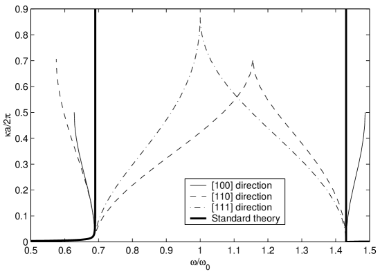
Figure 1: Dispersion relation for three different directions of propagation of a plane wave in a cubic lattice with $a=2r_{B}$ and $\omega_{0}=\omega_{B}$. The polarization for each branch of these curves is described in the text.

As one could expect, one can notice that the predictions of our exact theory depart in a significant way from those of the approximated one as soon as $\kappa a/2\pi$ becomes of order of magnitude comparable to unity. This situation of course corresponds to the fact that the lattice parameter is no longer negligible with respect to the wavelength. A new feature which is revealed by the exact theory is the appearance, even for a perfect cubic lattice, of an anisotropic behavior, consisting in a remarkable dependence of the dispersion relation on the direction of propagation and polarization of the plane waves. The two thin solid curves at the opposite sides of the figure, which both refer to the direction of propagation $[100]$, correspond to transversal (the lower frequency one) and longitudinal polarization respectively. If one considers the dependence of $\omega$ as a function of $\kappa$ which is described by the former curve, one can see that the frequency reaches a maximum — which corresponds to a zero of the group velocity $d\omega/d\kappa$ — and then slowly decreases over a wide region of the $\kappa$ axis extending until the edge of the Brillouin zone. This means that there exists a relatively small interval of the frequency axis with the property that, for each $\omega$ belonging to this interval, there are two transversal modes with direction of propagation along a crystal axis and different values of the wavelength.

A similar phenomenon occurs also for the lowest-frequency branch of the dashed curve, which corresponds to a wave again polarized along a crystal axis, but propagating along the $[110]$ direction. A completely different dispersion relation is shown instead by a wave propagating in the same direction, but transversely polarized along the $[1\bar{1}0]$ direction. This is illustrated by the intermediate branch of the dashed line. For this curve the frequency monotonically increases with $\kappa$ over the entire Brillouin zone, but with a slope — and therefore a group velocity of the associated waves — which drops to a relatively small value when $\omega$ approaches and then exceeds $\omega_{a}$. At the edge of the Brillouin zone this branch joins continuously, at a point with vertical tangent, the third branch of the same curve, which corresponds to longitudinal polarization. This branch extends up to $\omega_{l}$, where a new transversal branch begins. It follows that, at distinction with the modes propagating along the $[100]$ direction, there is no forbidden frequency zone for waves propagating along the $[110]$ direction. Of course, no hint about the existence of such a phenomenon could have been derived from the standard theory. A very similar behavior is shown by the dash-dot curve, corresponding to waves propagating along the $[111]$ direction. Here again the branch with transversal and that with longitudinal polarization join continuously at the edge of the Brillouin zone. Note that, whereas a wave propagating along the $[110]$ direction can be transversely polarized along two directions (the $[001]$ and $[1\bar{1}0]$) with distinct symmetry properties and so also with different dispersion relations, the two possible transversal polarizations are degenerate for waves propagating along either the $[100]$ or $[111]$ directions.

For all the curves displayed in Fig. 1, the polarization vector ${\bf C}$ is either parallel or orthogonal to the wavevector ${\bf q}$. We would like to point out however that this fact is not a general property of the the solutions of Eq. (68), but is rather a consequence of the special symmetry of the particular directions of propagation that we have considered. Note also that the continuous links between the transversal and the longitudinal branches of the curves can be seen as an obvious consequence of the particular degeneracy of the matrix ${\bf\hat{M}}^{(+)}({\bf q},f)$ when ${\bf q}=(\frac{1}{2},\frac{1}{2},0)$ and ${\bf q}=(\frac{1}{2},\frac{1}{2},\frac{1}{2})$.

VII Concluding remarks

In this paper we have presented a new refined version of the classical dispersion theory of electromagnetic radiation in a crystalline solid, which has been completely described at a microscopic level as an infinite regular array of charged oscillators, without ever making use of the continuum approximation. It has been shown that, when the wavelength is comparable with the lattice parameter, the predictions provided by our calculations differ in a remarkable way from those derived from the old standard approximated formulas. In particular, in the region near the proper frequency of the oscillators, which was believed to represent a forbidden gap for light propagation, the phenomenon of “slow light” (i.e. light propagation with small group velocity) is found instead to take place along appropriate crystal directions.

The model we have studied is however interesting in itself also from a purely theoretical point of view, independently of its phenomenological implications. It is in fact an exceptional case of a completely solvable model (although in the dipole approximation) in which the radiation reaction force acting on classical charged point particles is fully taken into account. Actually, it turns out that the inclusion of this force has fundamental implications on the qualitative properties of the solutions, allowing for the existence of undamped collective oscillations. Another interesting feature is that, although the model was formulated in terms of the usual Maxwell–Lorentz electrodynamics with Lorentz–Dirac selfinteraction, it is also compatible with the action-at-a-distance electrodynamics which was proposed by Wheeler and Feynman in 1945 WF . In fact, when the Wheeler–Feynman identity is verified, the two theories lead to the same equations of motion for the charged particles.

Of course the investigations that we have presented here can be developed and extended in several directions. One of these, which appears to be particularly significant also from a phenomenological point of view, is the study of the behavior of a semi-infinite lattice occupying only one half of the full three-dimensional space. This investigation should clarify the relationship between the normal modes of the crystal — which we have described in the present work — and the observable electromagnetic radiation propagating in the free half-space, i.e. the phenomena of refraction and reflection at the surface of the crystal. In this way it is to be expected that classical fundamental results, such as the Ewald–Oseen extinction theorem oseen2 ; oseen3 ; ewald4 ; fearn , will be justified on the basis of the detailed microscopic dynamics of the complete system.

Appendix A Series evaluation

Let us introduce the operator $\hat{C}_{\tau}$, which acts on the generic function $f({\bf k})$ by operating the convolution with a gaussian of width $\sqrt{2\tau}$:

$$[\hat{C}_{\tau}f]({\bf p})=\int d^{3}{\bf k}\frac{\exp(-|{\bf p}-{\bf k}|^{2}/4\tau)}{8(\pi\tau)^{3/2}}f({\bf k})\,.$$

According to Eq. (38), if $f$ is continuous in ${\bf p}$, then $\lim_{\tau\rightarrow 0^{+}}[\hat{C}_{\tau}f]({\bf p})=f({\bf p})$. Furthermore we have for any $f$

$$[\hat{F}\hat{C}_{\tau}f]({\bf x})=e^{-\tau{\bf x}^{2}}[\hat{F}f]({\bf x})\,.$$

The function $b_{ij}^{(0)}({\bf k},\eta)$, defined by Eq. (46), is continuous for ${\bf k}\neq{\bf 0}$ and we have

$$[\hat{C}_{\tau}b_{ij}^{(0)}]({\bf 0},\eta)=\int d^{3}{\bf k}\frac{\exp(-{\bf k}^{2}/4\tau)}{8(\pi\tau)^{3/2}}b_{ij}^{(0)}({\bf k},\eta)=0\,.$$

Therefore, applying Eq. (44) to the function $\hat{C}_{\tau}b_{ij}^{(0)}$, we can write

$$\sum_{{\bf m}\neq{\bf 0}}b_{ij}^{(0)}({\bf H}_{{\bf m}},\eta)$$ (69)

$$= \lim_{\tau\rightarrow 0^{+}}\sum_{{\bf m}}[\hat{C}_{\tau}b_{ij}^{(0)}]({\bf H}_{{\bf m}},\eta)$$

$$= \lim_{\tau\rightarrow 0^{+}}\sum_{{\bf n}}[\hat{F}\hat{C}_{\tau}b_{ij}^{(0)}](2\pi{\bf y}_{{\bf n}},\eta)$$

$$= \lim_{\tau\rightarrow 0^{+}}\sum_{{\bf n}}e^{-\tau{\bf y}_{{\bf n}}^{2}}[\hat{F}b_{ij}^{(0)}](2\pi{\bf y}_{{\bf n}},\eta)\,.$$

Using the formula

$$\frac{1}{(2\pi)^{3}}\int d^{3}{\bf k\,}\frac{e^{i{\bf k}\cdot{\bf x}}}{{\bf k}^{2}}=\frac{1}{4\pi x}\,,$$

with standard arguments it is easy to show that

$$\frac{1}{(2\pi)^{3}}[\hat{F}b_{ij}^{(0)}]({\bf x},\eta)\rightarrow-\frac{3}{4\pi x^{5}}P_{ij}^{(2)}({\bf x})+O(\eta^{\infty})$$

for $\eta\rightarrow 0^{+}$, ${\bf x}\neq{\bf 0}$, while according to Eq. (50)

$$[\hat{F}b_{ij}^{(0)}]({\bf 0},\eta)=\int d^{3}{\bf k}\,b_{ij}^{(0)}({\bf k},\eta)=0\,.$$

Therefore from Eq. (69) one deduces immediately Eqs. (47) and (48). In a very similar way, by the same argument we used to deduce Eq. (64) we have

$$[\hat{C}_{\tau}b_{ijhl}^{(0)}]({\bf 0},\eta) = 0$$

$$\small[\hat{F}b_{ijhl}^{(0)}\small]({\bf 0},\eta) = 0\,,$$

whereas one can show that

$$\frac{1}{(2\pi)^{3}}[\hat{F}b_{ijhl}^{(0)}]({\bf x},\eta) \rightarrow \frac{15}{8\pi x^{7}}P_{ijhl}^{(4)}({\bf x})\left(1-14\frac{\eta}{x^{2}}\right)$$

$$+O(\eta^{\infty})$$

for $\eta\rightarrow 0^{+}$, ${\bf x}\neq{\bf 0}$. Applying again Eq. (44) we then have

$$\sum_{{\bf m}\neq{\bf 0}}b_{ijhl}^{(0)}({\bf H}_{{\bf m}},\eta) = \lim_{\tau\rightarrow 0^{+}}\sum_{{\bf m}}[\hat{C}_{\tau}b_{ijhl}^{(0)}]({\bf H}_{{\bf m}},\eta)$$ (70)

$$= \lim_{\tau\rightarrow 0^{+}}\sum_{{\bf n}}[\hat{F}\hat{C}_{\tau}b_{ijhl}^{(0)}](2\pi{\bf y}_{{\bf n}},\eta)$$

$$= \lim_{\tau\rightarrow 0^{+}}\sum_{{\bf n}}e^{-\tau{\bf y}_{{\bf n}}^{2}}[\hat{F}b_{ijhl}^{(0)}](2\pi{\bf y}_{{\bf n}},\eta)$$

$$= \gamma_{ijhl}^{(0)}-\gamma_{ijhl}^{(-2)}\eta+O(\eta^{\infty})\,,$$

with $\gamma_{ijhl}^{(0)}$ and $\gamma_{ijhl}^{(-2)}$ given by Eqs. (60) and (61) respectively. Hence, by integrating with respect to $\eta$, Eq. (59) is finally obtained.

Appendix B Calculation of $\bar{I}_{ij}$

We have

$$\bar{I}_{ij}({\bf q},f) = \int d^{3}{\bf k\,}\bar{c}_{ij}({\bf k},{\bf q},f)$$ (71)

$$= \lim_{L\rightarrow\infty}\int_{k<L}d^{3}{\bf k}\,\left(c_{ij}-c_{ij}^{(0)}-c_{ij}^{(-2)}\right)$$

$$= \lim_{L\rightarrow\infty}\bigg{\{}\int_{k<L}d^{3}{\bf k}\,c_{ij}({\bf k},{\bf q},f)-\frac{4\pi}{9}L^{3}\delta_{ij}$$

$$-\frac{4\pi}{5}L\left[q_{i}q_{j}-\frac{\delta_{ij}}{3}\left({\bf q}^{2}+10f^{2}\right)\right]\bigg{\}}.$$

Let us put $q=|{\bf q}|$. Since $c_{ij}$ is a second-rank tensor, from invariance considerations it is readily found that we must have

$$\int_{k<L}d^{3}{\bf k}\,c_{ij}({\bf k},{\bf q},f) = \frac{1}{2}A(q,f)\left(\frac{3q_{i}q_{j}}{q^{2}}-\delta_{ij}\right)$$ (72)

$$-\frac{1}{2}B(q,f)\left(\frac{q_{i}q_{j}}{q^{2}}-\delta_{ij}\right)$$

with

$$A(q,f) = \int_{k<L}d^{3}{\bf k}\,c_{ij}({\bf k},{\bf q},f)\frac{q_{i}q_{j}}{q^{2}}$$

$$B(q,f) = \int_{k<L}d^{3}{\bf k}\,c_{ij}({\bf k},{\bf q},f)\delta_{ij}\,.$$

After performing a rotation on the integration space ${\bf k}$, in such a way that the unit vector ${\bf u}_{3}$ of the third coordinate axis is directed along the vector ${\bf q}$, we obtain

$$A(q,f) = \int d^{3}{\bf k}\,\frac{k_{3}^{2}-f^{2}}{k^{2}-f^{2}-i\varepsilon}\theta(L-|{\bf k}-q{\bf u}_{3}|)$$ (73)

$$= -f^{2}LI_{1}(q/L,f/L)$$

$$+L^{3}I_{2}(q/L,f/L)$$

$$B(q,f) = \int d^{3}{\bf k}\,\frac{k^{2}-3f^{2}}{k^{2}-f^{2}-i\varepsilon}\theta(L-|{\bf k}-q{\bf u}_{3}|)$$ (74)

$$= \frac{4}{3}\pi L^{3}-2f^{2}LI_{1}(q/L,f/L)\,,$$

where

$$I_{1}(\bar{q},\bar{f}) = \int d^{3}{\bf k}\,\frac{\theta(1-|{\bf k}-\bar{q}{\bf u}_{3}|)}{k^{2}-\bar{f}^{2}-i\varepsilon}$$

$$I_{2}(\bar{q},\bar{f}) = \int d^{3}{\bf k}\,\frac{k_{3}^{2}\theta(1-|{\bf k}-\bar{q}{\bf u}_{3}|)}{k^{2}-\bar{f}^{2}-i\varepsilon}\,.$$

We have

$$B(0,f) = 3A(0,f)$$ (75)

$$= \frac{4}{3}\pi L^{3}-8\pi f^{2}\left(L+f^{2}\int_{0}^{L}dk\frac{1}{k^{2}-f^{2}-i\varepsilon}\right)$$

$$\rightarrow \frac{4}{3}\pi L^{3}-8\pi f^{2}L-i4\pi^{2}f^{3}$$

for $L\rightarrow\infty$, where we have used the relation

$$\int_{0}^{L}dk\frac{1}{k^{2}-f^{2}-i\varepsilon} \rightarrow \frac{1}{2}\int_{-\infty}^{+\infty}dk\frac{1}{k^{2}-f^{2}-i\varepsilon}$$

$$+O(L^{-1})=\frac{\pi i}{2f}+O(L^{-1})\,.$$

We have also for $\bar{q}=O(L^{-1})$, $\bar{f}=O(L^{-1})$

$$\frac{\partial}{\partial\bar{q}}I_{1}(\bar{q},\bar{f}) = \int d^{3}{\bf k}\,\frac{\delta(1-|{\bf k}-\bar{q}{\bf u}_{3}|)}{k^{2}-\bar{f}^{2}}\frac{k_{3}-\bar{q}}{|{\bf k}-\bar{q}{\bf u}_{3}|}$$

$$= \int d^{3}{\bf k}\,\frac{\delta(1-k)}{k^{2}+2\bar{q}k_{3}+\bar{q}^{2}-\bar{f}^{2}}\frac{k_{3}}{k}$$

$$= 2\pi\int_{-1}^{1}d\xi\frac{\xi}{1+2\bar{q}\xi+\bar{q}^{2}-\bar{f}^{2}}$$

$$= -\frac{8\pi}{3}\bar{q}+O(L^{-3})\,,$$

whence

$$I_{1}(q/L,f/L)=I_{1}(0,f/L)+O(L^{-2})\,.$$ (76)

In a similar way we obtain

$$\frac{\partial}{\partial\bar{q}}I_{2}(\bar{q},\bar{f}) = 2\pi\int_{-1}^{1}d\xi\frac{\xi(\xi+\bar{q})^{2}}{1+2\bar{q}\xi+\bar{q}^{2}-\bar{f}^{2}}$$

$$= \frac{16\pi}{15}\bar{q}+O(L^{-3})\,,$$

so that

$$I_{2}(q/L,f/L)=I_{2}(0,f/L)+\frac{8\pi}{15}\frac{q^{2}}{L^{2}}+O(L^{-4})\,.$$ (77)

From Eqs. (73-77) we get

$$A(q,f) = \frac{4\pi}{9}L^{3}+\frac{8\pi}{3}\left(\frac{q^{2}}{5}-f^{2}\right)L$$

$$-i\frac{4}{3}\pi^{2}f^{3}+O(L^{-1})$$

$$B(q,f) = \frac{4\pi}{3}L^{3}-8\pi f^{2}L-i4\pi^{2}f^{3}+O(L^{-1})\,,$$

then by substituting these expressions into Eqs. (72) and (71) we finally obtain Eq. (65).

References

• (1) M. Born, “Atomtheorie des festen Zustandes,” Teubner, Leipzig, 1923.
• (2) M. Born and E. Wolf, “Principles of Optics,” Pergamon Press, Oxford, 1980.
• (3) H. A. Lorentz, Wiedem. Ann. 9, 641 (1880).
• (4) H. A. Lorentz, Arch. néerland. 25, 363 (1892).
• (5) H. A. Lorentz, “Versuch einer Theorie der elektrischen und optischen Erscheinungen,” Leiden, 1895.
• (6) H. A. Lorentz, “The Theory of Electrons,” Teubner, Leipzig, 1916.
• (7) M. Planck, Berl. Ber. 24, 470 (1902).
• (8) L. Lorenz, Wiedem. Ann. 11, 70 (1881).
• (9) P. P. Ewald, Dissertation, München, 1912.
• (10) P. P. Ewald, Ann. d. Phys. 49, 1 (1916).
• (11) M. Born, “Dynamik der Kristallgitter”, Leipzig, 1915.
• (12) P. P. Ewald, Ann. d. Phys 54, 519 (1917).
• (13) P. A. M. Dirac, Proc. Roy. Soc. London A 167, 148 (1938).
• (14) A. Carati and L. Galgani, Nuovo Cim. B 118, 839 (2003).
• (15) J. A. Wheeler and R. P. Feynman, Rev. Mod. Phys. 17, 157 (1945).
• (16) C. Kittel, “Introduction to Solid State Physics,” 6th ed., Chapters 1 and 2, John Wiley & Sons, New York, 1986.
• (17) R. Becker, “Electromagnetic Fields and Interactions,” vol. II, sec. 40-41, Dover, New York, 1964.
• (18) J. D. Jackson, “Classical Electrodynamics,” 2nd ed., sec. 12.11, John Wiley & Sons, New York, 1975.
• (19) P. W. Milonni and R. W. Boyd, Phys. Rev. A 69, 023814 (2004).
• (20) M. Marino, Annals Phys. 301, 85 (2002).
• (21) C. W. Oseen, Phys. Zeitschr. 17, 341 (1916).
• (22) T. H. Havelock, Proc. Roy. Soc. London 77, 170 (1906); 80, 28 (1907).
• (23) C. W. Oseen, Ann. d. Phys. 48, 1 (1915).
• (24) C. W. Oseen, Phys. Zeitschr. 16, 404 (1915).
• (25) P. P. Ewald, Ann. d. Phys 49, 117 (1916).
• (26) H. Fearn, D. F. V. James and P. W. Milonni, Am. J. Phys. 64, 986 (1996).