Clustering of Aerosols in Atmospheric Turbulent Flow

Abstract

A mechanism of formation of small-scale inhomogeneities in spatial distributions of aerosols and droplets associated with clustering instability in the atmospheric turbulent flow is discussed. The particle clustering is a consequence of a spontaneous breakdown of their homogeneous space distribution due to the clustering instability, and is caused by a combined effect of the particle inertia and a finite correlation time of the turbulent velocity field. In this paper a theoretical approach proposed in Phys. Rev. E 66, 036302 (2002) is further developed and applied to investigate the mechanisms of formation of small-scale aerosol inhomogeneities in the atmospheric turbulent flow. The theory of the particle clustering instability is extended to the case when the particle Stokes time is larger than the Kolmogorov time scale, but is much smaller than the correlation time at the integral scale of turbulence. We determined the criterion of the clustering instability for the Stokes number larger than 1. We discussed applications of the analyzed effects to the dynamics of aerosols and droplets in the atmospheric turbulent flow.

Keywords: Turbulent transport of aerosols and droplets; Atmospheric turbulent flow; Particle clustering instability

I Introduction

It is known that turbulence enhances mixing (see, e.g., MY75 ; C80 ; PS83 ; MC90 ; S96 ; B97 ; W00 ; S01 ; BH03 ). However, numerical simulations, laboratory experiments and observations in the atmospheric turbulence revealed formation of long-living inhomogeneities in spatial distribution of aerosols and droplets in turbulent fluid flows (see, e.g., WM93 ; KM93 ; EF94 ; FK94 ; MC96 ; SC97 ; KS01 ; AC02 ; S03 ; CK04 ; CC05 ; AG06 ). The origin of these inhomogeneities is not always clear but their influence on the mixing can be hardly overestimated.

It is hypothesized that the atmospheric turbulence enhances the rate of droplet collisions (see, e.g., S03 ; PKK97 ; VY00 ; PK00 ; RC00 ). In particular, the turbulence causes formation of small-scale droplet inhomogeneities, and it also increases the relative droplet velocity. In addition, the turbulence affects the hydrodynamic droplet interaction. The latter increases the rate of droplet collisions. These effects are of a great importance for understanding of rain formation in atmospheric clouds. In particular, these effects can cause the droplet spectrum broadening and acceleration of raindrop formation S03 ; VY00 . Note that clouds are known as zones of enhanced turbulence. The preferential concentration of inertial particles (particle clustering) was recently studied in numerical simulations in HC01 ; B03 ; BL04 . The formation of network-like regions of high particle number density was found in BL04 in high resolution direct numerical simulations of inertial particles in a two-dimensional turbulence.

The goal of this study is to analyze the particle-fluid interaction leading to the formation of strong inhomogeneities of aerosol distribution due to a particle clustering instability. The particle clustering instability is a consequence of a spontaneous breakdown of their homogeneous space distribution. As a result, at the nonlinear stage of the clustering instability, the local density of aerosols may rise by orders of magnitude and strongly increase the probability of particle-particle collisions.

It was suggested in EKA96 ; EKB96 ; EK98 that the main cause of the particle clustering instability is their inertia: the particles inside the turbulent eddies are carried out to the boundary regions between the eddies by the inertial forces. This mechanism of the preferential concentration acts in all scales of turbulence, increasing toward small scales. Later, this was contested in EKA00 ; EKA01 using the so-called ”Kraichnan model” K68 of turbulent advection by the delta-correlated in time random velocity field, whereby the clustering instability did not occur.

However, it was shown in EK02 that accounting for a finite correlation time of the fluid velocity field results in the clustering instability of inertial particles. Note that the particle inertia results in the compressibility of particle velocity field. The effects of compressibility of the velocity field on formation of small-scale inhomogeneities in spatial distribution of particles were first discussed in K94 ; EK95 . In this study a theoretical approach proposed in EK02 is further developed and applied to investigate the mechanisms of formation of small-scale aerosol inhomogeneities in the atmospheric turbulent flow. In particular, we extended the theory of particle clustering instability to the case when the particle Stokes time is larger than the Kolmogorov time scale, but is much smaller than the correlation time at the integral scale of turbulence.

Remarkably, the particle inertia also results in formation of the large-scale inhomogeneities in the vicinity of the temperature inversion layers due to excitation of the large-scale instability (see EKA96 ; EKA00 ; EKRA00 ). This effect is caused by additional non-diffusive turbulent flux of particles in the vicinity of the temperature inversion (phenomenon of turbulent thermal diffusion). The characteristic time of excitation of the large-scale instability of concentration distribution of aerosols varies in the range from 0.3 to 3 hours depending on the particle size and parameters of the atmospheric turbulent boundary layer and the temperature inversion layer. The phenomenon of turbulent thermal diffusion was recently detected experimentally using two very different turbulent flows created by oscillating grids turbulence generator BEE04 ; EE04 ; EE06 and multi-fan turbulence generator EEK06 for stably and unstably stratified fluid flows.

The paper is organized as follows. In Sec. II we present governing equations and a qualitative analysis of the clustering instability that causes formation of particle clusters in a turbulent flow. In Sec. III we estimate the scalings of the particle velocity in the turbulent fluid for the case when the particle Stokes time is much larger than the Kolmogorov time scale, but is much smaller than the correlation time at the integral scale of turbulence. In Sec. IV we perform a quantitative analysis for the clustering instability of the second moment of particle number density for ${\rm St}>1$, where ${\rm St}$ is the Stokes number. This allows us to generalize the criterion of the clustering instability obtained in EK02 . Finally, in Sec. V we overview the nonlinear effects which lead to saturation of the clustering instability and determine the particle number density in the cluster. In Sec. V we perform numerical estimates for the dynamics of aerosols and droplets in atmospheric turbulent flow. The conclusions are drawn in Sec. VI. The detail analysis of the scalings of the particle velocity in the turbulent fluid is given in Appendix A. The detail analysis of the clustering instability of the inertial particles is given in Appendix B.

II Governing equations and qualitative analysis of particle clustering

To analyze dynamics of particles we use the standard continuous media approximation, introducing the number density field $n(t,\mathbf{r})$ of spherical particles with radius $a$. The particles are advected by an incompressible turbulent velocity field ${\mathbf{u}}(t,\mathbf{r})$. The particle material density $\rho_{p}$ is much larger than the density $\rho$ of the ambient fluid. For inertial particles their velocity ${\mathbf{v}}(t,{\mathbf{r}})\neq{\mathbf{u}}(t,{\mathbf{r}})$ due to the particle inertia and ${\rm div}\,{\mathbf{v}}(t,{\mathbf{r}})\not=0$ (see MC86 ; M87 ). Therefore, the compressibility of the particle velocity field ${\mathbf{v}}(t,{\mathbf{r}})$ must be taken into account. The growth rate of the clustering instability, $\gamma$, is proportional to $\langle|{\rm div}\,{\mathbf{v}}(t,{\mathbf{r}})|^{2}\rangle$ (see EKA96 ; EKB96 ; EK95 ), where $\langle\cdot\rangle$ denotes ensemble average.

Let $\Theta(t,{\mathbf{r}})$ be the deviation of the instantaneous particle number density $n(t,\mathbf{r})$ from its uniform mean value $N\equiv\langle n\rangle$: $\,\Theta(t,{\mathbf{r}})=n(t,\mathbf{r})-N$. The pair correlation function of $\Theta(t,{\mathbf{r}})$ is defined as $\Phi({\mathbf{R}},{\mathbf{r}},t)\equiv\langle\Theta(t,{\mathbf{r+R}})\Theta(t,{\mathbf{r}})\rangle$. For the sake of simplicity we will consider only a spatially homogeneous, isotropic case when $\Phi({\mathbf{R}},{\mathbf{r}},t)$ depends only on the separation distance $R$ and time $t$, i.e., $\Phi(t,{\mathbf{R}},{\mathbf{r}})=\Phi(t,R)$. Clearly, a large increase of $\Phi(t,R)$ above the level of $N^{2}$ can lead to a strong grows in the frequency of the particle collisions.

In the analytical treatment of the problem we use the standard equation for $n(t,\mathbf{r})$:

$$\frac{\partial n(t,\mathbf{r})}{\partial t}+\mathbf{\nabla}\cdot[n(t,\mathbf{r}){\mathbf{v}}(t,{\mathbf{r}})]=D\triangle n(t,\mathbf{r}),$$ (1)

where D is the coefficient of molecular (Brownian) diffusion. We study the case of small yet finite molecular diffusion $D$ of particles. The equation for $\Theta(t,\mathbf{r})$ follows from Eq. (1):

$$\frac{\partial\Theta(t,\mathbf{r})}{\partial t} + [{\mathbf{v}}(t,{\mathbf{r}})\cdot\nabla]\Theta(t,\mathbf{r})=-\Theta(t,\mathbf{r})\,{\rm div}\,{\mathbf{v}}(t,{\mathbf{r}})$$ (2)

$$+D\triangle\Theta(t,\mathbf{r})\ .$$

To study the clustering instability we use Eq. (2) without the source term $\propto-N\,{\rm div}\,{\mathbf{v}}$, describing the effect of an external source of fluctuations. Particle clustering can also occur due to this source of fluctuations of particle number density. Such fluctuations were studied in B03 ; BL04 ; BF01 . In the present study we considered the particle clustering due to the clustering instability. Particle clustering caused by the self-excitation of fluctuations of particle number density (the clustering instability) is much stronger than that due to the source of fluctuations of particle number density.

One can use Eq. (2) to derive equation for $\Phi(t,R)$ by averaging the equation for $\Theta(t,{\mathbf{r+R}})\Theta(t,{\mathbf{r}})$ over statistics of the turbulent velocity field ${\mathbf{v}}(t,{\mathbf{r}})$. In general this procedure is quite involved even for simple models of the advecting velocity fields (see, e.g., EK02 ). Nevertheless, the qualitative understanding of the underlying physics of the clustering instability, leading to both, the exponential growth of $\Phi(t,R)$ and its nonlinear saturation, can be elucidated by a more simple and transparent analysis.

Let us consider turbulent flow with large Reynolds numbers, ${\mathcal{R}}e\gg 1$. Therefore, the characteristic scale $L$ of energy injection (outer scale) is much larger than the length of the dissipation scales (viscous scale $\eta$) $L\gg\eta$. In the so-called inertial interval of scales, where $L>r>\eta$, the statistics of turbulence within the Kolmogorov theory is governed by the only dimensional parameter, $\varepsilon$, the rate of the turbulent energy dissipation. Then, the velocity $u(r)$ of turbulent motion at the characteristic scale $r$ (referred below as r-eddies) may be found by the dimensional reasoning: $u(r)\approx(\varepsilon r)^{1/3}$ (see, e.g., MY75 ; LL87 ; F95 ). Similarly, the turnover time of $r$-eddies, $\tau(r)$, which is of the order of their life time, may be estimated as $\tau(r)\approx r/u(r)\approx\varepsilon^{-1/3}r^{2/3}$.

To elucidate the clustering instability let us consider a cluster of particles with a characteristic scale $\ell$ moving with the velocity ${\mathbf{V}}_{\rm cl}(t)$. The scale $\ell$ is a parameter which governs the growth rate of the clustering instability, $\gamma$. It sets the bounds for two distinct intervals of scales: $L>r>\ell$ and $\ell>r>\eta$. Note also that we cannot consider scales which are smaller than the size of particles. Large $r$-eddies with $r>\ell$ sweep the $\ell$-cluster as a whole and determine the value of ${\mathbf{V}}_{\rm cl}(t)$. This results in the diffusion of the clusters, and eventually affects their distribution in a turbulent flow.

On the other hand, the particles inside the turbulent eddies are carried out to the boundary regions between the eddies by the inertial forces. This mechanism of the preferential concentration acts in all scales of turbulence, increasing toward small scales. The role of small eddies is multi-fold. First, they lead to the turbulent diffusion of the particles within the scale of a cluster size. Second, due to the particle inertia they tend to accumulate particles in the regions with small vorticity, which leads to the preferential concentration of the particles. Third, the particle inertia also causes a transport of fluctuations of particle number density from smaller scales to larger scales, i.e., in regions with larger turbulent diffusion. The latter can decrease the growth rate of the clustering instability. Therefore, the clustering is determined by the competition between these three processes.

Let us introduce a dimensionless parameter $\sigma_{\rm v}$, a degree of compressibility of the velocity field of particles, ${\mathbf{v}}(t,{\mathbf{r}})$, defined by

$$\sigma_{\rm v}\equiv{\langle[{\rm div}\,{\mathbf{v}}]^{2}\rangle\over\langle|\nabla\times{\mathbf{v}}|^{2}\rangle}\ .$$ (3)

This parameter may be of the order of 1 (see EKA00 ). One of the reasons for the clustering instability is the particle inertia which results in the parameter $\sigma_{\rm v}\not=0$. The particle response time is given by

$$\tau_{p}=\frac{m_{p}}{6\pi\,\nu\,\rho\,a}=\frac{2\rho_{p}\,a^{2}}{9\rho\,\nu}\,,$$ (4)

and the particle mass $m_{p}$ is $m_{p}=(4\pi/3)\,a^{3}\,\rho_{p}$. The ratio of the inertial time scale of the particles (the Stokes time scale $\tau_{p}$) and the turnover time of $\eta$-eddies in the Kolmogorov micro-scale $\tau(\eta)=\eta/u(\eta)=\eta^{2}/\nu$, is of primary importance, where $u(\eta)$ is the characteristic velocity of $\eta$-scale eddies. The ratio of the time-scales $\tau_{p}$ and $\tau(\eta)$ is the Stokes number:

$${\rm St}\equiv\frac{\tau_{p}}{\tau(\eta)}=\frac{2\rho_{p}\,a^{2}}{9\rho\,\eta^{2}}\ .$$ (5)

For $\tau_{p}\ll\tau(\eta)$ all particles are almost fully involved in turbulent motion, and one concludes that $u(t,{\mathbf{r}})\approx v(t,{\mathbf{r}})$ and $v(\ell)\approx u(\ell)$. The compressibility parameter $\sigma_{\rm v}$ of particle velocity field for ${\rm St}\ll 1$ is given by:

$$\sigma_{\rm v}\sim\left(\frac{2\rho_{p}}{9\rho}\right)^{2}\left(\frac{a}{\eta}\right)^{4}={\rm St}^{2}\,.$$ (6)

(see EK02 ; EKA00 ). For small Stokes number, the clustering instability has been investigated in EK02 . The characteristic scale of the most unstable clusters of small particles is of the order of Kolmogorov micro-scale of turbulence, $\eta$. The characteristic growth rate of the clustering instability is of the order of the turnover frequency of $\eta$-eddies, $1/\tau(\eta)$ (see EK02 ). In the present study we extend the theory of particle clustering instability to the case ${\rm St}>1$, i.e., when the particle Stokes time is larger than the Kolmogorov time scale, but is much smaller than the correlation time at the integral scale of turbulence. We may expect that for ${\rm St}>1$ the compressibility parameter $\sigma_{\rm v}$ of particle velocity field is given by:

$$\sigma_{\rm v}\sim{{\rm St}^{2}\over 1+\alpha\,{\rm St}^{2}}\,,$$ (7)

where $\alpha\sim 1$.

III The particle velocity field for ${\rm St}\gg 1$

The equation of motion of a particle reads:

$$\frac{d{\mathbf{v}}(t,{\mathbf{r}})}{dt}={1\over\tau_{p}}[{\mathbf{u}}(t,{\mathbf{r}})-{\mathbf{v}}(t,{\mathbf{r}})]\;,$$ (8)

where the total time derivative $(d/dt)$ takes into account the time dependence of the particle coordinate $\mathbf{r}$:

$$\frac{d}{dt}=\left[\frac{\partial}{\partial t}+{\mathbf{v}}(t,{\mathbf{r}})\cdot\nabla\right]\ .$$ (9)

Now Eq. (8) takes the form:

$$\left\{\tau_{p}\left[\frac{\partial}{\partial t}+{\mathbf{v}}(t,{\mathbf{r}})\cdot\nabla\right]+1\right\}{\mathbf{v}}(t,{\mathbf{r}})={\mathbf{u}}(t,{\mathbf{r}})\ .$$ (10)

In the following we analyze this equation for particles with the time $\tau_{p}$ which is larger than the turnover time of the smallest eddies in the Kolmogorov micro-scale $\tau(\eta)$, but is smaller than the turnover time of the largest eddies $\tau(L)$. Denote by $\ell_{*}$ the characteristic scale of eddies for which

$$\tau_{p}=\tau(\ell_{*})\ .$$ (11)

This scale as well as the particle cluster scale was introduced in EKB96 . Note that $\ell_{*}/\eta={\rm St}^{3/2}$. The eddies with $\ell\gg\ell_{*}$ almost fully involve particles in their motions, while the eddies with $\ell\ll\ell_{*}$ do not affect the particle motions in the zero order approximation with respect to the ratio $[\tau(\ell)/\tau_{p}]\ll 1$. Therefore it is conceivable to suggest that the main contribution to the particle velocity is due to the eddies with the scale of $\ell$ [which we denote as ${\bm{v}}_{\ell}(t,{\bm{r}})$] that is of the order of $\ell_{*}$ and much larger then the Kolmogorov micro-scale. Velocity ${\bm{v}}_{\ell}(t,{\bm{r}})$ cannot be found on the basis of simple dimensional reasoning because the problem at hand involves a number of dimensionless parameters like $\ell/\ell_{*}$, $\ell_{*}/\eta$, etc. The main difficultly in determining this velocity is that in this case one has to take into account for a modification of the particle response time $\tau_{p}$ by the turbulent fluctuations. The physical reason for that is quite obvious: the time $\tau_{p}$ is determined by molecular viscosity of the carrier fluid while the main dissipative effect for motions with $\ell>\eta$ is due to the effective “turbulent” viscosity. In order to determine the velocity ${\bm{v}}_{\ell}(t,{\bm{r}})$ we can use the perturbation approach to Eq. (10) (see, e.g., LPA95 ; LPB95 ). The details of this derivations are given in Appendix A. This analysis yields the scalings of the particle velocity for ${\rm St}\gg 1$:

$${v}^{2}_{\ell}\approx u^{2}_{\ell}\left(\frac{\ell}{\ell_{*}}\right)^{10/9}\approx u^{2}_{\ell}\left[\frac{\tau(\ell)}{\tau_{p}}\right]^{5/3}\ .$$ (12)

IV The clustering instability of the second moment of particle number density

In this section we will perform a quantitative analysis for the clustering instability of the second moment of particle number density. To determine the growth rate of the clustering instability let us consider the equation for the two-point correlation function $\Phi(t,{\bm{R}})$ of particle number density:

$${\partial\Phi\over\partial t}=[B({\bm{R}})+2{{\bm{U}}}({\bm{R}})\cdot{\bm{\nabla}}+\hat{D}_{\alpha\beta}({\bm{R}})\nabla_{\alpha}\nabla_{\beta}]\,\Phi(t,{\bm{R}})\,,$$ (13)

(see EK02 ). The meaning of the coefficients $B({\bm{R}})$, ${\bm{U}}({\bm{R}})$ and $\hat{D}_{\alpha\beta}({\bm{R}})$ is as follows (for details see Appendix B). The function $B({\bm{R}})$ is determined by the compressibility of the particle velocity field and it causes the generation of fluctuations of the number density of particles. The vector ${\bm{U}}({\bm{R}})$ determines a scale-dependent drift velocity which describes a transport of fluctuations of particle number density from smaller scales to larger scales, i.e., in the regions with larger turbulent diffusion. The latter can decrease the growth rate of the clustering instability. Note that ${\bf U}({\bm{R}}=0)=0$ whereas $B({\bm{R}}=0)\not=0.$ For incompressible velocity field ${\bf U}({\bm{R}})=0$ and $B({\bm{R}})=0$. The scale-dependent tensor of turbulent diffusion $\hat{D}_{\alpha\beta}({\bm{R}})$ is also affected by the compressibility. In very small scales this tensor is equal to the tensor of the molecular (Brownian) diffusion, while in the vicinity of the maximum scale of turbulent motions this tensor coincides with the regular tensor of turbulent diffusion.

Thus, the clustering instability is determined by the competition between these three processes. The form of the coefficients $B({\bm{R}})$, ${\bm{U}}({\bm{R}})$ and $\hat{D}_{\alpha\beta}({\bm{R}})$ depends on the model of turbulent velocity field. For instance, for the random velocity with Gaussian statistics of the particle trajectories these coefficients are given in Appendix B.

Let us study the clustering instability. We consider particles with the size $\eta/\sqrt{\rm Sc}\ll a\ll\eta$, where ${\rm Sc}=\nu/D$ is the Schmidt number. For small inertial particles advected by air flow ${\rm Sc}\gg 1$. There are three characteristic ranges of scales, where the form of the solution of Eq. (13) for the two-point correlation function $\Phi(t,{\bm{R}})$ of the particle number density is different. These ranges of scales are the following: (i) the dissipative range $a\leq\ell\leq\eta$, where the molecular diffusion term $\propto 1/{\rm Sc}$ is negligible; (ii) the first part of the inertial range $\eta\leq\ell\leq\ell_{\ast}$ and (iii) the second part of the inertial range $\ell_{\ast}\ll\ell\ll L$, where the functions $B({\bm{R}})$ and ${\bm{U}}({\bm{R}})$ are negligibly small.

Consider a solution of Eq. (13) in the vicinity of the thresholds of the excitation of the clustering instability. The asymptotic solution of the equation for the two-point correlation function $\Phi(t,{\bm{R}})$ of the particle number density is obtained in Appendix B. In the range of scales $a\leq\ell\leq\eta$, the correlation function $\Phi(t,{\bm{R}})$ in a non-dimensional form reads

$$\Phi(R)=A_{1}R^{-\lambda_{d}}\sin(\mu_{d}|\ln\,R|+\varphi_{d})\,,$$ (14)

and in the range of scales $\eta\leq\ell\leq\ell_{\ast}$ it is given by

$$\Phi(R)=A_{2}R^{-\lambda}\sin(\mu\ln\,R+\varphi)\,,$$ (15)

where the parameters $\lambda_{d}$ and $\mu_{d}$ are given by Eq. (B.59) and the parameters $\lambda$ and $\mu$ are given by Eq. (B.64) in Appendix B. Here $R$ is measured in the units of $\eta$ and time $t$ is measured in the units of $\tau_{\eta}\equiv\tau(\ell=\eta)$. We have taken into account that the correlation function $\Phi(R)$ has a global maximum at $R=a$, i.e. the normalized correlation function of the particle number density $\Phi(t,R=a)=1$. We have also taken into account that in the range of scales $\eta\leq\ell\ll\ell_{\ast}$, the relationship between $v^{2}_{\ell}$ and $u^{2}_{\ell}$ is given by:

$$v^{2}_{\ell}=u^{2}_{\ell}\left[\frac{\tau(\ell)}{\tau_{p}}\right]^{s}\ .$$ (16)

For instance, for ${\rm St}\gg 1$ the exponent $s=5/3$ (see Eq. (12)). The value $s=7/4$ corresponds to the turbulent diffusion tensor with the scaling $\propto R^{2}$ [see Eqs. (B.56)-(B.58) in Appendix B]. We consider the parameter $s$ as a phenomenological parameter. In the range of scales $\ell_{\ast}\ll\ell\ll L$, the correlation function $\Phi(t,{\bm{R}})$ is given by

$$\Phi(R)=A_{3}R^{-\lambda_{3}}\,,$$ (17)

where $\lambda_{3}$ is given by Eq. (B.68) in Appendix B. The condition, $\int_{0}^{\infty}R^{2}\Phi(R)\,dR=0$, implies that the total number of particles in a closed volume is conserved.

The growth rate of the second moment of particle number density, the coefficients $A_{k}$ and the parameters $\varphi_{d}$, $\varphi$ are determined by matching the correlation function $\Phi(R)$ and its first derivative $\Phi^{\prime}(R)$ at the boundary of the above three ranges of scales, i.e., at the points $\ell=\eta$ and $\ell=\ell_{\ast}.$ For example, the growth rate $\gamma$ of the clustering instability of the second-order correlation function is given by

$$\gamma = {1\over 6\,\tau_{\eta}(1+3\sigma_{{}_{T}})}\biggl{[}400\,\sigma_{\rm v}\,{\sigma_{{}_{T}}-\sigma_{\rm v}\over 1+\sigma_{\rm v}}-{(3-\sigma_{{}_{T}})^{2}\over 1+\sigma_{{}_{T}}}$$ (18)

$$-4\mu_{d}^{2}\,{(1+3\sigma_{{}_{T}})^{2}\over 1+\sigma_{{}_{T}}}\biggr{]}\;,$$

where $\sigma_{{}_{T}}$ is the degree of compressibility of the scale-dependent tensor of turbulent diffusion $\hat{D}_{\alpha\beta}({\bm{R}})$ (for details, see Appendix B). Note that for the $\delta$-correlated in time random Gaussian compressible velocity field, the coefficients $B({\bm{R}})$ and ${\bm{U}}({\bm{R}})$ are related to the turbulent diffusion tensor $\hat{D}_{\alpha\beta}({\bm{R}})$, i.e.,

$$B({\bm{R}})=\nabla_{\alpha}\nabla_{\beta}\hat{D}_{\alpha\beta}({\bm{R}})\,,\quad U_{\alpha}({\bm{R}})=\nabla_{\beta}\hat{D}_{\alpha\beta}({\bm{R}})\,,$$ (19)

(for details, see EKA00 ; EKA01 ; EK02 ). In this case the second moment $\Phi(t,{\bm{R}})$ can only decay, in spite of the compressibility of the velocity field. For the $\delta$-correlated in time random Gaussian compressible velocity field $\sigma_{\rm v}=\sigma_{{}_{T}}$. For the finite correlation time of the turbulent velocity field $\sigma_{{}_{T}}\not=\sigma_{\rm v}$ and the relationships (19) are not valid. The clustering instability depends on the ratio $\sigma_{{}_{T}}/\sigma_{\rm v}$.

The range of parameters $(\sigma_{\rm v},\sigma_{{}_{T}})$ for which the clustering instability of the second moment of particle number density may occur is shown in Fig. 1. The line $\sigma_{\rm v}=\sigma_{{}_{T}}$ corresponds to the $\delta$-correlated in time random compressible velocity field for which the clustering instability cannot be excited. The various curves indicate results for different value of the parameter $s$. The curves for $s=7/4$ (dashed) and $s=5/3$ (solid) practically coincide. The parameter $s$ is considered as a phenomenological parameter, and the change of this parameter from $s=7/4$ to $s=0$ can describe a transition from one asymptotic behaviour (in the range of scales $\eta\leq\ell\leq\ell_{\ast}$) to the other ($\ell_{\ast}\ll\ell\leq L$). The growth rate (18) of the clustering instability versus $\sigma_{\rm v}$ for $s=5/3$ and different values of $\sigma_{{}_{T}}$ is shown in Fig. 2.

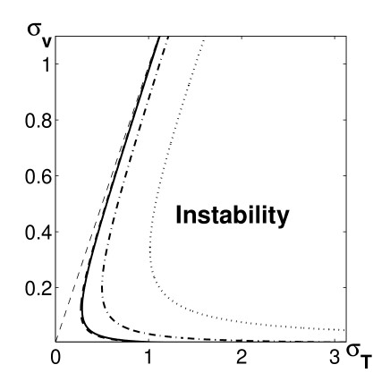
Figure 1: The range of parameters $(\sigma_{\rm v},\sigma_{{}_{T}})$ for which the clustering instability may occur. The various curves indicate results for $s=7/4$ (dashed), $s=5/3$ (solid), for $s=1$ (dashed-dotted) and for $s=2/3$ (dotted). The thin dashed line $\sigma_{\rm v}=\sigma_{{}_{T}}$ corresponds to the $\delta$-correlated in time random compressible velocity field.

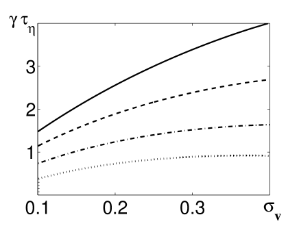
Figure 2: The growth rate of the clustering instability versus $\sigma_{\rm v}$ for $s=5/3$. The various curves indicate results for different values of $\sigma_{{}_{T}}=\sigma_{\rm v}+\delta$: $\;\delta=3$ (solid), $\,\delta=1$ (dashed), $\delta=0.5$ (dashed-dotted) and $\delta=0.3$ (dotted).

We have not discussed in the present study the growth of the high-order moments of particle number density (see EKB96 ; EK02 ; BF01 ; ZM88 ). The growth of the negative moments of particles number density (possibly associated with formation of voids and cellular structures) was discussed in BF01 ; SZ89 ; KS97 .

V Discussion

Formation and evolution of particle clusters are of fundamental significance in many areas of environmental sciences, physics of the atmosphere and meteorology [smog and fog formation, rain formation (see e.g., S86 ; FS88 ; PK97 ; KS01 ; CK04 ; CC05 ), planetary physics (see e.g., HB98 ; BC99 ), transport and mixing in industrial turbulent flows, like spray drying and cyclone dust separation, dynamics of fuel droplets (see e.g., CS98 ; H88 ; BR99 ). The analysis of the experimental data showed that the spatial distributions of droplets in clouds are strongly inhomogeneous (see S03 ). The small-scale inhomogeneities in particle distribution were observed also in laboratory turbulent flows (see FK94 ; AC02 ; AG06 ).

In the present study we have shown that the particle spatial distribution in the turbulent flow field is unstable against formation of clusters with particle number density that is much higher than the average particle number density. Obviously this exponential growth at the linear stage of instability should be saturated by nonlinear effects. A momentum coupling of particles and turbulent fluid is essential when the kinetic energy of fluid $\rho\langle{{\bm{u}}}^{2}\rangle$ is of the order of the particles kinetic energy $m_{\rm p}n_{\rm cl}\langle{{\bm{v}}}^{2}\rangle,$ where $|{{\bm{u}}}|\sim|{{\bm{v}}}|$, i.e., when $m_{\rm p}n_{\rm cl}\sim\rho$. This condition implies that the number density of particles in the cluster $n_{\rm cl}\sim a^{-3}(\rho/3\rho_{\rm p})$. In the atmospheric turbulence the characteristic parameters are as follows: in the viscous scale, $\eta\sim 1$ mm, the correlation time of the turbulent velocity field is $\tau_{\eta}\sim(0.01-0.1)$ s, and for water droplets $\rho_{\rm p}/\rho\sim 10^{3}$. Thus, for $a\sim 30\,\mu$m we obtain $n_{\rm cl}\sim 10^{4}$ cm^-3 (see EK02 ). Particle collisions can play also essential role when during the life-time of a cluster the total number of collisions is of the order of number of particles in the cluster. The collisions in clusters may be essential for $n_{\rm cl}\sim a^{-3}(\ell_{\ast}/a)(\rho/3\rho_{\rm p})$. In this case a mean separation of particles in the cluster is of the order of $\ell_{\rm s}\sim a^{4/3}(3\rho_{\rm p}/\ell_{\ast}\rho)^{1/3}$. When, e.g., $a\sim 30\,\mu$m we get $\ell_{\rm s}\sim 5\,a\approx 150\,\mu$m and $n_{\rm cl}\sim 3\times(10^{4}-10^{5})$ cm^-3. The mean number density of droplets in clouds $N$ is about $10^{3}$ cm^-3. Therefore, the clustering instability of droplets in clouds can increase their concentrations in the clusters by the order of magnitude (see also EK02 ). Note that for large Stokes numbers the terminal fall velocity of particles can be much larger than the turbulent velocity. This implies that the sedimentation of heavy particles can suppress the clustering instability for large Stokes numbers.

Figure 3: Dependence of $\sqrt{\langle n^{2}\rangle}/N$ versus parameter $\sigma_{\rm v}$ for $s=5/3$ which corresponds to the solution of Eq. (13) for the two-point correlation function $\Phi(t,{\bm{R}})$ of the particle number density obtained in Sec. IV. Various curves indicate results for different values of the parameter $\delta$: $\;\delta=3$ (solid), $\,\delta=1$ (dashed) and $\delta=0.5$ (dashed-dotted), where $\sigma_{{}_{T}}=\sigma_{\rm v}+\delta$.

Figure 4: Dependence of $\sqrt{\langle n^{2}\rangle}/N$ versus parameter $\sigma_{\rm v}$ which corresponds to the solution for the two-point correlation function $\Phi(t,{\bm{R}})$ of the particle number density for the case ${\rm St}<1$ studied in EK02 . Various curves indicate results for different values of the parameter $\delta$: $\;\delta=3$ (solid), $\,\delta=1$ (dashed) and $\delta=0.3$ (dashed-dotted), where $\sigma_{{}_{T}}=\sigma_{\rm v}+\delta$. The thick lines correspond to ${\rm Sc}=10^{5}$ and thin lines correspond to ${\rm Sc}=10^{4}$.

There is an additional restriction on the value of $n_{\rm cl}=\sqrt{\langle n^{2}\rangle}$ which follows from the condition $\langle n(t,\mathbf{r})\,n(t,\mathbf{r}+\mathbf{R})\rangle\equiv N^{2}+\langle\Theta^{2}\rangle\Phi(t,\mathbf{R})\geq 0$, where $\Phi(t,\mathbf{R})$ is the normalized correlation function of the particle number density $\Phi(t,R=a)=1$. Since the correlation function $\Phi(t,\mathbf{R})$ can be negative at some scale $R$, this condition implies that the maximum possible value of $\langle\Theta^{2}\rangle$ which can be achieved during the clustering instability is $\langle\Theta^{2}\rangle_{\rm max}=N^{2}/|\Phi|_{\rm min}$. Therefore, the number density of particles in the cluster $n_{\rm cl}$ cannot be larger than $n_{\rm cl}\leq N(1+|\Phi|_{\rm min}^{-1})^{1/2}$. Using this criterion we plotted in Fig. 3 the dependencies $\sqrt{\langle n^{2}\rangle}_{\rm max}/N$ versus parameter $\sigma_{\rm v}$ for different values of the parameter $\delta$, where $\sigma_{{}_{T}}=\sigma_{\rm v}+\delta$. We estimate $|\Phi|_{\rm min}$ using the solution of Eq. (13) for the two-point correlation function $\Phi(t,{\bm{R}})$ of the particle number density obtained in Sec. IV. Note however, that this solution determines the linear stage of the clustering instability. In Fig. 3 we also take into account the conditions for the clustering instability. This condition implies that for a given parameter $\sigma_{{}_{T}}$ the clustering instability is excited when $\sigma_{\rm v}>\sigma_{\rm v}^{\rm min}$ (see Fig. 1). For comparison we also plotted in Fig. 4 the similar dependencies $\sqrt{\langle n^{2}\rangle}_{\rm max}/N$ versus parameter $\sigma_{\rm v}$ using the solution for the two-point correlation function $\Phi(t,{\bm{R}})$ of the particle number density for the case ${\rm St}<1$ studied in EK02 .

In the present study we have considered the particle clustering due to the clustering instability. Generally, particle clustering can also occur due to the source of fluctuations of droplets number density $I=B({\bf R})N^{2}$ in Eq. (13) for the second-order correlation function of particle number density. This source term arises due to the term $\propto-N\,{\rm div}\,{\bf v}$ in Eq. (2). Such fluctuations were studied in B03 ; BL04 ; BF01 .

Note that there is an alternative approach which determines the particle clustering (see DM05 ; MW05 ; WM05 ). The particle number density fluctuations are generated by a multiplicative random process: volume elements in the particle flow are randomly compressed or expanded, and the ratio of the final density to the initial density after many multiples of the correlation time $\tau$ can be modelled as a product of a large number of random factors. According to this picture, the particle number density fluctuations will be a record of the history of the flow, and may bear no relation to the instantaneous disposition of vortices when the particle number density is measured DM05 ; MW05 ; WM05 . The particle number density is expected to have a log-normal probability distribution. When the random-flow model DM05 ; MW05 ; WM05 with short correlation time is applied to fully-developed turbulence it predicts that the clustering is strongest when ${\rm St}\sim 1$, in agreement with numerical studies CK04 ; CC05 .

VI Conclusions

In this study we considered formation of small-scale clusters of inertial particles in a turbulent flow. The mechanism for particle clustering is associated with a small-scale instability of particle spatial distribution. The clustering instability is caused by a combined effect of the particle inertia and a finite correlation time of the turbulent velocity field. The theory of particle clustering developed in our previous studies was extended to the case when the particle Stokes time is larger than the Kolmogorov time scale, but is much smaller than the correlation time at the integral scale of turbulence. We found the criterion for the clustering instability for this case.

Acknowledgments

This research was supported in part by The German-Israeli Project Cooperation (DIP) administrated by the Federal Ministry of Education and Research (BMBF), by the Israel Science Foundation governed by the Israeli Academy of Science, by Binational Israel - United States Science Foundation (BSF), by the Israeli Universities Budget Planning Committee (VATAT) and Israeli Atomic Energy Commission, by Swedish Ministry of Industry (Energimyndigheten, contract P 12503-1), by the Swedish Royal Academy of Sciences, the STINT Fellowship program.

Appendix A Velocity of inertial particles for $\tau_{p}\gg\tau_{\eta}$

In order to determine the velocity ${\bm{v}}_{\ell}(t,{\bm{r}})$ we can use the Wyld’s perturbation diagrammatic approach to Eq. (10) in the Belinicher-L’vov representation (see, e.g., LPA95 ; LPB95 ). This approach yields automatically a sensible result allowing us to avoid an overestimation of the sweeping effect in an order-by-order perturbation analysis. However, keeping in mind that this approach is technically quite involved, in this study we reformulated the derivation procedure and obtained the required results using a more simple procedure based on the equation of motion Eq. (10).

To determine ${\bm{v}}_{\ell}(t,{\bm{r}})$ we consider Eq. (10) in the frame moving with $\ell$-eddies, in which the surrounding fluid velocity ${\bm{u}}$ equals to the relative velocity of the $\ell$-eddy at ${\bm{r}}$, i.e., ${\bm{u}}(t,{\bm{r}})={\bm{u}}_{\ell}(t,{\bm{r}})$. Here one has to take into account that the $\ell$-eddy is swept out by all eddies with scales $\ell^{\prime}>\ell$. At the same time the particles participate in motions of $\ell^{\prime}$-eddies with $\ell^{\prime}>\ell_{*}>\ell$. Therefore, the relative velocity ${\bm{v}}_{\ell}$ of the $\ell$-eddy and the particle is determined by $\ell^{\prime}$-eddies with the intermediate scales, $\ell_{*}\leq\ell^{\prime}\leq\ell$. This velocity is determined by the contribution of $\ell_{*}$-eddies, and can be considered as a time and space independent constant ${\bm{u}}_{*}$ during the life time of the $\ell$ eddy and inside it. Velocity ${\bm{u}}_{*}$ in our approach is random and has the same statistics as the statistics of the turbulent velocities of $\ell_{*}$-eddies. Then Eq. (10) becomes

$$\left(\tau_{p}\frac{\partial}{\partial t}+1\right){\bm{v}}_{\ell}(t,{\bm{r}})={\bm{u}}_{\ell}(t,{\bm{r}+{\bm{u}}_{*}t})$$

$$\quad\quad-\tau_{p}\left[{\bm{v}}_{\ell}(t,{\bm{r}})\cdot\nabla\right]{\bm{v}}_{\ell}(t,{\bm{r}})\ .$$ (A.20)

In Eq. (A.20) the velocity ${\bm{u}}_{\ell}$ is calculated at point ${\bm{r}}$ and the velocity ${\bm{v}}_{\ell}$ is at ${\bm{r}}-{\bm{u}}_{*}\,t$. For the sake of convenience we redefine here ${\bm{r}}-{\bm{u}}_{*}\,t={\bm{r}}^{\prime}$ as ${\bm{r}}$ and, respectively, ${\bm{r}}={\bm{r}}^{\prime}+{\bm{u}}_{*}\,t$ as ${\bm{r}}+{\bm{u}}_{*}\,t$. Note that Eq. (A.20) is a simplified version of Eq. (10) that we used in our derivations.

A.1 First non-vanishing contribution to $v_{\ell}$

Since $v_{\ell}(t,{\bm{r}})\ll u_{\ell}$ for $\ell\ll\ell_{*}$, we can find the first non-vanishing contribution to ${\bm{v}}_{\ell}(t,{\bm{r}})$ in the limit $[\tau(\ell)\ll\tau_{p}]$ by considering the linear version of Eq. (A.20):

$$\left(\tau_{p}\frac{\partial}{\partial t}+1\right){\bm{v}}_{\ell}(t,{\bm{r}})={\bm{u}}_{\ell}(t,{\bm{r}}+{\bm{u}}_{*}t)\ .$$ (A.21)

In the $\omega,{\bm{k}}$ representation this equation takes the form:

$$\left(i\omega\,\tau_{p}+1\right){\bm{v}}_{\ell}(\omega,{\bm{k}})={\bm{u}}_{\ell}(\omega-{\bm{k}}\cdot{\bm{u}}_{*},{\bm{k}})\,,$$ (A.22)

that allows one to find the relationship between the second order correlation functions $F_{v,\ell}^{\alpha\beta}(\omega,{\bm{k}})$ and $F_{u,\ell}^{\alpha\beta}(\omega,{\bm{k}})$ of the velocity fields ${\bm{v}}_{\ell}$ and ${\bm{u}}_{\ell}$:

$$F_{v,\ell}^{\alpha\beta}(\omega,{\bm{k}})=\frac{1}{\omega^{2}\tau_{p}^{2}+1}F_{u,\ell}^{\alpha\beta}(\omega-{\bm{k}}\cdot{\bm{u}}_{*},{\bm{k}})\ .$$ (A.23)

Functions $F_{u,\ell}^{\alpha\beta}(\omega,{\bm{k}})$ and $F_{v,\ell}^{\alpha\beta}(\omega,{\bm{k}})$ are defined as usual, e.g.,

$$(2\pi)^{4}\delta(\omega+\omega^{\prime})\,\delta({\bm{k}}+{\bm{k}}^{\prime})F_{u,\ell}^{\alpha\beta}(\omega,{\bm{k}})\equiv$$

$$\left\langle v_{\ell}^{\alpha}(\omega,{\bm{k}})\,v_{\ell}^{\beta}(\omega^{\prime},{\bm{k}}^{\prime})\right\rangle\;.$$ (A.24)

The simultaneous correlation functions are related to their $\omega$-dependent counterparts via the integral $\int d\omega/2\pi$, e.g.,

$$F_{v,\ell}^{\alpha\beta}({\bm{k}})=\int\frac{d\omega}{2\pi}F_{v,\ell}^{\alpha\beta}(\omega,{\bm{k}})\ .$$ (A.25)

The tensorial structure of $F_{u,\ell}^{\alpha\beta}({\bm{k}})$ follows from the incompressibility condition and the assumption of isotropy:

$$F_{u,\ell}^{\alpha\beta}({\bm{k}})=P^{\alpha\beta}({\bm{k}})F_{u,\ell}(k)\,,$$ (A.26)

where $P^{\alpha\beta}({\bm{k}})$ is the transversal projector:

$$P^{\alpha\beta}({\bm{k}})=\delta_{\alpha\beta}-k^{\alpha}k^{\beta}/k^{2}\ .$$ (A.27)

In the inertial range of scales the function $F_{u,\ell}^{\alpha\beta}(\omega,{\bm{k}})$ may be written in the following form:

$$F_{u,\ell}^{\alpha\beta}(\omega,{\bm{k}})=P^{\alpha\beta}({\bm{k}})\,F_{u,\ell}(k)\,\tau(\ell)\,f[\omega\,\tau(\ell)]\ .$$ (A.28)

Here the dimensionless function $f(x)$ is normalized as follows:

$$\int_{-\infty}^{\infty}f(x)\,dx=2\pi\ .$$ (A.29)

Now we can average Eq. (A.23) over the statistics of $\ell_{*}$-eddies. Denoting the mean value of some function $g(x)$ as $\overline{g(x)}$ we have:

$$\overline{f[(\omega-{\bm{k}}\cdot{\bm{u}}_{*})\,\tau(\ell)]}\approx\overline{\delta[(\omega-{\bm{k}}\cdot{\bm{u}}_{*})\,\tau(\ell)]}$$

$$\approx\frac{\ell}{\tau(\ell)\,u_{*}}\,f_{*}\left(\frac{u_{*}\,\omega}{\ell}\right)\ .$$ (A.30)

Here the dimensionless function $f_{*}(x)$ has one maximum at $x=0$, and it is normalized according to Eq. (A.29). The particular form of $f_{*}(x)$ depends on the statistics of $\ell_{*}$-eddies and our qualitative analysis is not sensitive to this form. Thus, we may choose, for instance:

$$f_{*}(x)=2/[x^{2}+1]\ .$$ (A.31)

In Eqs. (A.1) we took into account that the characteristic Doppler frequency of $\ell$-eddies (in the random velocity field $u_{*}$ of $\ell_{*}$-eddies) may be evaluated as:

$$\gamma_{{}_{D}}(\ell)\equiv\sqrt{\overline{({\bm{k}}\cdot{\bm{u}}_{*})^{2}}}\simeq u_{*}/\ell\ .$$ (A.32)

This frequency is much larger than the characteristic frequency width of the function $f[\omega\tau(\ell)]$ (equal to $1/\tau(\ell)$), and therefore the function $f(x)$ in Eq. (A.1) may be approximated by the delta function $\delta(x)$.

After averaging, Eq. (A.23) may be written as

$$F_{v,\ell}^{\alpha\beta}(\omega,{\bm{k}})=\frac{P^{\alpha\beta}({\bm{k}})f_{*}(0)}{\omega^{2}\tau_{p}^{2}+1}\frac{\ell}{u_{*}}F_{u,\ell}(k)\ .$$ (A.33)

Here we took into account that $\tau_{p}\gg\ell/u_{*}$ that allows us to neglect the frequency dependence of $f_{*}(u_{*}\,\omega/\ell)$ and to calculate this function at $\omega=0$. Together with Eq. (A.33) this yields

$$F_{v,\ell}^{\alpha\beta}({\bm{k}})=P^{\alpha\beta}({\bm{k}})\,F_{u,\ell}(k)\frac{\,\ell}{\,\tau_{p}\,u_{*}}\,,$$ (A.34)

where we used the estimate $f_{*}(0)\approx 2$, that follows from Eq. (A.31).

The equation (A.34) provides the relationship between the mean square relative velocity of $\ell$-separated particles, $v_{\ell}$, and the velocity of $\ell$-eddies, $u_{\ell}$:

$$v_{\ell}\simeq u_{\ell}\sqrt{\frac{\,\ell}{\,\tau_{p}\,u_{*}}}\simeq u_{\ell}\sqrt{\frac{\,\ell}{\ell_{*}}}\ .$$ (A.35)

A.2 Effective nonlinear equation

For a qualitative analysis of the role of the nonlinearity of the particle behavior in the $\ell$-cluster we evaluate $\nabla$ in the nonlinear term, Eq. (A.20), as $1/\ell$, neglecting the spatial dependence and the vector structure. The resulting equation in $\omega$-representation reads:

$$(i\omega + \gamma_{p})V_{\ell}(\omega)=\gamma_{\rm dr}U_{\ell}(\omega)+{\mathcal{N}}_{\omega}\,,\quad\gamma_{p}=1/\tau_{p}\,,$$

$${\mathcal{N}}_{\omega} = -\frac{1}{2\pi\ell}\int d\omega_{1}d\omega_{2}\delta(\omega+\omega_{1}+\omega_{2})V_{\ell}(\omega_{1})V_{\ell}(\omega_{2})\,,$$

$$V_{\ell}(\omega) = \int v_{\ell}(t)\exp[-i\omega t]dt\,,$$

$$v_{\ell}(t) = \frac{1}{2\pi}\int V_{\ell}(\omega)\exp[i\omega t]d\omega\ .$$ (A.36)

In the zeroth order (linear) approximation $({\mathcal{N}}_{\omega}\rightarrow 0)$

$$V_{\ell}^{(0)}(\omega)=\frac{\gamma_{p}U_{\ell}(\omega)}{i\omega+\gamma_{p}}\,,$$ (A.37)

which is the simplified version of Eq. (A.22). This allows us to find in the linear approximation

$$\langle v_{\ell}^{2}(t)\rangle=\int\frac{d\omega}{2\pi}{\mathcal{F}}_{\ell}(\omega)=\int\frac{d\omega}{2\pi}\frac{\gamma_{p}^{2}\overline{F_{u,\ell}(\omega)}}{\omega^{2}+\gamma_{p}^{2}}\,,$$ (A.38)

where $F_{u,\ell}(\omega)$ is the correlation functions of $U_{\ell}(\omega)$:

$$2\pi\delta(\omega+{\omega}^{\prime})F_{u,\ell}(\omega)=\langle U_{\ell}(\omega)U_{\ell}({\omega}^{\prime})\rangle\,,$$ (A.39)

similarly to Eq. (A.1).

In the limit $\tau_{p}\gg\ell/u_{*}$ one can neglect in Eq. (A.38) the $\omega$-dependence of $\overline{F_{u,\ell}(\omega)}$, which has the characteristic width $\ell/u_{*}$ and conclude:

$$v^{2}_{\ell,0} \equiv \langle v_{\ell}^{2}(t)\rangle\approx\frac{\gamma_{p}}{2}\overline{F_{u,\ell}(0)}\approx u^{2}_{\ell}\frac{\ell\,\gamma_{p}}{u_{*}}\approx u^{2}_{\ell}\frac{\ell}{\ell_{*}},$$

$$u^{2}_{\ell} \equiv \langle u_{\ell}^{2}(t)\rangle\,,$$ (A.40)

in agreement with Eq. (A.35).

A.3 First nonlinear correction

To evaluate the first nonlinear correction to Eq. (A.40) one has to substitute $V_{\ell}(\omega)$ from Eq. (A.37) into Eq. (A.2) for ${\mathcal{N}}_{\omega}$:

$$V_{\ell,1}(\omega) = -\frac{\gamma^{2}_{p}}{2\pi\ell}\int d\omega_{1}d\omega_{2}\delta(\omega+\omega_{1}+\omega_{2})\frac{U_{\ell}(\omega_{1})}{i\omega_{1}+\gamma_{p}}$$ (A.41)

$$\times\frac{U_{\ell}(\omega_{2})}{i\omega_{2}+\gamma_{p}}\ .$$

Using Eq. (A.41) instead of Eq. (A.37) we obtain instead of Eq. (A.38)

$$v^{2}_{\ell,1} \equiv \langle[v_{\ell,1}(t)]^{2}\rangle=\int\frac{d\omega}{2\pi}{F_{u,\ell,1}}(\omega)\,,$$ (A.42)

$$F_{u,\ell,1}(\omega) = \frac{2\gamma^{4}_{p}}{(\omega^{2}+\gamma_{p}^{2})\ell^{2}}\int\frac{d\omega_{1}d\omega_{2}}{2\pi}\frac{\delta(\omega+\omega_{1}+\omega_{2})}{(\omega^{2}_{1}+\gamma_{p}^{2})(\omega^{2}_{2}+\gamma_{p}^{2})}$$

$$\times\overline{F_{u,\ell}(\omega_{1})}\ \overline{F_{u,\ell}(\omega_{2})}\ .$$

In this derivation we assumed for simplicity the Gaussian statistics of the velocity field. This corresponds to a standard closure procedure in theory of turbulence (see, e.g., MY75 ; MC90 ). Taking into account of deviations from the Gaussian statistics of the turbulent velocity field in the framework of the perturbation theory of turbulence does not yield qualitatively new results due to the general structure of the series in the theory of perturbations after Dyson-Wyld line-resummation (see, e.g., LPA95 ; LPB95 ).

Now let us estimate

$$v^{2}_{\ell,1}\approx\frac{\left[\overline{F_{u,\ell}(0)}\right]^{2}}{\ell^{2}}\approx\frac{u^{4}_{\ell}}{u_{*}^{2}}\approx u^{2}_{\ell}\left(\frac{\ell}{\ell_{*}}\right)^{2/3}\,,$$ (A.43)

that is much larger than the result (A.40) for $v^{2}_{\ell,0}$ obtained in the linear approximation. This means that the simple iteration procedure we used is inconsistent, since it involves expansion in large parameter [$(\ell_{*}/\ell)^{1/3}$].

A.4 Renormalized perturbative expansion

A similar situation with a perturbative expansion occurs in the theory of hydrodynamic turbulence, where a simple iteration of the nonlinear term with respect to the linear (viscous) term, yields the power series expansion in ${\mathcal{R}}e^{2}\gg 1$. A way out, used in the theory of hydrodynamic turbulence is the Dyson-Wyld re-summation of one-eddy irreducible diagrams (for details see, e.g., LPA95 ; LPB95 ; LPC95 ). This procedure corresponds to accounting for the nonlinear (so-called ”turbulent” viscosity) instead of the molecular kinematic viscosity. A similar approach in our problem implies that we have to account for the self-consistent, nonlinear renormalization of the particle frequency $\gamma_{p}\Rightarrow\Gamma_{p}(\ell)$ in Eq. (A.2) and to subtract the corresponding terms from $\tilde{{\mathcal{N}}}_{\omega}$. With these corrections, Eq. (A.2) reads:

$$[\,i\omega+\Gamma_{p}(\ell)\,]V_{\ell}(\omega)=\gamma_{p}U_{\ell}(\omega)+\tilde{{\mathcal{N}}}_{\omega}\ .$$ (A.44)

Here $\tilde{{\mathcal{N}}}_{\omega}$ is the nonlinear term ${\mathcal{N}}_{\omega}$ after substraction of the nonlinear contribution to the difference

$$\Delta_{p}\equiv\Gamma_{p}(\ell)-\gamma_{p}\approx\frac{v_{\ell}^{2}/\ell^{2}}{\Gamma_{p}(\ell)}\ .$$ (A.45)

The latter relation actually follows from a more detailed perturbation diagrammatic approach. In our context it is sufficient to realize that in the limit $\Gamma_{p}(\ell)\gg\gamma_{p}$ one may evaluate $\Gamma_{p}(\ell)$ by a simple dimensional reasoning:

$$\Gamma_{p}(\ell)\approx v_{\ell}/\ell\,,$$ (A.46)

which is consistent with Eq. (A.45). In addition, Eq. (A.45) has a natural limiting case $\Gamma_{p}(\ell)\rightarrow\gamma_{p}$ when $v_{\ell}/\ell\ll\gamma_{p}$. Now using Eq. (A.44) instead of Eq. (A.37) we arrive at:

$$V_{\ell}^{(0)}(\omega)=\frac{\gamma_{p}U_{\ell}(\omega)}{i\omega+\Gamma_{p}(\ell)}\ .$$ (A.47)

Accordingly, instead of the estimates (A.40) one has:

$${v}^{2}_{\ell,0}\approx u^{2}_{\ell}\,\frac{\gamma_{p}^{2}\,\ell}{\Gamma_{p}(\ell)\,u_{*}}\approx\,u^{2}_{\ell}\,\frac{\gamma_{p}}{\Gamma_{p}(\ell)}\left(\frac{\ell}{\ell_{*}}\right)\,.$$ (A.48)

The latter equation together with Eq. (A.46) allows to evaluate $\Gamma_{p}(\ell)$ as follows:

$$\Gamma_{p}(\ell)\approx\left(\frac{\gamma_{p}^{2}u_{\ell}^{2}}{\ell\,u_{*}}\right)^{1/3}\approx\gamma_{p}\left(\frac{\ell_{*}}{\ell}\right)^{1/9}\ .$$ (A.49)

Hence the estimate (A.48) becomes

$${v}^{2}_{\ell,0}\approx u^{2}_{\ell}\left(\frac{\ell}{\ell_{*}}\right)^{10/9}\approx u^{2}_{\ell}\left[\frac{\tau(\ell)}{\tau_{p}}\right]^{5/3}\ .$$ (A.50)

Repeating the evaluation of the nonlinear correction ${v}^{2}_{\ell,2}$ with the renormalized Eq. (A.44) we find that

$${v}^{2}_{\ell,1}\approx{v}^{2}_{\ell,0}\ .$$ (A.51)

This means that now the expansion parameter is of the order of 1, in accordance with the renormalized perturbation approach. This procedure yields Eq. (12).

Appendix B The clustering instability of the inertial particles

The clustering instability is determined by the equation for the two-point correlation function $\Phi(t,{\bm{R}})$ of particle number density (see Eq. (13)). The tensor $\hat{D}_{\alpha\beta}({\bm{R}})$ may be written as

$$\hat{D}_{\alpha\beta}({\bm{R}}) = 2D\delta_{\alpha\beta}+D^{{}^{T}}_{\alpha\beta}({\bm{R}})\,,$$

$$D_{\alpha\beta}^{{}^{T}}({\bm{R}}) = \tilde{D}_{\alpha\beta}^{{}^{T}}(0)-\tilde{D}_{\alpha\beta}^{{}^{T}}({\bm{R}})\ .$$ (B.52)

The form of the coefficients $B({\bm{R}})$, ${\bm{U}}({\bm{R}})$ and $\hat{D}_{\alpha\beta}({\bm{R}})$ in Eq. (13) depends on the model of turbulent velocity field. For instance, for the random velocity with Gaussian statistics of the Wiener trajectories ${\bm{\xi}}(t,{\bm{r}}|\tau)$ these coefficients are given by

$$B({\bm{R}}) \approx 2\int_{0}^{\infty}\langle b[0,{\bm{\xi}}(t,{\bm{r}}_{1}|0)]b[\tau,{\bm{\xi}}(t,{\bm{r}}_{2}|\tau)]\rangle\,d\tau\,,$$ (B.53)

$${{\bm{U}}}({\bm{R}}) \approx -2\int_{0}^{\infty}\langle{{\bm{v}}}[0,{\bm{\xi}}(t,{\bm{r}}_{1}|0)]b[\tau,{\bm{\xi}}(t,{\bm{r}}_{2}|\tau)]\rangle\,d\tau\,,$$

$$\tilde{D}_{\alpha\beta}^{{}^{T}}({\bm{R}}) \approx 2\int_{0}^{\infty}\langle v_{\alpha}[0,{\bm{\xi}}(t,{\bm{r}}_{1}|0)]v_{\beta}[\tau,{\bm{\xi}}(t,{\bm{r}}_{2}|\tau)]\rangle\,d\tau\,,$$

where $b={\rm div}\,{\mathbf{v}}$ (for more details, see EK02 ). Note that in this study we use Eulerian description. In particular, in Eq. (B.53) the functions $v_{\alpha}[\tau,\mbox{\boldmath$\xi$}(t,{\bf r}|\tau)]$ and $b[\tau,\mbox{\boldmath$\xi$}(t,{\bf r}|\tau)]$ describe the Eulerian velocity and its divergence calculated at the Wiener trajectory (see EK02 ; EKB00 ; EKB01 ). The Wiener trajectory $\mbox{\boldmath$\xi$}(t,{\bf r}|s)$ (which usually is called the Wiener path) and the Wiener displacement $\mbox{\boldmath$\rho$}_{w}(t,{\bf r}|s)$ are defined as follows:

$$\mbox{\boldmath$\xi$}(t,{\bf r}|s) = {\bf r}-\mbox{\boldmath$\rho$}_{w}(t,{\bf r}|s)\,,$$

$$\mbox{\boldmath$\rho$}_{w}(t,{\bf r}|s) = \int^{t}_{s}{\bf v}[\tau,\mbox{\boldmath$\xi$}(t,{\bf r}|\tau)]\,\,d\tau+\sqrt{2D}\,{\bf w}(t-s)\,,$$

where ${\bf w}(t)$ is the Wiener random process which describes the Brownian motion (molecular diffusion). The Wiener random process ${\bf w}(t)$ is defined by the following properties: $\langle{\bf w}(t)\rangle_{\bf w}=0\,,$ $\,\langle w_{i}(t+\tau)w_{j}(t)\rangle_{\bf w}=\tau\delta_{ij}$, and $\langle\dots\rangle_{\bf w}$ denotes the mathematical expectation over the statistics of the Wiener process. Since $v_{\alpha}[\tau,\mbox{\boldmath$\xi$}(t,{\bf r}|\tau)]$ describes the Eulerian velocity calculated at the Wiener trajectory, the Wiener displacement $\mbox{\boldmath$\rho$}_{w}(t,{\bf r}|s)$ can be considered as an Eulerian field. We calculate the divergence of the Eulerian field of the Wiener displacements $\mbox{\boldmath$\rho$}_{w}(t,{\bf r}|s)$.

Now we introduce the parameter $\sigma_{{}_{T}}$ which is defined by analogy with Eq. (3):

$$\hskip-11.38092pt\sigma_{{}_{T}}\equiv\frac{{\bm{\nabla}}\cdot{\bm{D}}_{{}_{T}}\cdot{\bm{\nabla}}}{{\bm{\nabla}}\times{\bm{D}}_{{}_{T}}\times{\bm{\nabla}}}=\frac{\nabla_{\alpha}\nabla_{\beta}D^{{}^{\rm T}}_{\alpha\beta}({\bm{R}})}{\nabla_{\alpha}\nabla_{\beta}D^{{}^{\rm T}}_{\alpha^{\prime}\beta^{\prime}}({\bm{R}})\epsilon_{\alpha\alpha^{\prime}\gamma}\epsilon_{\beta\beta^{\prime}\gamma}}\,,$$ (B.54)

where $\epsilon_{\alpha\beta\gamma}$ is the fully antisymmetric unit tensor. Equations (3) and (B.54) imply that $\sigma_{{}_{T}}=\sigma_{\rm v}$ in the case of $\delta$-correlated in time compressible velocity field.

For a random incompressible velocity field with a finite correlation time the tensor of turbulent diffusion $\tilde{D}^{{}^{\rm T}}_{\alpha\beta}({\bm{R}})=\tau^{-1}\langle\xi_{\alpha}(t,{\bm{r}}_{1}|0)\xi_{\beta}(t,{\bm{r}}_{2}|\tau)\rangle$ (see EK02 ) and the degree of compressibility of this tensor is

$$\sigma_{{}_{T}}={\langle({\bm{\nabla}}\cdot{\bm{\xi}})^{2}\rangle\over\langle({\bm{\nabla}}{\bf\times}{\bm{\xi}})^{2}\rangle}\,.$$ (B.55)

Let us study the clustering instability. We consider particles of the size $\eta/\sqrt{\rm Sc}\ll a\ll\eta$, where ${\rm Sc}=\nu/D$ is the Schmidt number. For small inertial particles advected by air flow ${\rm Sc}\gg 1$. A general form of the turbulent diffusion tensor in a dissipative range is given by

$$D^{{}^{\rm T}}_{\alpha\beta}({\bm{R}})=C_{1}^{d}R^{2}\delta_{\alpha\beta}+C_{2}^{d}R_{\alpha}R_{\beta}\,,$$ (B.56)

$$C_{1}^{d}={2(2+\sigma_{{}_{T}})\over 3\,(1+\sigma_{{}_{T}})}\,,\quad C_{2}^{d}={2(2\sigma_{{}_{T}}-1)\over 3\,(1+\sigma_{{}_{T}})}\;.$$

In the range of scales $a\leq\ell\leq\eta$, Eq. (13) in a non-dimensional form reads:

$${\partial\Phi\over\partial t}=R^{2}\Phi^{\prime\prime}(C_{1}^{d}+C_{2}^{d})+2\,R\Phi^{\prime}(U_{d}+C_{1}^{d})+B_{d}\Phi\,,$$ (B.57)

where $R$ is measured in the units of $\eta$, time $t$ is measured in the units of $\tau_{\eta}\equiv\tau(\ell=\eta)$, and the molecular diffusion term $\propto 1/{\rm Sc}$ is negligible. Consider a solution of Eq. (B.57) in the vicinity of the thresholds of the excitation of the clustering instability. Thus, the solution of (B.57) in this region is

$$\Phi(r)=A_{1}R^{-\lambda_{1}}\,,$$ (B.58)

where $\lambda_{1}=\lambda_{d}\pm i\mu_{d}$ and

$$\lambda_{d} = {C_{1}^{d}-C_{2}^{d}+2U_{d}\over 2(C_{1}^{d}+C_{2}^{d})}\;,\quad\mu_{d}={C_{3}^{d}\over 2(C_{1}^{d}+C_{2}^{d})}\,,$$ (B.59)

$$(C_{3}^{d})^{2} = 4(B_{d}-\gamma)\,(C_{1}^{d}+C_{2}^{d})-(C_{1}^{d}-C_{2}^{d}+2U_{d})^{2}\ ,$$

and

$$B_{d}=20\,{\sigma_{\rm v}\over\sigma_{\rm v}+1}\,,\quad U_{d}=(1/3)\,B_{d}\,.$$

Since the correlation function $\Phi(R)$ has a global maximum at $R=a,$ the coefficient $\,C_{1}^{d}>C_{2}^{d}-2U_{d}$ if $\mu_{d}$ is a real number (see below).

Consider the range of scales $\eta\leq\ell\ll\ell_{\ast}$. The relationship between $v^{2}_{\ell}$ and $u^{2}_{\ell}$ is determined by Eq. (16), where according to Eq. (12) the exponent $s=5/3.$ In this case the expression for the turbulent diffusion tensor in non-dimensional form reads

$$D^{{}^{\rm T}}_{\alpha\beta}({\bm{R}})=R^{(4s-7)/3}(C_{1}R^{2}\delta_{\alpha\beta}+C_{2}R_{\alpha}R_{\beta})\,,$$ (B.60)

$$C_{1}={5+4s+6\sigma_{{}_{T}}\over 9\,(1+\sigma_{{}_{T}})}\,,\quad C_{2}={(4s-1)(2\sigma_{{}_{T}}-1)\over 9\,(1+\sigma_{{}_{T}})}\,.$$

To determine the functions $B({\bm{R}})$ and ${\bm{U}}({\bm{R}})$ in the range of scales $\eta\leq\ell\ll\ell_{\ast}$ we use the general form of the two-point correlation function of the particle velocity field in this range of scales:

$$\langle v_{\alpha}(t,{\bm{r}})v_{\beta}(t+\tau,{\bm{r}}+{\bm{R}})\rangle={1\over 3}[\delta_{\alpha\beta}-(C_{1}^{v}R^{2}\delta_{\alpha\beta}$$

$$+\,C_{2}^{v}R_{\alpha}R_{\beta})\,R^{2(s-2)/3}]f(\tau)\,,$$

$$C_{1}^{v}={(4+s+3\sigma_{\rm v})\over 3\,(1+\sigma_{\rm v})}\,,\quad C_{2}^{v}={(1+s)(2\sigma_{\rm v}-1)\over 3\,(1+\sigma_{\rm v})}\,.$$

Substitution this equation into Eq. (B.53) yields

$${\bm{U}}({\bm{R}})=U_{0}\,R^{(4s-7)/3}\,,\quad B({\bm{R}})=B_{0}\,R^{(4s-7)/3}\,,$$ (B.61)

where

$$U_{0}=\beta_{1}\,{\sigma_{\rm v}\over\sigma_{\rm v}+1}\,,\quad B_{0}=\beta_{2}\,U_{0}\,$$

and the coefficients $\beta_{1}$ and $\beta_{2}$ depend on the properties of turbulent velocity field. The dimensionless functions $B_{0}$ and $U_{0}$ in Eq. (B.61) are measured in the units of $\tau_{\eta}^{-1}$.

For the $\delta$-correlated in time random Gaussian compressible velocity field $\sigma_{{}_{T}}=\sigma_{\rm v}$ (for details, see EKA00 ; EKA01 ; EK02 ). In this case the second moment $\Phi(t,{\bm{R}})$ can only decay, in spite of the compressibility of the velocity field. For the finite correlation time of the turbulent velocity field $\sigma_{{}_{T}}\not=\sigma_{\rm v}$ and Eqs. (19) are not valid. The clustering instability depends on the ratio $\sigma_{{}_{T}}/\sigma_{\rm v}$. In order to provide the correct asymptotic behaviour of Eq. (B.61) in the limiting case of the $\delta$-correlated in time random Gaussian compressible velocity field, we have to choose the coefficients $\beta_{1}$ and $\beta_{2}$ in the form:

$$\beta_{1}=8(4s^{2}+7s-2)/27\,,\,\,\beta_{2}=(4s+2)/3\,.$$

Note that when $s<1/4$, the parameters $\beta_{1}<0$ and $B({\bm{R}})<0$. In this case there is no clustering instability of the second moment of particle number density. Thus, Eq. (13) in a non-dimensional form reads:

$${\partial\Phi\over\partial t} = R^{(4s-7)/3}[R^{2}\Phi^{\prime\prime}(C_{1}+C_{2})+2\,R\Phi^{\prime}(U_{0}+C_{1})$$ (B.62)

$$+B_{0}\Phi]\,.$$

Consider a solution of Eq. (B.62) in the vicinity of the thresholds of the excitation of the clustering instability, where $(\partial\Phi/\partial t)R^{(7-4s)/3}$ is very small. Thus, the solution of (B.62) in this region is

$$\Phi(R)=A_{2}R^{-\lambda_{2}}\,,$$ (B.63)

where $\lambda_{2}=\lambda\pm i\mu,$

$$\lambda = {C_{1}-C_{2}+2U_{0}\over 2(C_{1}+C_{2})}\,,\quad\mu={C_{3}\over 2(C_{1}+C_{2})}\,,$$ (B.64)

$$C_{3}^{2} = 4B_{0}(C_{1}+C_{2})-(C_{1}-C_{2}+2U_{0})^{2}\ .$$

Since the correlation function $\Phi(R)$ has a global maximum at $R=a,$ the coefficient $\,C_{1}>C_{2}-2U_{0}$ if $\mu$ is a real number (see below).

Consider the range of scales $\ell_{\ast}\ll\ell\ll L$. In this case the non-dimensional form of the turbulent diffusion tensor is given by

$$D^{{}^{\rm T}}_{\alpha\beta}({\bm{R}})=R^{-2/3}(\tilde{C}_{1}R^{2}\delta_{\alpha\beta}+\tilde{C}_{2}R_{\alpha}R_{\beta})\,,$$ (B.65)

$$\tilde{C}_{1}={2(5+3\sigma_{{}_{T}})\over 9\,(1+\sigma_{{}_{T}})}\,,\;\;\tilde{C}_{2}={4(2\sigma_{{}_{T}}-1)\over 9\,(1+\sigma_{{}_{T}})}\,,$$

and Eq. (13) reads:

$${\partial\Phi\over\partial t} = R^{-2/3}[R^{2}\Phi^{\prime\prime}(\tilde{C}_{1}+\tilde{C}_{2})+2\,R\Phi^{\prime}\tilde{C}_{1}]\,.$$ (B.66)

Here we took into account that in this range of scales the functions $B({\bm{R}})$ and ${\bm{U}}({\bm{R}})$ are negligibly small. Consider a solution of Eq. (B.66) in the vicinity of the thresholds of the excitation of the clustering instability, when $(\partial\Phi/\partial t)R^{2/3}$ is very small. The solution of (B.66) is given by

$$\Phi(R)=A_{3}R^{-\lambda_{3}}\,,$$ (B.67)

where

$$\lambda_{3}={|\tilde{C}_{1}-\tilde{C}_{2}|\over\tilde{C}_{1}+\tilde{C}_{2}}={|7-\sigma_{{}_{T}}|\over 3+7\sigma_{{}_{T}}}\,.$$ (B.68)

The growth rate of the second moment of particle number density can be obtained by matching the correlation function $\Phi(R)$ and its first derivative $\Phi^{\prime}(R)$ at the boundary of the above three ranges of scales, i.e., at the points $\ell=\eta$ and $\ell=\ell_{\ast}.$ Such matching is possible only when $\lambda_{2}$ is a complex number, i.e., when $C_{3}^{2}>0$ (i.e., $\mu$ is a real number). The latter determines the necessary condition for the clustering instability of particle spatial distribution. It follows from Fig. 1 that in the range of parameters where $\mu$ is a real number, the parameter $\mu_{d}$ is also a real number. The asymptotic solution of the equation for the two-point correlation function $\Phi(t,{\bm{R}})$ of the particle number density in the range of scales $a\leq\ell\leq\eta$ is given by Eqs. (14)-(15).

References

- (1) Monin, A.S., Yaglom, A.M.: 1975, Statistical Fluid Mechanics: Mechanics of Turbulence, M.I.T. Press, Cambridge, vol. 2.
- (2) Csanady, G.T.: 1980, Turbulent Diffusion in the Environment, Reidel, Dordrecht.
- (3) Pasquill, F., Smith, F.B.: 1983, Atmospheric Diffusion, Ellis Horwood, Chichester.
- (4) McComb, W.D.: 1990, The Physics of Fluid Turbulence, Clarendon Press, Oxford.
- (5) Stock, D.: 1996, Particle dispersion in flowing gases, J. Fluids Eng. 118, 4-17.
- (6) Blackadar, A.K.: 1997, Turbulence and Diffusion in the Atmosphere, Springer, Berlin.
- (7) Warhaft, Z.: 2000, Passive scalar in turbulent flows, Annu. Rev. Fluid Mech. 32, 203-240.
- (8) Sawford, B.: 2001, Turbulent relative dispersion, Annu. Rev. Fluid Mech. 33, 289-317.
- (9) Britter, R.E., Hanna, S.R.: 2003, Flow and dispersion in urban areas, Annu. Rev. Fluid Mech. 35, 469-496.
- (10) Wang, L.P., Maxey, M.R.: 1993, Settling velocity and concentration distribution of heavy particles in homogeneous isotropic turbulence, J. Fluid Mech. 256, 27-68.
- (11) Korolev, A.V., Mazin, I.P.: 1993, Zones of increased and decreased concentration in stratiform clouds, J. Appl. Meteorol. 32, 760-773.
- (12) Eaton, J.K., Fessler, J.R.: 1994, Preferential concentration of particles by turbulence, Int. J. Multiphase Flow 20, 169-209.
- (13) Fessler, J.R., Kulick, J.D., Eaton, J.K.: 1994, Preferential concentration of heavy particles in a turbulent channel flow, Phys. Fluids 6, 3742-3749.
- (14) Maxey, M.R., Chang E.J., Wang L.-P.: 1996, Interaction of particles and microbubbles with turbulence, Experim. Thermal and Fluid Science 12, 417-425.
- (15) Sundaram, S., Collins, L.R.: 1997, Collision statistics in a isotropic particle-laden turbulent suspension. Part 1. Direct numerical simulations, J. Fluid Mech. 335, 75-109.
- (16) Kostinski, A.B., Shaw, R.A.: 2001, Scale-dependent droplet clustering in turbulent clouds, J. Fluid Mech. 434, 389-398.
- (17) Aliseda, A., Cartellier, A., Hainaux, F., Lasheras, J.C.: 2002, Effect of preferential concentration on the settling velocity of heavy particles in homogeneous isotropic turbulence, J. Fluid Mech. 468, 77-105.
- (18) Shaw, R.A.: 2003, Particle-turbulence interactions in atmospheric clouds, Ann. Rev. Fluid Mech. 35, 183-227.
- (19) Collins, L.R. Keswani, A.: 2004, Reynolds number scaling of particle clustering in turbulent aerosols, New J. Phys. 6, 119 (1-17).
- (20) Chun, J., Koch, D.L., Rani, S.L., Ahluwalia, A., Collins, L.R.: 2005, Clustering of aerosol particles in isotropic turbulence, J. Fluid Mech. 536, 219-251.
- (21) Ayyalasomayajula, S., Gylfason, A., Collins, L.R., Bodenschatz, E., Warhaft, Z.: 2006, Lagrangian measurements of inertial particle accelerations in grid generated wind tunnel turbulence, Phys. Rev. Lett. 97, 144507 (1-4).
- (22) Pinsky, M., Khain, A.P.: 1997, Formation of inhomogeneity in drop concentration induced by drop inertia and their contribution to the drop spectrum broadening, Quart. J. Roy. Meteor. Soc. 123, 165-186.
- (23) Vaillancourt, P.A., Yau M.K.: 2000, Review of particle-turbulence interactions and consequences for Cloud Physics, Bull. Am. Met. Soc. 81, 285-298.
- (24) Pinsky, M., Khain, A.P., Shapiro, M.: 2000, Stochastic effects on cloud droplet hydrodynamic interaction in a turbulent flow, Atmos. Res. 53, 131-169.
- (25) Reade, W., Collins, L.R.: 2000, Effect of preferential concentration on turbulent collision rates, Phys. Fluids 12, 2530-2540.
- (26) Hogan, R.C., Cuzzi, J.N.: 2001, Stokes and Reynolds number dependence of preferential particle concentration in simulated three-dimensional turbulence, Phys. Fluids A 13, 2938-2945.
- (27) Bec, J.: 2003, Fractal clustering of inertial particles in random flows, Phys. Fluids 15, L81-L84.
- (28) Boffetta, G., De Lillo F., Gamba, A.: 2004, Large scale inhomogeneity of inertial particles in turbulent flows, Phys. Fluids 16, L20-L23.
- (29) Elperin, T., Kleeorin, N., Rogachevskii, I.: 1996, Turbulent thermal diffusion of small inertial particles, Phys. Rev. Lett. 76, 224-227.
- (30) Elperin, T., Kleeorin, N., Rogachevskii, I.: 1996, Self-excitation of fluctuations of inertial particles concentration in turbulent fluid flow, Phys. Rev. Lett. 77, 5373-5376.
- (31) Elperin, T., Kleeorin, N., Rogachevskii, I.: 1998, Dynamics of particles advected by fast rotating turbulent fluid flow: fluctuations and large-scale structures, Phys. Rev. Lett. 81, 2898-2901.
- (32) Elperin, T., Kleeorin, N., Rogachevskii, I., Sokoloff, D.: 2000, Turbulent transport of atmospheric aerosols and formation of large-scale structures, Phys. Chem. Earth A 25, 797-803.
- (33) Elperin, T., Kleeorin, N., Rogachevskii, I., Sokoloff, D.: 2001, Strange behavior of a passive scalar in a linear velocity field, Phys. Rev. E 63, 046305 (1-7).
- (34) Kraichnan, R.H., 1968. Small-scale structure of a scalar field convected by turbulence, Phys. Fluids 11, 945-953.
- (35) Elperin, T., Kleeorin, N., L’vov, V., Rogachevskii, I., Sokoloff, D.: 2002, The clustering instability of inertial particles spatial distribution in turbulent flows, Phys. Rev. E 66, 036302 (1-16).
- (36) Klyatskin, V.I.: 1994, Statistical description of the diffusion of tracers in a random velocity field, Sov. Phys. Usp. 37, 501-514.
- (37) Elperin, T., Kleeorin, N., Rogachevskii, I.: 1995, Dynamics of passive scalar in compressible turbulent flow: large-scale patterns and small-scale fluctuations, Phys. Rev. E 52, 2617-2634.
- (38) Elperin, T., Kleeorin, N., Rogachevskii, I.: 2000, Mechanisms of formation of aerosol and gaseous inhomogeneities in the turbulent atmosphere, Atmosph. Res. 53, 117-129.
- (39) Buchholz, J., Eidelman, A., Elperin, T., Grünefeld, G., Kleeorin, N., Krein, A., Rogachevskii, I.: 2004, Experimental study of turbulent thermal diffusion in oscillating grids turbulence, Experiments in Fluids 36, 879-887.
- (40) Eidelman, A., Elperin, T., Kleeorin, N., Krein, A., Rogachevskii, I., Buchholz, J., Grünefeld, G.: 2004, Turbulent thermal diffusion of aerosols in geophysics and in laboratory experiments, Nonlinear Processes in Geophysics 11, 343-350.
- (41) Eidelman, A., Elperin, T., Kleeorin, N., Markovich, A., Rogachevskii, I.: 2006, Experimental detection of turbulent thermal diffusion of aerosols in non-isothermal flows, Nonlinear Processes in Geophysics 13, 109-117.
- (42) Eidelman, A., Elperin, T., Kleeorin, N., Rogachevskii, I., Sapir-Katiraie, I.: 2006, Turbulent thermal diffusion in a multi-fan turbulence generator with the imposed mean temperature gradient, Experiments in Fluids 40, 744-752.
- (43) Maxey, M.R., Corrsin, S.: 1986, Gravitational settling of aerosol particles in randomly oriented cellular flow field, J. Atmos. Sci. 43, 1112-1134.
- (44) Maxey, M.R.: 1987, The gravitational settling of aerosol particles in homogeneous turbulence and random flow field, J. Fluid Mech. 174, 441-465.
- (45) Balkovsky, E., Falkovich G., Fouxon, A.: 2001, Intermittent distribution of inertial particles in turbulent flows, Phys. Rev. Lett. 86, 2790-2793.
- (46) Landau, L.D., Lifshits, E.M.: 1987, Fluid mechanics, Pergamon, Oxford.
- (47) Frisch, U.: 1995, Turbulence: The Legasy of A. N. Kolmogorov, Cambridge University Press, Cambridge.
- (48) L’vov, V.S., Procaccia, I.: 1995, Exact resummation in the theory of hydrodynamic turbulence. 0. Line-resummed diagrammatic perturbation approach. In: Lecture Notes of the Les Houches Summer School, “Fluctuating Geometries in Statistical Mechanics and Field Theory”, F. David and P. Ginsparg (eds.), North-Holland, Amsterdam, pp. 1027-1075.
- (49) L’vov, V.S., Procaccia, I.: 1995, Hydrodynamic turbulence. I. The ball of locality and normal scaling, Phys. Rev. E 52, 3840-3857.
- (50) Zeldovich, Ya.B., Molchanov, S.A., Ruzmaikin, A.A., Sokoloff, D.D.: 1988, Intermittency, diffusion and generation in a nonstationary random medium, Sov. Sci. Rev. C. Math Phys. 7, 1-110.
- (51) Shandarin, S.F., Zeldovich, Ya.B.: 1989, The large-scale structure of the Universe-turbulence, intermittency, structures in a self-gravitating medium, Rev. Mod. Phys. 61, 185-220.
- (52) Klyatskin, V.I., Saichev, A.I.: 1997, Statistical theory of the diffusion of a passive tracer in a random velocity field, Sov. Phys. JETP 84, 716-724.
- (53) Seinfeld, J. H.: 1986, Atmospheric Chemistry and Physics of Air Pollution, John Wiley, New York.
- (54) Flagan, R., Seinfeld, J.H.: 1988, Fundamentals of Air Pollution Engineering, Prentice Hall, Englewood Cliffs.
- (55) Pruppacher, H.R., Klett, J.D.: 1997, Microphysics of Clouds and Precipitation, Kluwer Acad. Publ., Dordrecht.
- (56) Hodgson, L.S., Brandenburg, A.: 1998, Turbulence effects in planetesimal formation, Astron. Astrophys. 330, 1169-1174.
- (57) Bracco, A., Chavanis, P.H., Provenzale, A., Spiegel, E.A.: 1999, Particle aggregation in keplerian flows, Phys. Fluids 11, 2280-2293.
- (58) Crowe, C.T., Sommerfeld, M., Tsuji, Y.: 1998, Multiphase Flows with Particles and Droplets, CRC Press, New York.
- (59) Heywood, J.B.: 1988, Internal Combustion Engine Fundamentals, MacGraw-Hill, Boston - New York.
- (60) Borman, G.L., Ragland, K.W.: 1999, Combustion Engineering, MacGraw-Hill, Boston-New-York.
- (61) Duncan, K.P., Mehlig, B., Östlund, S., Wilkinson, M.: 2005, Clustering in mixing flows, Phys. Rev. Lett. 95, 240602.
- (62) Mehlig, B., Wilkinson, M., Duncan, K.P., Weber, T., Ljunggren, M.: 2005, On the aggregation of inertial particles in random flows, Phys. Rev. E 72, 051104.
- (63) Wilkinson, M., Mehlig, B.: 2005, Caustics in turbulent aerosols, Europhys. Lett. 71, 186-92.
- (64) L’vov, V.S., Procaccia, I.: 1995, Exact resummations in the theory of hydrodynamic turbulence. II. A ladder to anomalous scaling, Phys. Rev. E 52, 3858-3875.
- (65) Elperin, T., Kleeorin, N., Rogachevskii, I., Sokoloff, D.: 2000, Passive scalar transport in a random flow with a finite renewal time: mean-field equations, Phys. Rev. E 61, 2617-2625.
- (66) Elperin, T., Kleeorin, N., Rogachevskii, I., Sokoloff, D.: 2001, Mean-field theory for a passive scalar advected by a turbulent velocity field with a random renewal time, Phys. Rev. E 64, 026304 (1-9).