Critical transient in the Barabási model of human dynamics

Abstract

We introduce an exact probabilistic description for $L=2$ of the Barabási model for the dynamics of a list of $L$ tasks. This permits to study the problem out of stationarity, and to solve explicitly the extremal limit case where a critical behavior for the waiting time distribution is observed. This behavior deviates at any finite time from that of the stationary state. We study also the characteristic relaxation time for finite time deviations from stationarity in all cases showing that it diverges in the extremal limit confirming that this deviations are important at all time.

Queueing theory is a very important branch of probability with fundamental applications in the study of different human dynamics Que1 . Its capability in explaining and modeling complex behaviors of such activities has potentially important economical consequences. An example is the prediction and organization of “queues” in hi-tech communications. Queue stochastic dynamics are traditionally modeled as homogeneous Poisson processes Que2 . This means that the probability to do a specific action in the time $dt$ is given by $qdt$, where $q$ is the overall activity per unit time, and there is no statistical correlation between non overlapping time intervals. As a result, the time interval between different events is predicted to be exponentially distributed. Actually, different experimental analysis Barabasi05 ; VODGKB06 have shown that for various human activities the distribution of waiting times is better fitted by heavy tail distributions like the power laws characteristic of Pareto processes. In order to reproduce such a behavior Barabási Barabasi05 has introduced a simple model for a task list with a heavy tail distribution of waiting times in its stationary state and in a particular extremal limit. In this paper we analyze the same model out of the stationary state introducing an exact step-by-step method of analysis through which we find the exact waiting time distribution in the same extremal limit. We show that in this limit the stationary state is reached so slowly that almost all the dynamics is described by the transient.

In the Barabási model the list consists at any time in a constant number $L$ of tasks to execute. Each task has a random priority index $x_{i}$ ($i=1,...L$) extracted by a probability density function (PDF) $\rho(x)$ independently one of each other. The dynamical rule is the following: with probability $0\leq p\leq 1$ the most urgent task (i.e. the task with the highest priority) is selected, while with complementary probability $(1-p)$ the selection of the task is done completely at random. The selected task is executed and removed from the list; it is then replaced by a fresh new task with random priority extracted again from $\rho(x)$. For $p=0$ the selection of the task at each time step is completely random. Therefore the waiting time distribution for a given task is $P(\tau)=(1/L)(1-1/L)^{\tau}$ and decays exponentially fast to zero with time constant $\tau_{0}\simeq L$. For $p=1$ instead the dynamics is deterministic selecting at each time step the task in the list with the highest priority. Due to this extremal nature the statistics of the dynamics for $p=1$ does not depend on $\rho(x)$. It has been shown Barabasi05 ; Vazquez05 that the dynamics for $0<p<1$ reaches a stationary state characterized by a waiting time distribution $P(\tau)$ which is proportional to $\tau^{-1}$ with a $p-$dependent upper cut-off and amplitude. For $p\rightarrow 1$ the cut-off diverges, but the amplitude vanishes, so that in this limit from one side criticality (i.e. divergence of the characteristic waiting time $\tau_{0}$) is approached, but from the other $P(\tau)$ looses sense due to the vanishing of its amplitude. From simulations this behavior does not look to depend on $L$, and the exact analytic solution for the stationary state has been given for $L=2$ in Vazquez05 .

Here we propose a different approach to the problem for $L=2$ able to give a complete description of the task list dynamics also out of the stationary state. In this way we find the exact waiting time distribution for $p=1$ which is characterized by power law tails, but with a different exponent from that found in Vazquez05 for the stationary state. We also show that in this extremal limit the finite time deviation from the trivial stationary state has diverging relaxation times. Hence the waiting time distribution at any time is completely determined by these deviations and differs from the stationary one.

The method we use here is called Run Time Statistics (RTS) Marsili and it has been introduced originally to study an important model of Self Organized Criticality (SOC): the Invasion Percolation (IP) in dimension $d=2$ WW83 ; Ip2 and related models BS-prl . For $p=1$ this task list model can be exactly mapped in Invasion Percolation (IP) in $d=1$. The latter has this formulation: consider a linear chain of throats (see Fig.1), each of which is given, independently of the others, a random number $x_{i}$ extracted from the PDF $\rho(x)$ and representing its capillarity (which is inversely proportional to the diameter).

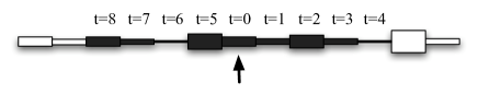
Figure 1: The figure represents the first eight time steps of IP dynamics in $d=1$. At each time step the throat of the growth interface with the maximal capillarity (i.e. minimal diameter) is occupied by the invader fluid. The throats have random capillarities, i.e. random diameters and, due to the extremal nature of the dynamics, its statistical properties do not depend on the PDF from which capillarities are extracted.

At $t=0$ the invader fluid is supposed to occupy only the central throat. At each time step the growth interface is given by the two non occupied throats in contact with the invaded region. The invaded region grows by occupying the interface throat with the maximal capillarity (i.e. minimal diameter). In this way the interface is updated by eliminating from it the selected throat and including the next one in the direction of growth. This is exactly equivalent to the task list problem for $p=1$ and $L=2$, with the set of the already executed tasks given by the invaded region, and the task list given by the two throats of interface. Analogously the case of the task list with $L>2$ can be mapped for $p=1$ into the case of IP on a star-like set of throats with $L$ linear branches GRC06 . For $0<p<1$ the task list problem would correspond to a sort of IP at finite temperature Ip1 which introduces a source of noise in the problem permitting random non extremal growths. The quantity $(1-p)$ is a measure of such thermal noise which vanishes for $p=1$ and becomes maximal for $p=0$.

In general for growth processes with quenched disorder it is very difficult to factorize the statistical weight of a growth path (i.e. selection sequence) into the product of probabilities of the composing elementary steps. The problem is that these single-step probabilities depend upon all the past history of the process, i.e, dynamics in quenched disorder present usually strong memory effects. This feature makes very difficult to evaluate the statistical weight of any possible history of the process which is usually the elementary ingredient to perform averages over the possible realizations of the dynamics. To overcome this difficulty, RTS gives a step-by-step procedure to write the exact evolution of the probabilities of the single steps conditional to the past history and the related conditional PDF of the random variables attached to the growing elements (“task priorities” in this case). Given two tasks with respective priorities $x$ and $y$, we call $\eta(x,y)$ the probability conditional to these values to execute the task with priority $x$. The form of $\eta$ is determined by the selection (i.e. growth in IP) rule of the model. Given the definition of the Barb́asi model and being $\theta(x)$ the Heaviside step function, we have:

$$\eta(x,y)=p\theta(x-y)+\frac{1-p}{2}\,.$$ (1)

If we now suppose that at the $t^{th}$ time-step of the selection dynamics the variables $x$ and $y$ are statistically independent and have respectively the PDFs conditional to the past history of the process $p(x,t)$ and $q(y,t)$, we can write the probability of selecting the task with priority $x$ conditional to the past history as

$$\mu(t)=\int_{0}^{1}\int_{0}^{1}dx\,dy\,p(x,t)q(y,t)\eta(x,y).$$ (2)

When the selection is done the selected task is removed from the list and replaced by a fresh new task with a random priority extracted from $\rho(x)$. The other task remains instead in the list. We indicate the first fresh task with $N$ (as “new”). The PDF of its priority conditional to the past history is simply $\rho(x)$ as it is new. The second task is consequently indicated with $O$ (as “old”), and we call the PDF of its priority, conditional to the past history of the task list, as $p_{O}(x,t)$. For all $t>0$ and $p>0$ it differs from $\rho(x)$. Given our particular form (1) of $\eta(x,y)$, $p_{O}(x,t)$ is, for $p>0$, more concentrated on the small values of $x$ than $\rho(x)$. At $t=0$ the initial condition is $p_{O}(x,0)=\rho(x)$. Since at each time-step the task $N$ is new, the priorities $x$ and $y$ of $N$ and $O$ are statistically independent and their joint probability factorizes into the product $\rho(x)p_{O}(y,t)$. Any realization of the task list (i.e. a selection path) lasting $\tau$ steps can be represented as a time ordered string of $\tau$ letters $N$ and $O$ (e.g. $NONNONO....$). In particular the statistical weight of the selection path $NN..N$ composed by $\tau$ subsequent events $N$ gives the probability that the waiting time of the task $O$, from the beginning of the list dynamics, is at least $\tau$. In terms of IP in $d=1$ this path represents a growth avalanche in one single direction starting at $t=0$ and lasting at least $\tau$ steps. We can rewrite Eq. (2) for both the cases in which the task $N$ or $O$ are selected at time $t$:

$$\left\{\begin{array}[]{l}\mu_{N}(t)=\int_{0}^{1}\int_{0}^{1}dx\,dy\,\rho(x)p_{O}(y,t)\eta(x,y)\\ \\ \mu_{0}(t)=1-\mu_{N}(t)=\int_{0}^{1}\int_{0}^{1}dx\,dy\,p_{O}(x,t)\rho(y)\eta(x,y)\end{array}\right.$$ (3)

For each of this two selection events we update consequently the conditional PDFs of the priorities including this last step in the past history conditioning probabilities. As explained above, the conditional PDF of the new task replacing the selected one is $\rho(x)$. Instead the conditional PDF $p_{O}(x,t+1)$ at time $t+1$ of the just unselected task, still in the list, is different in the two cases above. If the task $N$ is selected, the task $O$ remains $O$ also at the next time-step (see Fig.2). We can use the rules of the conditional probability to include the last selection step in the “memory” of the past history:

$$p_{O}(x,t+1)=\frac{1}{\mu_{N}(t)}p_{O}(x,t)\int_{0}^{1}dy\rho(y)\eta(y,x)\,.$$ (4)

If instead $O$ is selected at time $t$, it is removed, and the $N$ at time $t$ becomes the task $O$ at time $(t+1)$:

$$p_{O}(x,t+1)=\frac{1}{\mu_{O}(t)}\rho(x)\int_{0}^{1}dyp_{O}(y,t)\eta(y,x)\,.$$ (5)

The whole set of all possible selection paths can be represented as a non-Markovian binary branching process whose realizations tree is represented in Fig.2. The initial node (top vertex) represents the initial situation where one has two tasks with completely random priorities [i.e. distributed as $\rho(x)$]. From each node there is a bifurcation of possible choices: either task $N$ or $O$ is selected. Therefore each node of the tree represents the task list at the end of the time ordered selection path connecting directly the top vertex with the given node and is characterized by path-dependent conditional PDF $p_{O}$ and probabilities for the next bifurcation $\mu_{N}$ and $\mu_{O}$. The exact statistical weight of each path on the tree and the conditional PDF $p_{O}$ at the end of it can be calculated by applying the above RTS step-by-step procedure. Therefore the RTS provides a complete mathematical description of the task list dynamics. Note that the dynamics of the task list in this model is a binary branching process with memory, in the sense that the probabilities of a configuration at a given time depends for $p>0$ on all the past history of the list. This memory effect is maximized for $p=1$ when the list dynamics becomes deterministic and extremal.

A very important quantity in this class of dynamics is the average priority “histogram” Ip2 ; Ip1 , that is the statistical distribution of the priorities of the task list at a given time $t$ averaged over all the selection paths: $h(x,t)=[\rho(x)+\left<p_{O}(x,t)\right>_{t}]/2$. Hence, the evolution of $h(x,t)$ is directly given by that of $\rho_{1}(x,t)=\left<p_{O}(x,t)\right>_{t}$. The equation for its time evolution can be found by observing that at each binary branching starting from a node at time $t$ of the tree we can say that with probability $\mu_{N}(t)$ the priority conditional PDF $p_{O}(x,t)$ updates as in Eq. (4) and with probability $\mu_{O}(t)$ as in Eq. (5), i.e.

$$\pi_{O}(x,t+1;t) = p_{O}(x,t)\int_{0}^{1}dy\rho(y)\eta(y,x)$$

$$+ \rho(x)\int_{0}^{1}dyp_{O}(y,t)\eta(y,x)\,,$$

where $\pi_{O}(x,t+1;t)$ is the conditional PDF of the priority of the task $O$ at time $(t+1)$ conditional to the history only up to time $t$. By applying this average from the first time step it is simple to show that:

$$\rho_{1}(x,t+1) = \rho_{1}(x,t)\int_{0}^{1}dy\rho(y)\eta(y,x)$$ (6)

$$+ \rho(x)\int_{0}^{1}dy\rho_{1}(y,t)\eta(y,x)\,.$$

This is exactly the basic equation used in Vazquez05 to study the task list dynamics in the stationary state, i.e., when $\rho_{1}(x,t+1)=\rho_{1}(x,t)$. We show in the following that however in the limit $p\rightarrow 1$ the stationary state is reached only very slowly and that the waiting time distribution is determined by the finite time deviation from the stationary state at all time. This waiting time distribution is again a power law, but with a different exponent with respect to that found in Vazquez05 .

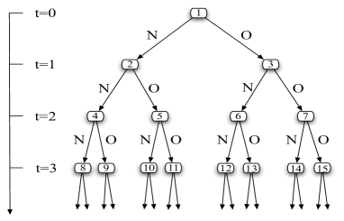
Figure 2: Tree representation of all the possible selection paths (i.e. realizations of the dynamics). At each time step either the fresh new task ($N$) either the old one ($O$) is selected. In general for $p>0$ $p_{O}(x,t)$ at the end of a path depend on the specific path. Only for $p=1$, when information on priorities and memory are maximal, $p_{O}(x,t)$ is the same for all paths.

We now solve exactly the RTS for the case $p=1$. For our calculation we use here $\rho(x)=1$ for $x\in[0,1]$ as in Vazquez05 because the path statistics, as aforementioned, does not depend on $\rho(x)$ for $p=1$. Hence Eqs. (3) above takes the simple form:

$$\left\{\begin{array}[]{l}\mu^{e}_{N}(t)=\int_{0}^{1}dx\,(1-x)p^{e}_{O}(x,t)\\ \\ \mu^{e}_{O}(t)=1-\mu^{e}_{N}(t)=\int_{0}^{1}dx\,xp^{e}_{O}(x,t)\,,\end{array}\right.$$

where the superscript “$e$” stands for “extremal”. Analogously Eqs. (4) and (5) for $p=1$ read respectively

$$p^{e}_{0}(x,t+1)=\frac{1}{\mu^{e}_{N}(t)}(1-x)p^{e}_{O}(x,t)$$

$$p^{e}_{0}(x,t+1)=\frac{1}{\mu^{e}_{O}(t)}\int_{x}^{1}dx\,p^{e}_{O}(x,t)\,.$$

using $p^{e}_{O}(x,0)=\rho(x)$ in the above equations, one finds that, for any selection path, $\mu_{N}^{e},\mu_{O}^{e}$ and $p^{e}_{O}$ becomes:

$$\mu_{N}^{e}(t)=\frac{t+1}{t+2}\;\;\;;\;\;\;\mu_{O}^{e}(t)=\frac{1}{t+2}$$ (7)

$$p^{e}_{O}(x,t)=(t+1)(1-x)^{t}\,.$$ (8)

Since $p^{e}_{O}(x,t)$ is independent of the considered path, $\rho_{1}(x,t)$ for $p=1$ coincides with it. Note that $\mu_{N}^{e}(t\!\!\rightarrow\!\!\infty)\rightarrow\!1$ and $\rho_{1}(x,t)=p^{e}_{O}(x,t\!\!\rightarrow\!\!\infty)\rightarrow\!\delta(x-0^{+})$ [where $\delta(x)$ is the Dirac delta function], i.e., in the infinite time limit the new fresh task is always selected as the old one has vanishing priority with probability one. The fact that both the $\mu^{e}$’s and the $p^{e}$’s at time $t$ are the same for each selection path of length $t$ is a feature of the $p=1$ case. This is not the case for $0<p<1$ where instead the conditional selection probability and priority PDFs at time $t$ depend on which specific selection path is considered. We now analyze the consequences of Eq. (7). It permits to find the waiting time distribution of a given task entered the list at time $t_{0}$. From Eq. (7) we find that for $p=1$ the waiting time is $\tau=0$ with probability $P(\tau=0;t_{0})=(t_{0}+1)/(t_{0}+2)$. The probability that it is still waiting after $\tau\geq 1$ steps, i.e. at time $t_{0}+\tau$, is:

$$W(\tau,t_{0})=\frac{1}{t_{0}+2}\prod_{t^{\prime}=1}^{\tau-1}\frac{t_{0}+t^{\prime}+1}{t_{0}+t^{\prime}+2}=\frac{1}{t_{0}+\tau+1}\,,$$

which is the probability of the path $ONN...N$ with one $O$ event at $t_{0}$ and $(\tau-1)$ subsequent $N$ events. Hence the probability that the waiting time is exactly $\tau\geq 1$ is

$$P(\tau;t_{0})=\frac{W(\tau;t_{0})}{t_{0}+\tau+2}=\frac{1}{(t_{0}+\tau+1)(t_{0}+\tau+2)}\,,$$ (9)

which is the statistical weight of the selection path $ONN...NO$ with one $O$ event at $t_{0}$, $(\tau-1)$ subsequent $N$ events and a final $O$ event. Note that this corresponds in IP to the statistical weight of an avalanche starting a time $t_{0}$ and lasting $\tau$ steps. The probability $P(\tau;t_{0})$ decreases as $\tau^{-2}$ for $\tau\gg t_{0}$ (a behavior confirmed by numerical simulations). Therefore the waiting time distribution for a task entered at time $t_{0}$ is normalizable in $\tau$, but with diverging mean value. This behavior is different from the power law $P(\tau)\sim\tau^{-1}$ found in Vazquez05 for the stationary state for $0<p<1$, which however disappears for $p\rightarrow 1^{-}$ as its amplitude vanishes in this limit. For the opposite limit $t_{0}\gg\tau\gg 1$ one can write $P(\tau;t_{0})\simeq t_{0}^{-2}(1-2\tau/t_{0})$, which decreases as $t_{0}^{-2}$ with $t_{0}$. This gives the rate of approach in the initial time $t_{0}$ to the trivial stationary state $P(\tau;t_{0}\rightarrow\infty)=1$ or $0$ respectively if $\tau=0$ or $\tau\geq 1$. This rate is very slow and there is no characteristic time after which one can say that the stationary state is attained in terms of $\tau$ dependence.

In order to study more in detail the approach to the stationary state for all $p$ and for $p\rightarrow 1$, we analyze Eq. (6) out of the stationary state. First of all we rewrite this equation using the explicit form (1) of $\eta(x,y)$ for this model and $\rho(x)=1$ for $x\in[0,1]$:

$$\rho_{1}(x,t+1) = \rho_{1}(x,t)\left[p(1-x)+\frac{1-p}{2}\right]$$ (10)

$$+ p\int_{x}^{1}dy\rho_{1}(y,t)+\frac{1-p}{2}\,.$$

We now put $\rho_{1}(x,t)=\rho_{1}^{(s)}(x)+\delta\rho_{1}(x,t)\,,$ where $\rho_{1}^{(s)}(x)$ is the stationary solution found in Eq. (4) of Vazquez05 :

$$\rho_{1}^{(s)}(x)=\frac{1+p}{1-p}\frac{1}{[1+\frac{2p}{1-p}x]^{2}}$$ (11)

and $\delta\rho_{1}(x,t)$ is the finite time deviation from it. For $p\rightarrow 1$ the PDF $\rho_{1}^{(s)}(x)\rightarrow\delta(x-0^{+})$ and it coincides with Eq. (8) for $t\rightarrow\infty$. Since $\rho_{1}(x,t)$ and $\rho_{1}^{(s)}(x)$ are both normalized to unity, we have $\int_{0}^{1}dx\delta\rho_{1}(x,t)=0$. Therefore as a first order approximation we put $\int_{x}^{1}dy\,\delta\rho_{1}(y,t)\simeq-x\delta\rho_{1}(x,t)$. Taking also the continuous time approximation $[\delta\rho_{1}(x,t+1)-\delta\rho_{1}(x,t)]\simeq d\delta\rho_{1}(x,t)/dt$, we can rewrite Eq. (10) in terms of $\delta\rho_{1}(x,t)$ as

$$\frac{d\delta\rho_{1}(x,t)}{dt}\simeq-\left(\frac{1-p}{2}+2px\right)\delta\rho_{1}(x,t)\,.$$ (12)

Hence $\delta\rho_{1}(x,t)$ decays exponentially in time with an $x-$dependent time constant inversely proportional to $[(1-p)/2+2px]$. For $p<1$, at each $x$ the perturbation decays exponentially fast and the stationary state is attained, while for $p\rightarrow 1$ the time constants becomes proportional to $1/x$ and the perturbation in the region around $x=0$ relaxes very slowly. But from Eq. (11) it is exactly in this region that for $p\rightarrow 1$ all the measure $\rho^{(s)}(x)$ is concentrated. This confirms our previous conclusion that for $p\rightarrow 1$ the stationary state is very slowly attained and finite time deviation from it play a fundamental role in determining the rate of decrease of the waiting time distribution.

In this paper we have studied an interesting queueing model of task list dynamics introduced by Barábasi. Through a statistical method called RTS, we are able to give a complete probabilistic description of the dynamics even out of stationarity. We find that for $0<p<1$ finite time deviations from stationarity relaxes exponentially fast and, consequently, the dynamics is well described by the stationary state. However for $p\rightarrow 1$ the stationary state becomes trivial and finite time deviations relaxes so slowly that the task list dynamics has to be described as an intrinsically non stationary dynamics. This is characterized by power law waiting time distributions with a characteristic exponent which is different from the one found Vazquez05 in the stationary state for $0<p<1$.

GC acknowledges support from EU Project DELIS

References

- (1) HC Tijms, A First Course in Stochastic Models, Wiley Chichester, (2003).
- (2) L. Breuer and D. Baum An Introduction to Queueing Theory and Matrix-Analytic Methods. Springer Verlag (2005).
- (3) A.-L. Barabási, Nature (London) 207, 435 (2005).
- (4) A. Vázquez, J. G. Oliveira, Z. Dezső, K.-I. Goh, I. Kondor, A.-L. Barabási Physical Review E 73, 036127 (2006).
- (5) A. Vazquez, Physical Review Letters 95, 248701 (2005).
- (6) M. Marsili, Journal of Statistical Physics, 77 733–754,(1994); A. Gabrielli, M. Marsili, R. Cafiero, L. Pietronero, Journal of Statistical Physics, 84 889–893, (1996).
- (7) D. Wilkinson and J.F. Willemsen, Journal of Physics A, 16, 3365-3376 (1983).
- (8) A. Gabrielli, R. Cafiero, M. Marsili, and L. Pietronero, Phys. Rev. E, 54, 1406 (1996).
- (9) M. Felici, G. Caldarelli, A. Gabrielli, and L. Pietronero, Phys. Rev. Lett., 86, 1896 (2001).
- (10) A. Gabrielli, F. Rao, G. Caldarelli, in preparation.
- (11) A. Gabrielli, G. Caldarelli, L. Pietronero, Physical Review E 62, 7638–7641 (2000)