Inverse cascades and $\alpha$-effect at low magnetic Prandtl number

Abstract

Dynamo action in a fully helical Beltrami (ABC) flow is studied using both direct numerical simulations and subgrid modeling. Sufficient scale separation is given in order to allow for large-scale magnetic energy build-up. Growth of magnetic energy obtains down to a magnetic Prandtl number $P_{M}=R_{M}/R_{V}$ close to $0.005$, where $R_{V}$ and $R_{M}$ are the kinetic and magnetic Reynolds numbers. The critical magnetic Reynolds number for dynamo action $R_{M}^{c}$ seems to saturate at values close to $20$. Detailed studies of the dependence of the amplitude of the saturated magnetic energy with $P_{M}$ are presented. In order to decrease $P_{M}$, numerical experiments are conducted with either $R_{V}$ or $R_{M}$ kept constant. In the former case, the ratio of magnetic to kinetic energy saturates to a value slightly below unity as $P_{M}$ decreases. Examination of energy spectra and structures in real space both reveal that quenching of the velocity by the large-scale magnetic field takes place, with an inverse cascade of magnetic helicity and a force-free field at large scale in the saturated regime.

I INTRODUCTION

In recent years the increase in computing power, as well as the development of subgrid models for magnetohydrodynamic (MHD) turbulence Müller and Carati (2002a, b); Ponty et al. (2004); Mininni et al. (2005a, b) has allowed the study of a numerically almost unexplored territory: the regime of low magnetic Prandtl number ($P_{M}=R_{M}/R_{V}$, where $R_{V}$ and $R_{M}$ are respectively the kinetic and magnetic Reynolds numbers). This MHD regime is of particular importance since several astrophysical Parker (1979) and geophysical Roberts and Glatzmaier (2001); Kono and Roberts (2002) problems are characterized by $P_{M}<1$, as for example in the liquid core of planets such as Earth, or in the convection zone of solar-type stars. Also, liquid metals (e.g., mercury, sodium, or gallium) used in the laboratory in attempting to generate dynamo magnetic fields are in this regime Noguchi et al. (2002); Pétrélis et al. (2003); Sisan et al. (2003); Spence et al. (2006).

In recent publications Schekochihin et al. (2004); Ponty et al. (2005); Schekochihin et al. (2005); Mininni et al. (2005c); Mininni and Montgomery (2005), driven turbulent MHD dynamos were studied numerically, within the framework of rectangular periodic boundary conditions. As $P_{M}$ is lowered at fixed viscosity the magnetofluid becomes more resistive than it is viscous, and it was found that magnetic fields were harder to excite by the dynamo process because of the increased turbulence in the fluid. The principal result was in obtaining the dependence of the critical magnetic Reynolds number $R_{M}^{c}$ with the magnetic Prandtl number. These studies were done for several settings, ranging from coherent helical Mininni and Montgomery (2005) and non-helical Ponty et al. (2005); Mininni et al. (2005c) forcing, as well as for random forcing Schekochihin et al. (2004, 2005). While for coherent forcing an asymptotic regime was found at small values of $P_{M}$, the behavior of $R_{M}^{c}$ for random forcing is still unclear (see also Vincenzi (2002); Boldyrev and Cattaneo (2004) for theoretical arguments based on the Kazantsev model Kazanstev (1968)).

For coherent forcing such as the Taylor-Green vortex (that corresponds to several laboratory experiments using two counter-rotating disks), the value of $R_{M}^{c}$ was observed to increase by a factor larger than six before the asymptotic regime for small values of $P_{M}$ was reached Ponty et al. (2005). Although the precise value of $R_{M}^{c}$ in experiments is expected to be modified by the presence of boundaries, it is of interest to study what properties of the forcing can modify and decrease its value. It is well known from theory Moffatt (1978), two-point closure models Pouquet et al. (1976), and direct numerical simulations (DNS) at $P_{M}=1$ Meneguzzi et al. (1981); Gilbert et al. (1988); Brandenburg (2001) that the presence of net helicity in the flow helps the dynamo and decreases the value of $R_{M}^{c}$.

In Mininni and Montgomery (2005) dynamos with a helical forcing function were studied using the Roberts flow, but mechanical energy was injected at a wavenumber $|{\bf k}|=\sqrt{2}$, which left little room in the spectrum for any back-transfer of magnetic helicity as expected in the helical case Steenbeck et al. (1966); Pouquet et al. (1976); Krause and Rädler (1980); indeed, $|{\bf k}|=1$ is the only possibility since the computations are done in a box of length $2\pi$ corresponding to a $k=1$ gravest mode. In this work, in contrast, we study the effect of a fully helical Arn’old-Childress-Beltrami (ABC) forcing Childress and Gilbert (1995) with energy injected at a slightly smaller scale (note that the ABC forcing is related to the Roberts forcing, since it can be defined as a superposition of three Roberts flows). As a result of the intermediate scale forcing, some $\alpha$-effect or inverse cascade of magnetic helicity can a priori develop and a magnetic field at large scales can grow.

ABC flows and helical dynamos were explored in many different contexts in the literature (see e.g. Galanti et al. (1992) for a study close to $P_{M}=1$, and Ponty et al. (1995); Hollerbach et al. (1995) for studies in the context of fast dynamo action). The main aim of the present work is to study the impact of helical flows at intermediate scales in the development of magnetic fields through dynamo action at $P_{M}<1$. In this context, it is worth noting that some simulations of ABC dynamos in the low magnetic Prandtl number regime were discussed in Refs. Brandenburg (2001); Archontis et al. (2003), although no systematic exploration of the space of parameters was attempted. Also, Ref. Mininni (2006) presented some preliminary results for the kinematic dynamo regime with ABC forcing. In this work we will focus on the study of the generation of large scale magnetic fields and of the non-linear saturation regime. A similar study was recently conducted in Ref. Frick et al. (2006) using mean field theory Steenbeck et al. (1966); Krause and Rädler (1980) and shell models. To the best of our knowledge, ours is the first attempt to systematically study the saturation values of the fields for helical flows at $P_{M}<1$ in numerical simulations.

II DEFINITIONS AND METHODOLOGY

In a familiar set of dimensionless (“Alfvénic”) units the equations of magnetohydrodynamics are:

$$\frac{\partial{\bf v}}{\partial t}+{\bf v\cdot\nabla v} = -{\bf\nabla}{\mathcal{P}}+{\bf j\times B}+\nu\nabla^{2}{\bf v}+{\bf f},$$ (1)

$$\frac{\partial{\bf B}}{\partial t}+{\bf v\cdot\nabla B} = {\bf B\cdot\nabla v}+\eta\nabla^{2}{\bf B},$$ (2)

with ${\bf\nabla\cdot v}={\bf\nabla\cdot B}=0$. Here, ${\bf v}$ is the velocity field, regarded as incompressible, and ${\bf B}$ is the magnetic field, related to the electric current density ${\bf j}$ by ${\bf j}={\bf\nabla\times B}$. ${\mathcal{P}}$ is the pressure, obtained by solving the Poisson equation that results from taking the divergence of Eq. (1) and using the incompressibility condition ${\bf\nabla\cdot v}=0$. The viscosity $\nu$ and magnetic diffusivity $\eta$ define mechanical Reynolds numbers and magnetic Reynolds numbers respectively as $R_{V}=LU/\nu$ and $R_{M}=LU/\eta$. Here $U$ is a typical turbulent flow speed (the r.m.s. velocity in the following sections, $U=\left<u^{2}\right>^{1/2}$, with the brackets denoting spatial averaging), and $L$ is a length scale associated with spatial variations of the large-scale flow (the integral length scale of the flow). We can also define a Taylor based Reynolds number $R_{\lambda}=\lambda U/\nu$, where $\lambda$ is the Taylor lengthscale, defined below.

Some global quantities will appear repeatedly in the next sections. These are the total energy (the sum of the kinetic $E_{V}$ and magnetic $E_{M}$ energies) $E=E_{V}+E_{M}={{1}\over{2}}\int({\bf u}^{2}+{\bf B}^{2})\,dV$, the magnetic helicity $H_{M}=\int{\bf A}\cdot{\bf B}\,dV$ (where ${\bf A}$ is the vector potential, defined such as ${\bf B}=\nabla\times{\bf A}$), and the kinetic helicity $H_{V}=\int{\bf v}\cdot\mbox{\boldmath$\omega$}\,dV$ (where $\mbox{\boldmath$\omega$}=\nabla\times{\bf v}$ is the vorticity). While $E$ and $H_{M}$ are ideal ($\nu=\eta=0$) quadratic invariants of the MHD equations, $H_{K}$ is not. In practice, kinetic helicity in helical dynamos is injected into the flow by the mechanical forcing ${\bf f}$ (e.g., by rotation and stratification in geophysical and astrophysical flows Moffatt (1978)).

Equations (1) and (2) are solved numerically using a parallel pseudospectral code, as described in Refs. Mininni et al. (2005c); Mininni and Montgomery (2005). We impose rectangular periodic boundary conditions throughout, using a three-dimensional box of edge $2\pi$. The integral and Taylor scales are defined respectively as

$$L=2\pi\sum_{\bf k}{k^{-1}|\hat{\bf v}({\bf k})|^{2}}\bigg{/}\sum_{\bf k}{|\hat{\bf v}({\bf k})|^{2}},$$ (3)

$$\lambda=2\pi\left(\sum_{\bf k}{|\hat{\bf v}({\bf k})|^{2}}\bigg{/}\sum_{\bf k}{k^{2}|\hat{\bf v}({\bf k})|^{2}}\right)^{1/2},$$ (4)

where $\hat{\bf v}({\bf k})$ is the amplitude of the mode with wave vector ${\bf k}$ ($k=|{\bf k}|$) in the Fourier transform of ${\bf v}$.

The external forcing function ${\bf f}$ in Eq. (1) injects both kinetic energy and kinetic helicity. For ${\bf f}$ we use the ABC flow

$${\bf f}_{\rm ABC} = f_{0}\left\{\left[B\cos(k_{F}y)+C\sin(k_{F}z)\right]\hat{x}+\right.{}$$ (5)

$${}+\left[A\sin(k_{F}x)+C\cos(k_{F}z)\right]\hat{y}+{}$$

$${}+\left.\left[A\cos(k_{F}x)+B\sin(k_{F}y)\right]\hat{z}\right\},$$

with $A=0.9$, $B=1$, $C=1.1$ Archontis et al. (2003), and $k_{F}=3$. The ABC flow is an eigenfunction of the curl with eigenvalue $k_{F}$, and as a result if used as an initial condition it is an exact solution of the Euler equations. In the hydrodynamic simulations, for large enough $\nu$ (small $R_{V}$) the laminar solution is stable. As $\nu$ is decreased the laminar flow becomes unstable and develops turbulence (see Podvigina and Pouquet (1994) for a study of the early bifurcations at intermediate Reynolds numbers).

To properly resolve the turbulent flow, the maximum wavenumber in the code $k_{max}=N/3$ ($N$ is the linear resolution and the standard $2/3$-rule for dealiasing is used) has to be smaller than the mechanic dissipation wavenumber $k_{\nu}=(\epsilon/\nu^{3})^{1/4}$ ($\epsilon\sim U^{3}/L$ is the energy injection rate). As a result, as $\nu$ decreases and $R_{V}$ increases, the linear resolution $N$ has to be increased. At some point the use of DNS to solve Eqs. (1) and (2) turns to be too expensive from the computational point of view and some kind of model for unresolved scales is needed.

To extend the range of $R_{V}$ and $P_{M}$ studied, we use the Lagrangian average MHD equations (LAMHD, also known as the MHD $\alpha$-model) Holm (2002a, b); Mininni et al. (2005a)

$$\frac{\partial{\bf v}}{\partial t}+{\bf u}_{s}\cdot\nabla{\bf v} = -v_{j}\nabla u_{s}^{j}-\nabla\widetilde{{\cal P}}+{\bf j}\times{\bf B}_{s}$$ (6)

$$+\nu\nabla^{2}{\bf v}+{\bf f},$$

$$\frac{\partial{\bf B}_{s}}{\partial t}+{\bf u}_{s}\cdot\nabla{\bf B}_{s} = {\bf B}_{s}\cdot\nabla{\bf u}_{s}+\eta\nabla^{2}{\bf B}.$$ (7)

In these equations, the pressure $\widetilde{{\cal P}}$ is determined, as before, from the divergence of Eq. (6) and the incompressibility condition. The subindex $s$ denotes smoothed fields, related to the unsmoothed fields by

$${\bf v} = \left(1-\alpha_{V}^{2}\nabla^{2}\right){\bf u}_{s}$$ (8)

$${\bf B} = \left(1-\alpha_{B}^{2}\nabla^{2}\right){\bf B}_{s}.$$ (9)

The total energy in this system is given by $E=E_{V}+E_{M}={{1}\over{2}}\int({\bf v}\cdot{\bf u}_{s}+{\bf B}\cdot{\bf B}_{s})\,dV$; it is one of the ideal quadratic invariants of the LAMHD equations. Equivalently, the magnetic helicity invariant is now given by $H_{M}=\int{\bf A}_{s}\cdot{\bf B}_{s}dV$, where the smooth vector potential is defined such as ${\bf B}_{s}=\nabla\times{\bf A}_{s}$. The expression for the kinetic helicity is the same in MHD and LAMHD.

The LAMHD equations are a regularization of the MHD equations, and as a result they allow for simulations of turbulent flows at a given Reynolds number using a lower resolution than in DNS. This subgrid model was validated against DNS of MHD flows in Mininni et al. (2005a, b). As in previous studies of dynamo action at low $P_{M}$, the ratio of the two filtering scales $\alpha_{V}$ and $\alpha_{B}$ was set using the ratio of the kinetic and magnetic dissipation scales, i.e. $\alpha_{V}/\alpha_{B}=P_{M}^{3/4}$ Ponty et al. (2005). The value of $\alpha_{V}$ depends on the linear resolution and was adjusted to $1/\alpha_{V}\approx k_{max}/2$ Geurts and Holm (2006).

Table 1: Parameters for the simulations: kinematic viscosity $\nu$, Taylor Reynolds number $R_{\lambda}$, mechanical Reynolds number $R_{V}$, range of values of the magnetic Reynolds number $R_{M}$ for a given flow, linear resolution $N$, and value of the mechanic filter length $\alpha_{V}$ (with $\alpha_{V}/\alpha_{B}=[R_{M}/R_{V}]^{3/4}$ in each case). For direct simulations (no subgrid model), $\alpha_{V}$ need not be defined. Runs in set 6a have the same values of parameters than in set 6, but a subgrid model at a lower resolution was used. Run 9 has the same parameters as set 9b with $R_{M}=41$ but was done using a DNS. The lowest $P_{M}$ achieved for this set of runs is $\approx 0.005$.

Set	$\nu$	$R_{\lambda}$	$R_{V}$	$R_{M}$	$N$	$\alpha_{V}$
1	$0.2$	11	11	9–16	64	-
2	$0.1$	21	23	10–19	64	-
3	$4\times 10^{-2}$	55	71	17–71	64	-
4	$9\times 10^{-3}$	161	240	18–54	64	-
5	$4\times 10^{-3}$	250	450	15–450	128	-
6	$2\times 10^{-3}$	360	820	10–41	256	-
6a	$2\times 10^{-3}$	290	840	10–41	64	$0.1$
7	$1\times 10^{-3}$	340	1700	14–42	128	$0.0625$
8	$6.2\times 10^{-4}$	680	2500	39	512	-
9	$5\times 10^{-4}$	500	3400	41	512	-
9b	$5\times 10^{-4}$	500	3400	14–42	256	$0.03125$
10	$2.5\times 10^{-4}$	1100	6200	77	1024	-

In the next section, we describe the computations and the results for both the kinematic dynamo regime [where ${\bf j\times B}$ is negligible in Eq. (1)], and for full MHD (where the Lorentz force modifies the flow). The first step is to establish what are the thresholds in $R_{M}$ at which dynamo behavior sets in as $R_{V}$ is raised and $P_{M}$ is decreased (Section III.1). The procedure to do this is the following (see e.g., Ref. Ponty et al. (2005)). First a hydrodynamic simulation at a given value of $R_{V}$ is done. Then, a small and random (non-helical) magnetic field is introduced, and several simulations are done changing only the value of $R_{M}$. At a given $R_{M}$, the magnetic energy can either decay or grow exponentially. In each simulation, the growth rate $\sigma$ is then defined as $\sigma=d\ln(E_{M})/dt$. The critical magnetic Reynolds number $R_{M}^{c}$ for the onset of dynamo action corresponds to $\sigma=0$, and in practice is obtained from a linear interpolation between the two points with respectively positive and negative $\sigma$ closest to zero. The growth rate $\sigma$ is typically expressed in units of the reciprocal of the large-scale eddy turnover time $T=L/U$.

Figure 1: Critical magnetic Reynolds $R_{M}^{c}$ as a function of $P_{M}^{-1}$: DNS (solid line) and LAMHD (dotted line). Note the saturation for $P_{M}\leq 0.02$.

Once the values of $R_{M}^{c}$ for different values of $P_{M}\leq 1$ have been found, simulations for $R_{M}>R_{M}^{c}$ are conducted for longer times (Section III.2). In this case, magnetic fields are initially amplified exponentially, and then saturate due to the back reaction of the magnetic field on the flow. In helical flows, this saturation is accompanied by the growth of magnetic fields in the largest scale available in the box. In this regime, we will study the maximum value attained by the magnetic energy as a function of $P_{M}$ (Section III.3), as well as the amount of magnetic energy at scales larger than the forcing scale (Section III.4). Finally, Section 4 is the conclusion.

Figure 2: Growth rates as a function of $R_{M}$. Each line corresponds to several simulations at constant $R_{V}$ (fixed $\nu$), and each point in the line indicates the exponential growth (or decay) rate at a fixed value of $R_{M}$. The point where each curve crosses $\sigma=0$ gives the threshold $R_{M}^{c}$ for dynamo instability. Points from DNS are connected with solid lines, and labels are: set 1 ($\times$), set 2 ($\square$), set 3 ($\bigtriangleup$), set 4 ($\diamond$), set 5 ($*$), and set 6 ($+$). Points from LAMHD simulations are connected with dotted lines: set 6a ($+$), set 7 ($\times$), and set 9b ($\square$). Note the accumulation of lines near $R_{M}\approx 20$.

III SIMULATIONS AND RESULTS

In order to obtain a systematic study of dynamo action for ABC forcing and $P_{M}\leq 1$, a suite of several simulations was conducted. Table 1 shows the parameters used in the simulations. Note that when a range is invoked in the values of $R_{M}$, it indicates several runs were done with the same value of $R_{V}$ but changing the value of $R_{M}$ to span the range (typically three to five runs). The set of runs 6 and 6a have the same parameters ($\nu$, $\eta$, and r.m.s velocity), but while set 6 comprises DNS at resolutions of $256^{3}$ grid points, in set 6a the spatial resolution is $64^{3}$ and the LAMHD equations were used in order to further the testing of the model. Similar considerations apply to run 9 and set 9b.

III.1 Threshold for dynamo action

Figure 3: Time history of the magnetic energy for runs in set 6 (dashed line) and in set 6a (solid line) with $R_{M}\approx 41$ and $P_{M}=5\times 10^{-2}$. The inset shows the time evolution of the magnetic energy after the nonlinear saturation, in linear scale.

Figure 1 summarizes the results of the study of the dependence of the threshold $R_{M}^{c}$ as $P_{M}$ is decreased. For values of $R_{M}$ above the curve, dynamo action takes place and initially small magnetic fields are amplified. Below the curve, Ohmic dissipation is too large to sustain a dynamo. Noteworthy is the qualitative similarity of the curve between the ABC flow and previous results using different mechanical forcings Ponty et al. (2005); Mininni et al. (2005c); Mininni and Montgomery (2005). Namely, an increase in $R_{M}^{c}$ is observed as turbulence develops, and then an asymptotic regime is found in which the value of $R_{M}^{c}$ is independent of $P_{M}$. Note that LAMHD simulations were used to extend the study for values of $P_{M}$ smaller than what can be studied using DNS. Simulations at the same value of $P_{M}$ were carried with the two methods to validate the results from the subgrid model (sets 6 and 6a). This procedure was used before in Ref. Ponty et al. (2005). As in the previous study, the LAMHD equations slightly overestimate the value of $R_{M}^{c}$.

Figure 4: Time history of the magnetic energy for runs in set 5 (constant $R_{V}\approx 450$). The magnetic Reynolds number in each run is $R_{M}\approx 22$ (dashed line), $R_{M}\approx 45$ (dash-dotted line), $R_{M}\approx 180$ (dotted line), and $R_{M}\approx 450$ (solid line).

Besides the similarities in the shape of the curves for different forcing functions, two quantitative differences are striking: (i) only a mild rise in $R_{M}^{c}$ is observed here as $P_{M}$ is decreased (a factor 2, while a factor larger than 6 obtains for the Taylor-Green vortex Ponty et al. (2005)); and (ii) the asymptotic value of $R_{M}^{c}$ for small values of $P_{M}$ is ten times smaller than for other flows studied Ponty et al. (2005); Mininni and Montgomery (2005). A similar result was obtained using mean field theory and shell models in Ref. Frick et al. (2006), and the quantitative differences observed were associated with the relative ease to excite large-scale helical dynamos compared with non-helical and small-scale dynamos.

Note that the curve in Fig. 1 was constructed using the sets 1 to 7 and 9b of Table 1. Several runs at constant $R_{V}$ but varying $R_{M}$ are required to define $R_{M}^{c}$. Set 9b reveals a dynamo at the lowest magnetic Prandtl number known today in numerical simulations, namely $P_{M}=4.7\times 10^{-3}$.

Figure 5: Time history of (minus) the magnetic helicity for runs in set 5 (constant $R_{V}\approx 450$). The magnetic Reynolds number in each run is $R_{M}\approx 22$ (dashed line), $R_{M}\approx 45$ (dash-dotted line), $R_{M}\approx 180$ (dotted line), and $R_{M}\approx 450$ (solid line).

Figure 2 shows the details of how the thresholds for the determination of the $R_{M}^{c}=f(P_{M}^{-1})$ curve were calculated. For small initial $E_{M}$, broadly distributed over a set of wavenumbers, $\eta$ was decreased in steps to raise $R_{M}$ in the same mechanical setting until a value of $\sigma\approx 0$ was identified. A linear fit between the two points with $\sigma$ closest to $0^{\pm}$ provides a single point on the curves in Fig. 1. Note that Figure 2 also gives bounds for the uncertainties in the determination of the threshold $R_{M}^{c}$ (see e.g. Ref. Ponty et al. (2005)): errors in Fig. 1 can be defined as the distance between the value of $R_{M}^{c}$ and the value of $R_{M}$ in the simulation with $\sigma$ closest to 0. Note also the asymptotic approach to a growth rate of order unity for large values of the magnetic Reynolds number, as for example in the runs in set 5.

III.2 Time evolution

A comparison of the time evolution of the magnetic energy in two dynamo runs with the same mechanic and magnetic Prandtl number ($R_{M}\approx 41$, $P_{M}=5\times 10^{-2}$) is shown in Fig. 3. One of the runs is a DNS from set 6, while the other is a LAMHD simulation from set 6a. Two different stages can be identified at first sight in these runs. The kinematic regime at early times, with an exponential amplification of the magnetic energy (used to define the growth rates and thresholds in Figs. 1 and 2), and the nonlinear saturated regime at late times. As expected from the results discussed in the previous subsection, the LAMHD equations at a coarser grid ($64^{3}$) are able to capture the kinematic dynamo regime. While in the DNS with a resolution of $256^{3}$ the growth rate is $\sigma\approx 0.18$, in the LAMHD simulation $\sigma\approx 0.20$. But the LAMHD simulation also captures properly the nonlinear saturation (albeit the saturated level is reached a bit earlier) and the amplitudes of the magnetic energy in the steady state are comparable (see insert in Fig. 3). Small differences observed in the time evolution are likely due to differences in the initial random magnetic seed. In the following, we shall use both DNS and LAMHD simulations to study the nonlinear saturated regime at low $P_{M}$.

Figure 6: Time history of the magnetic energy in simulations at constant $R_{M}\approx 41$ ($\eta=4\times 10^{-2}$). The different runs are taken from set 3 ($P_{M}=1$, dash), set 4 ($P_{M}=0.225$, dot), set 5 ($P_{M}=0.1$, dash-dot), set 6 ($P_{M}=0.05$, solid), set 7 ($P_{M}=0.025$, dash-triple dot), and finally set 9 ($P_{M}=0.0125$, long dash).

In helical flows, as magnetic energy saturates, a large scale magnetic field develops (i.e., at scales larger than the forcing scale) due to the helical $\alpha$-effect Steenbeck et al. (1966); Pouquet et al. (1976); Moffatt (1978); Krause and Rädler (1980); Brandenburg (2001); Brandenburg and Subramanian (2005). It is of interest to know what happens with the amplitude of the magnetic field as the value of $P_{M}$ is decreased. An example is shown in Figure 4, which gives the magnetic energy as a function of time for runs in set 5. Only the value of $R_{M}$ (and therefore of $P_{M}$) is changed between the runs ($R_{V}\approx 450$ in all runs and $P_{M}$ varying from 1 to $0.03$). For large values of $R_{M}$ (but not necessarily for values of $P_{M}$ close to unity), the growth rate $\sigma$ is independent of $R_{M}$ and of order one as noted in Section III.1. Furthermore, as $P_{M}$ is decreased, both $\sigma$ and the saturation value of the magnetic energy decrease. However, for the lowest value of $P_{M}$, the magnetic Reynolds number is quite low and in that context computations at a higher value of $R_{V}$ and with the same sets of $P_{M}$ are of value to see what fraction of the present result is a threshold effect at low $R_{M}$.

Figure 7: Saturation value of the magnetic energy (normalized by the kinetic energy in the saturated regime). The triangles correspond to simulations at constant $R_{V}$, while the squares correspond to simulations at constant $R_{M}$ (squares connected with solid lines are from DNS, while squares connected with dotted lines are from LAMHD simulations). Note the saturation at low $P_{M}$ for constant $R_{M}$ runs.

Figure 5 shows the evolution of the magnetic helicity as a function of time for the same simulations than in Fig. 4. The external forcing injects positive kinetic helicity in the flow. In the kinematic regime, the $\alpha$ effect is proportional to minus the kinetic helicity Steenbeck et al. (1966); Krause and Rädler (1980). From mean field theory, the magnetic field in the large scales should grow with magnetic helicity of the same sign than the $\alpha$ effect (negative), as indeed observed (see Refs. Brandenburg (2001); Mininni et al. (2003) for helical dynamo simulations at $P_{M}=1$). In the simulations, magnetic helicity grows exponentially during the kinematic regime. In runs with small $R_{M}$, the saturated state is reached shortly after the saturation of the exponential phase. But as $R_{M}$ is increased, it is now clear that an intermediate stage develops in which magnetic energy and helicity keep growing slowly. As a result, saturation takes place in longer times, and the time to reach the final steady state depends on the large scale magnetic diffusion time ($T_{\eta}\approx 4\pi^{2}/\eta$). The dependence of the saturation time with $R_{M}$ can be observed in Fig. 5. It is also worth mentioning that even in the runs with $P_{M}<1$, the saturation of magnetic helicity can be well described by the formula $H_{M}(t)\sim 1-\exp[-2\eta k_{0}^{2}(t-t_{\rm sat})]$, where $k_{0}=1$ is the gravest mode, and $t_{\rm sat}$ is the saturation time of the small scale magnetic field Brandenburg (2001). This indicates that the slow saturation of the dynamo is dominated by the evolution of the magnetic helicity in the largest scale in the system.

Figure 8: Saturation value of the magnetic dissipation rate normalized by the kinetic energy in the saturated regime. The triangles correspond to simulations at constant $R_{V}$, while the squares correspond to simulations at constant $R_{M}$ (squares connected with solid lines are from DNS, while squares connected with dotted lines are from LAMHD simulations).

From Figs. 4 and 5 it seems apparent that small values of $P_{M}$ have a negative impact on the amplitude of the magnetic field generated by the dynamo. However, different results are obtained when the space of parameters is explored keeping $R_{M}$ constant and increasing $R_{V}$, as another way to decrease $P_{M}$. Figure 6 shows the results in this case for the time evolution of the magnetic energy. As $R_{V}$ is increased from small values, a drop in the growth rate $\sigma$ and in the saturation value of the magnetic energy is observed. But then an asymptotic regime is reached, in which both $\sigma$ and the saturation value seem to be roughly independent of $R_{V}$ and $P_{M}$. As a result, we conclude that the behavior observed in Figs. 4 and 5 is the result of critical slowing down: if the space of parameters is explored at constant $R_{V}$, as $P_{M}$ is decreased $R_{M}$ gets closer to $R_{M}^{c}$ until no dynamo action is possible. On the other hand, all the simulations with $P_{M}\leq 0.05$ shown in Fig. 5 have $R_{M}/R_{M}^{c}$ approximately constant (see Fig. 1) and critical slowing down is not observed. However, we note that the value of $R_{M}$ for these runs is still modest.

III.3 Saturation values

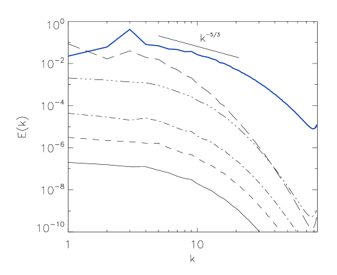
Figure 9: (Color online) Kinetic energy spectrum at $t=0$ [thick (blue) lines], and magnetic energy spectrum (thin lines) at different times: $t=11$ (solid line), $t=29$ (dashed line), $t=47$ (dash-dotted line), $t=95$ (dash-triple dotted line), $t=120$ (long dashed line). The spectra are for a run in set 6 with $R_{M}\approx 41$. The last time is in the saturation regime (see Fig. 6).

The amplitude of the magnetic energy (normalized by the kinetic energy), after the nonlinear saturation takes place, as a function of the magnetic Prandtl number is shown in Fig. 7. This figure summarizes the results discussed in Figs. 4 and 6. As the value of $P_{M}$ is decreased, if $R_{V}$ is kept constant and $R_{M}$ (and thus $P_{M}$) decreases, the saturation of the dynamo takes place for lower values of the magnetic energy. This is to be expected since as we decrease $P_{M}$ we also decrease $R_{M}$ and at some point $R_{M}^{c}$ is reached. It is not clear whether such a strong dependence would be observed if the constant $R_{V}$ runs were performed at substantially higher values of $R_{V}$ as found in astronomical bodies and in the laboratory; however, such runs would be quite demanding from a numerical standpoint unless one resorts to LES (Large Eddy Simulations) techniques, few of which have been developed in MHD (see e.g., Müller and Carati (2002a, b); Ponty et al. (2004)). For values of $R_{M}$ smaller than $R_{M}^{c}$, no dynamo action is expected and the ratio $E_{M}/E_{V}$ should indeed go to zero. On the other hand, in the simulations with constant $R_{V}$, the ratio $E_{M}/E_{V}$ seems to saturate for $P\lesssim 0.25$ and reach an approximately constant value close to $\approx 0.5$. This indicates that small scale turbulent fluctuations in the velocity field are strongly quenched by the large scale magnetic field, as will be also shown later in the spectral evolution of the energies. The ratio $E_{M}/E_{V}$ in helical large-scale dynamos is also expected to be dependent on the scale separation between the forcing wavenumber (here fixed to $k_{F}=3$) and the largest wavenumber in the system (here $k=1$). As the scale separation increases and there is more space for an inverse cascade of magnetic helicity, we expect the ratio $E_{M}/E_{V}$ in the $P_{M}<1$ regime to also increase.

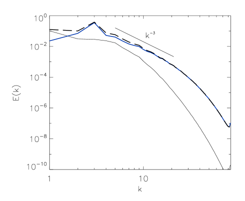
Figure 10: (Color online) Kinetic [thick (blue) line] and magnetic energy spectra (thin line) at $t=210$ in the simulation in set 6 with $R_{M}\approx 41$ ($P_{M}=0.05$). The thick dashed line shows the total energy spectrum.

Figure 8 shows the ratio of the magnetic energy dissipation rate $\epsilon_{M}=\eta\left<{\bf j}^{2}\right>$ to the kinetic energy dissipation rate $\epsilon_{V}=\nu\left<\mbox{\boldmath$\omega$}^{2}\right>$ in the saturated state for the same runs than in Fig. 7 (in the LAMHD equations, the dissipation rates are $\epsilon_{M}=\eta\left<{\bf j}^{2}\right>$ and $\epsilon_{V}=\nu\left<\mbox{\boldmath$\omega$}\cdot\mbox{\boldmath$\omega$}_{s}\right>$, where $\mbox{\boldmath$\omega$}_{s}=\nabla\times{\bf u}_{s}$ Mininni et al. (2005b)). At constant $R_{V}$, for small values of $P_{M}$, critical slow down is again observed, as the value of $R_{M}$ gets closer to the threshold. On the other hand, at constant $R_{M}$, more and more energy is dissipated by Ohmic dissipation as $P_{M}$ is decreased.

III.4 Spectral evolution

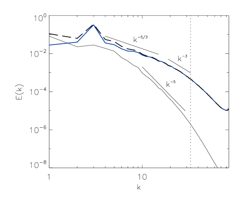
Figure 11: (Color online) Kinetic [thick (blue) line] and magnetic energy spectra (thin line) at $t=150$ in the simulation in set 9 with $R_{M}\approx 41$ ($P_{M}=0.0125$) in the saturated regime. The thick dashed line shows the total energy spectrum and the thin vertical dotted line the wavenumber at which the $\alpha$ filtering sets in. Note the compatibility of the spectra with a Kolmogorov law in the large scales for the kinetic spectrum, followed by a steeper power law.

In Refs. Mininni et al. (2005c); Mininni and Montgomery (2005) it was shown using different forcing functions that even at low $P_{M}$ the magnetic energy spectrum in the kinematic regime of the dynamo peaks at small scales. In these simulations, the critical magnetic Reynolds number $R_{M}^{c}$ was of the order of a few hundreds, and as a result small scales were excited. For ABC forcing, $R_{M}^{c}$ is of the order of a few tens and close to the threshold small scales are damped fast. Only large-scale dynamo action is observed and thus, even at early times, the magnetic energy spectrum peaks at large scales. However, if $R_{M}$ is increased above $R_{M}\approx 400$, a magnetic energy spectrum that peaks at scales smaller than the forcing scale (as in Refs. Mininni et al. (2005c); Mininni and Montgomery (2005)) is recovered. We focus here on large-scale dynamo action, and as a result will discuss the spectral evolution in simulations with $R_{M}$ of a few tens.

Figure 9 shows the evolution of the magnetic energy spectrum at different times for a run in set 6 with $R_{M}\approx 41$. As in previous studies, in the kinematic regime all the Fourier shells grow with the same rate. Then, magnetic saturation is reached and the mode at $k=1$ keeps growing until it eventually saturates itself. Figure 10 shows the kinetic and magnetic energy spectra at late times ($t=210$) after nonlinear saturation in the simulation in set 6 with $R_{M}\approx 41$ ($P_{M}=0.05$). At $k=1$ the system is dominated by magnetic energy, but at smaller scales the magnetic energy spectrum drops fast. The kinetic energy spectrum peaks at the forcing band ($k=3$) and then drops with a slope compatible with $k^{-3}$. This drop is due to the action of the Lorentz force that removes mechanical energy from the $k=3$ shell to sustain the magnetic field at $k=1$ Alexakis et al. (2005); Mininni et al. (2005d).

Figure 12: Spectrum of relative magnetic helicity $k^{-1}H_{M}(k)/E_{M}(k)$ at different times in the simulation in set 6 with $R_{M}\approx 41$ ($P_{M}=0.05$). The labels are as in Fig. 9. Note the evolution towards a force-free field at $k=1$, the small excess of positive helicity at scales slightly smaller than the forcing scale, and the absence of relative magnetic helicity in the small scales at all times.

A slope close to a $k^{-3}$ power law in the kinetic energy spectrum in the saturated regime at small scales is observed in several of the simulations with $P_{M}<1$. Simulations with small $P_{M}$ and larger values of $R_{V}$ were done using both the LAMHD equations and high-resolution DNS on grids of $512^{3}$ and $1024^{3}$ points (see Table 1). In these simulations, a power law close to $k^{-5/3}$ is observed before the kinetic energy spectrum drops to a steeper slope. As an example, Fig. 11 shows the kinetic and magnetic energy spectra in a simulation from set 9 using the LAMHD model, with $R_{M}\approx 41$ ($P_{M}=0.0125$). Slopes corresponding to $k^{-5/3}$, $k^{-3}$, and $k^{-5}$ are indicated as a reference in Fig. 11. A $k^{-5}$ power law in the magnetic energy spectrum (following a $k^{-3}$ range) was observed in experiments of dynamo action with constrained helical flows at low $R_{M}$ Müller et al. (2004); in addition, a $k^{-3}$ power law for the kinetic energy spectrum is consistent with the observed magnetic energy spectrum Léorat et al. (1981). Note that these power laws are only discussed here in order to be able to compare with the experimental data, but higher Reynolds numbers and thus more resolution will be needed in order to ascertain the spectral dependency of the flow and the magnetic field in the different inertial ranges of low $P_{M}$ simulations.

Figure 13: Spectrum of $H_{V}(k)-k^{2}H_{M}(k)$, proportional to (minus) the non-linear $\alpha$-effect, in the simulation in set 6 with $R_{M}\approx 41$ ($P_{M}=0.05$). The labels are as in Figs. 9 and 12: the solid line is for $t=11$, the dashed line for $t=29$, and the long dashed line for $t=120$. Note the drop of the spectrum at late times at scales smaller than $k_{F}$.

Figure 12 shows the spectrum of relative magnetic helicity $k^{-1}H_{M}(k)/E_{M}(k)$ at different times for the same run as in Figs. 9 and 10 (run with $R_{M}\approx 41$ in set 6). At all times, scales larger than the forcing scale have negative magnetic helicity, while scales of the order of, or smaller than the forcing scale have positive magnetic helicity. This is consistent with an inverse cascade of negative magnetic helicity at wavenumbers smaller than $k_{F}$, and with a direct transfer of positive magnetic helicity at wavenumbers larger than $k_{F}$, as analyzed in Alexakis et al. (2006) using transfer functions. The relative helicity in the $k=1$ shell grows with time until reaching saturation. Note that at late times, $H_{M}(k=1)/E_{M}(k=1)\approx-1$, indicating that the large scale magnetic field is nearly force-free.

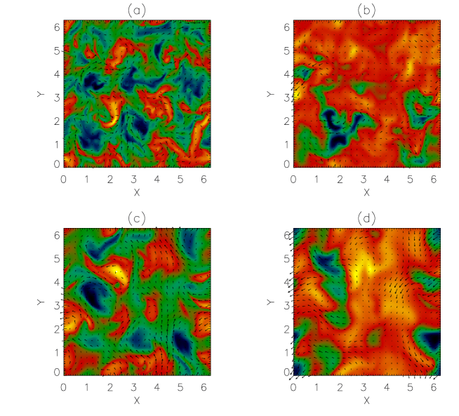
Figure 14: (Color online) Plots of the velocity and magnetic fields in a cut at $z=0$ for the simulation in set 6 with $R_{M}\approx 41$ and $R_{V}\approx 820$ ($P_{M}=0.05$): (a) $v_{z}$ component in color and $v_{x}$, $v_{y}$ indicated by arrows at early time, (b) same as in (a) for the magnetic field at early time, (c) same as in (a) at late time, and (d) same as in (b) at late time.

Figure 13 also shows the spectrum of $H_{V}(k)-k^{2}H_{M}(k)$, proportional to (minus) the non-linear $\alpha$-effect Pouquet et al. (1976). Three times are shown for the same run than in Figs. 9, 10, and 12 (set 6, $R_{M}\approx 41$). At early times ($t=11$ and $t=29$) the spectrum of $H_{V}(k)-k^{2}H_{M}(k)$ is close to the spectrum of the kinetic helicity. However, as the large scale magnetic field grows ($t=120$ is shown in the figure) the current helicity $k^{2}H_{M}(k)$ quenches kinetic helicity fluctuations and the total spectrum drops at scales smaller than $k_{F}$.

Figure 15: Saturation value of the magnetic energy in the $k=1$ shell, normalized by the total kinetic energy. The triangles correspond to simulations at constant $R_{V}$, while the squares correspond to simulations at constant $R_{M}$ (squares connected with solid lines are from DNS, while squares connected with dotted lines are from LAMHD simulations).

As a result, at late times the magnetic energy is mostly in the modes with wavenumber $k=1$, which corresponds to the largest available scale in the system. In addition, the large scale magnetic field is force-free (maximum relative helicity with $H_{M}(k)=E_{M}(k)$ at $k=1$. Figure 14 shows slices of the velocity and magnetic fields at early and late times. The growth of a large scale magnetic field and the quenching of turbulent velocity fluctuations in the saturated regime can be easily identified.

The situation resembles other inverse cascade situations that have been studied numerically, in which the fundamental $k=1$ mode dominates the dynamics at long times and its growth is only limited by its own dissipation rate Hossain et al. (1983); Brandenburg (2001); Mininni et al. (2003); Brandenburg and Subramanian (2005). In helical dynamo simulations at $P_{M}=1$ this behavior has also been observed, although it was speculated that for $P_{M}<1$ the inverse cascade of magnetic helicity and the generation of large scale fields should be quenched Brandenburg (2001). In fact, the generation of magnetic energy at scales larger than the forcing scale is not quenched as $P_{M}$ is decreased. This is illustrated in Fig. 15, which shows the ratio of the magnetic energy in the $k=1$ shell to the total kinetic energy in the saturated state as a function of $P_{M}$. Curves both at constant $R_{V}$ and constant $R_{M}$ are given. For constant $R_{M}$ and small $P_{M}$ the magnetic energy in the large scales seems to be independent of $P_{M}$ and $R_{V}$. The overall shape of the curves is similar to the curves in Fig. 7, indicating that at late times the evolution of the total magnetic energy is dominated by the magnetic field in the large scales.

IV Conclusion

We have shown in this paper that the phenomenon of inverse cascade of magnetic helicity, and the ensuing growth of large-scale magnetic energy together with a force-free magnetic field at large times, is present at low magnetic Prandtl number, down to $P_{M}=0.005$ in kinematic regime studies and down to $P_{M}=0.01$ in simulations up to the nonlinear saturation. The quenching of the velocity in the small scales, already observed in laboratory experiments, is also present. The augmentation of the critical magnetic Reynolds number as $R_{V}$ increases is less than in the non-helical case Schekochihin et al. (2004); Ponty et al. (2005); Schekochihin et al. (2005), and even smaller than what was found for helical flows when the large-scale dynamo is not permitted, as e.g. for the Roberts flow at $k\approx 1$ Mininni and Montgomery (2005). The reason for this difference is that in the present study we allowed for enough scale separation between the forcing scale and the largest scale for helical large-scale dynamo action to develop. The results are in agreement with studies using mean-field theory and shell models to study both large- and small-scale dynamo action Frick et al. (2006). Large-scale helical dynamo action in the $P_{M}<1$ regime requires much smaller magnetic Reynolds numbers to work than small-scale dynamos.

The challenge remains, numerically, to be able to reach values of the magnetic Prandtl number comparable to those found in geophysics and astrophysics and in the laboratory, i.e. $P_{M}\approx 10^{-5}$. However, it is unlikely that the dynamo instability found here down to $P_{M}=0.005$ would disappear as $P_{M}$ is lowered further. An open question, of importance from the experimental point of view when dealing with turbulent liquid metals, is whether the critical magnetic Reynolds number $R_{M}^{c}$ will stabilize, for a given flow, at a value intermediate between what it is at $P_{M}=1$ and the peak of the curve (see Fig. 1), or whether for large-scale helical dynamo action and extremely low values of $P_{M}$, it will go back down to the value it has at $P_{M}=1$. The data up to this day suggests the former, but on the other hand the study made in the context of two-point closures of turbulence Léorat et al. (1981) suggests the latter. This also means that reliable models of turbulent flows in MHD must be developed in order that we can explore in a more systematic way the parameter space characteristic of the flows of interest, as for the geo-dynamo or the solar dynamo.