Abstract

Within a simple model context, the sensitivity and stability of the thermohaline circulation to finite amplitude perturbations is studied. A new approach is used to tackle this nonlinear problem. The method is based on the computation of the so-called Conditional Nonlinear Optimal Perturbation (CNOP) which is a nonlinear generalization of the linear singular vector approach (LSV). It is shown that linearly stable thermohaline circulation states can become nonlinearly unstable and the properties of the perturbations with optimal nonlinear growth are determined. An asymmetric nonlinear response to perturbations exists with respect to the sign of finite amplitude freshwater perturbations, on both thermally dominated and salinity dominated thermohaline flows. This asymmetry is due to the nonlinear interaction of the perturbations through advective processes.

Key words: thermohaline circulation, conditional optimal nonlinear perturbation, nonlinear stability, sensitivity

1 Introduction

A recurrent theme in fundamental research on climate variability is the sensitivity of the ocean’s thermohaline circulation. When state-of-the-art climate models are used to calculate projections of future climate states as a response to different emission scenarios of greenhouse gases, a substantial spread in the model results is found. One of the reasons of this spread is the diverse behavior of the thermohaline circulation McAvaney (2001).

The sensitivity of the thermohaline circulation is caused by several feedbacks induced by the physical processes that determine the evolution of the thermohaline flow. One of these feedbacks is the salt-advection feedback which is caused by the fact that salt is transported by the thermohaline flow, but in turn influences the density difference which drives this flow. The salt-advection feedback can be conceptually understood in a two-box model Stommel (1961) where it is shown to cause multiple equilibria and hysteresis behavior.

In many models of the global ocean circulation, it appears that several equilibrium states may exist under similar forcing conditions. When the present equilibrium state, with about 16 Sv Atlantic overturning, is subjected to a quasi-steady freshwater input in the North Atlantic, eventually the circulation may collapse. In this collapsed state, there is deepwater formation in the Southern Ocean instead of in the North Atlantic and the formation of North Atlantic Deep Water (NADW) has ceased Stocker et al. (1992); Rahmstorf (1995); Manabe and Stouffer (1999). As this multiple equilibrium regime seems to be present in many ocean models, it is important to determine whether transitions between the different states can occur due to finite amplitude perturbations.

In a variant of the Stommel-model for which the temperature relaxation is fast, Cessi (1994) studied the transition behavior between the different equilibria. In this case, there are only three equilibrium states, of which one unstable. In the deterministic case, she finds that a finite amplitude perturbation of the freshwater flux can shift the system into an alternate state and that the minimum amplitude depends on the duration of the disturbance. Regardless of the duration, however, the amplitude of the disturbance has to exceed a certain value for a transition to occur. Under stochastic white-noise forcing, there are occasional transitions from one equilibrium to another as well as fluctuations around each state.

In Timmermann and Lohmann (2000), the effect of multiplicative noise (through fast fluctuations in the meridional thermal temperature gradient) on the variability in a box model similar to that in Cessi (1994) has been studied. It was found that the stability properties of the thermohaline circulation depend on the noise level. Red noise can introduce new equilibria that do not have a deterministic counterpart.

Another line of studies uses box models that show intrinsic variability because of the existence of an oscillatory mode in the eigenspectrum of the linear operator. Griffies and Tziperman (1995) show that noise is able to excite an otherwise damped eigenmode of the thermohaline circulation. Tziperman and Ioannou (2002) study the non-normal growth of perturbations on the thermally driven state and identify two physical mechanisms associated with the transient amplification of these perturbations.

Stochastic noise can have a significant effect on the mean states of the thermohaline circulation and their stability Hasselmann (1976); Palmer (1995); Vélez-Belchí et al. (2001); Tziperman and Ioannou (2002). Some of these mechanisms are intrinsically linear, such as the effects of non-normal growth considered in Tziperman and Ioannou (2002). Others are essentially nonlinear mechanisms, such as those causing the noise-induced transitions reported in Timmermann and Lohmann (2000).

To study linear amplification mechanisms, the linear singular vector (LSV) method is often used, with main applications to predictability studies Xue and Zebiak (1997a, b); Thompson (1998). Knutti and Stocker (2002), for example, found that the sensitivity of the ocean circulation to perturbations severely limits the predictability of the future thermohaline circulation when approaching the bifurcation point. The LSV approach, however, cannot provide critical boundaries on finite amplitude stability of the thermohaline ocean circulation.

In a system which potentially has multiple equilibria and internal oscillatory modes, its response to a finite amplitude perturbation on a particular steady state is a difficult nonlinear problem. In this paper, we determine the nonlinear stability boundaries of linearly stable thermohaline flow states within a simple box model of the thermohaline circulation. To compute these boundaries, we use the concept of the Conditional Nonlinear Optimal Perturbation (CNOP) and study optimal nonlinear growth over a certain given time $\tau$. We extend results on linear optimal growth properties of perturbations on both thermally and salinity dominated thermohaline flows to the nonlinear case. We find that there is an asymmetric nonlinear response of these flows with respect to the sign of the finite amplitude freshwater perturbation and describe a physical mechanism that explains this asymmetry.

2 Model and methodology

a. Model

To illustrate the approach, the theory is applied to a 2-box model of the thermohaline circulation Stommel (1961). This model consists of an equatorial box and a polar box which contain well mixed water of different temperatures and salinities due to an equatorial-to-pole gradient in atmospheric surface forcing. Flow between the boxes is assumed proportional to the density difference between the boxes and, with a linear equation of state, related to the temperature and salinity differences in the boxes.

When the balances of heat and salt are nondimensionalized, the governing dimensionless equations (we use the notation in chapter 3 of Dijkstra (2000)) can be written as

$$\frac{dT}{dt}&=\eta_{1}-T(1+\mid T-S\mid)\\ \frac{dS}{dt}=\eta_{2}-S(\eta_{3}+\mid T-S\mid)$$ (1)

where $T=T_{e}-T_{p},~{}S=S_{e}-S_{p}$ are the dimensionless temperature and salinity difference between the equatorial and polar box and $\Psi=T-S$ is the dimensionless flow rate. Three parameters appear in the equations (1): the parameter $\eta_{1}$ measures the strength of the thermal forcing, $\eta_{2}$ that of the freshwater forcing and $\eta_{3}$ is the ratio of the relaxation times of temperature and salinity to the surface forcing. Steady states of the equations (1) are indicated with a temperature of $\bar{T}$, a salinity of $\bar{S}$ and a flow rate $\bar{\Psi}=\bar{T}-\bar{S}$. A steady state is called thermally-dominated when $\bar{\Psi}>0$, i.e. a negative equatorial-to-pole temperature gradient exists dominating the density. A steady state is called salinity-dominated when $\bar{\Psi}<0$, i.e. a negative equatorial-to-pole salinity gradient exists dominating the density.

It is well known that the equations (1) have multiple steady states for certain parameter values. Here, we fix $\eta_{1}=3.0$, $\eta_{3}=0.2$ and use $\eta_{2}$ as control parameter. The bifurcation diagram for these parameter values is shown in Fig. 1 as a plot of $\bar{\Psi}$ versus $\eta_{2}$. Solid curves indicate linearly stable steady states, whereas the states on the dashed curve are unstable. There are thermally-driven (hereafter TH) stable steady states ($\bar{\Psi}>0$) and salinity-driven (hereafter SA, ie., the circulation is salinity-dominated) stable steady states ($\bar{\Psi}<0$). The saddle-node bifurcation points occur at $\eta_{2}=0.600$ and $\eta_{2}=1.052$, and bound the interval in $\eta_{2}$ where multiple equilibria occur. Suppose that this bifurcation diagram represents both the present overturning state (on the stable branch with $\bar{\Psi}>0$) and the collapsed state (on the stable branch with $\bar{\Psi}<0$). To study the nonlinear transition behavior of the thermohaline flows from the TH state to the SA state and vice versa, we consider the evolution of finite amplitude perturbations on the stable states.

The nonlinear equation governing the evolution of perturbations can be derived from equation (1). If the steady state ($\bar{T},\bar{S}$) is given and $T^{\prime}=T-\bar{T}$, $S^{\prime}=S-\bar{S}$ are the perturbations of temperature and salinity, then it is found that

$$\frac{dT^{\prime}}{dt}&=-(2|\bar{\Psi}|+1)T^{\prime}+sign(\bar{\Psi})[\bar{T}\,S^{\prime}-\bar{S}T^{\prime}-T^{\prime}(T^{\prime}-S^{\prime})]\\ \frac{dS^{\prime}}{dt}=-(2|\bar{\Psi}|+\eta_{3})S^{\prime}+sign(\bar{\Psi})[\bar{T}\,S^{\prime}-\bar{S}T^{\prime}-S^{\prime}(T^{\prime}-S^{\prime})]$$ (2)

where $sign(\bar{\Psi})$ is sign of steady flow rate $\bar{\Psi}$. If the perturbations are sufficiently small, such that the nonlinear part of the equations (2) can be neglected, we find the tangent linear equation governing the evolution of small perturbations as

$$\frac{dT^{\prime}}{dt}&=-(2|\bar{\Psi}|+1)T^{\prime}+sign(\bar{\Psi})(\bar{T}\,S^{\prime}-\bar{S}T^{\prime})\\ \frac{dS^{\prime}}{dt}=-(2|\bar{\Psi}|+\eta_{3})S^{\prime}+sign(\bar{\Psi})(\bar{T}\,S^{\prime}-\bar{S}T^{\prime})$$ (3)

b. Conditional Nonlinear Optimal Perturbation

To study nonlinear mechanisms of amplification, Berloff and Meacham (1996) modified the LSV technique and Mu (2000) proposed the concept of nonlinear singular vectors (NSVs) and nonlinear singular values (NSVAs). These concepts were successfully applied by Mu and Wang (2001) and Durbiano (2001) to study finite amplitude stability of flows in two-dimensional quasi-geostrophic and shallow-water models, respectively. In Mu and Duan (2003), the concept of the conditional nonlinear optimal perturbation (CNOP) was introduced and applied to study the “spring predictability barrier” in the El Nino-Southern Oscillation (ENSO), using a simple equatorial ocean-atmosphere model. The “spring predictability barrier” refers to the dramatical decline of the prediction skills for most of the ENSO models during the Northern Hemisphere (NH) springtime. The CNOP can also be employed to estimate the prediction errors of an El Niño or a La Niña event Mu et al. (2003).

As readers may not be familiar with this concept, we give a brief introduction to CNOP. Considering the nonlinear evolution of initial perturbations governed by (2). In general, assume that the equations governing the evolution of perturbations can be written as:

$$\begin{array}[]{ll}\left\{\begin{array}[]{l}\displaystyle\frac{\partial{\textbf{{x}}}}{\partial t}+F(\textbf{{x}};\bar{\textbf{{x}}})=0,\\[5.69046pt] {\textbf{{x}}}|_{t=0}={\textbf{{x}}}_{0},\\ \end{array}\right.&\ \ \ {\rm in}\ \ \ \Omega\times[0,t_{e}]\end{array}$$ (4)

where $t$ is time, ${\textbf{{x}}}(t)=(x_{1}(t),x_{2}(t),...,x_{n}(t))$ is the perturbation state vector and $F$ is a nonlinear differentiable operator. Furthermore, ${\textbf{{x}}_{0}}$ is the initial perturbation, $\bar{\textbf{{x}}}$ is the basic state, $({\textbf{{x}}},t)\in\Omega\times[0,t_{e}]$ with $\Omega$ a domain in $R^{n}$, and $t_{e}<+\infty$.

Suppose the initial value problem (4) is well-posed and the nonlinear propagator $M$ is defined as the evolution operator of (4) which determines a trajectory from the initial time $t=0$ to time $t_{e}$. Hence, for fixed $t_{e}>0$, the solution ${\textbf{{x}}}(t_{e})=M({\textbf{{x}}_{0};\bar{\textbf{{x}}}})(t_{e})$ is well-defined, i.e.

$$\textbf{{x}}(t_{e})=M(\textbf{{x}}_{0};\bar{\textbf{{x}}})(t_{e})$$ (5)

So $\textbf{{x}}(t_{e})$ describes the evolution of the initial perturbation ${\textbf{{x}}}_{0}$.

For a chosen norm $\|\cdot\|$ measuring x, the perturbation ${\textbf{{x}}}^{\*}_{0\delta}$ is called the Conditional Nonlinear Optimal Perturbation (CNOP) with constraint condition $\|{\textbf{{x}}}_{0}\|\leq\delta$ , if and only if

$$J({\textbf{{x}}}^{\*}_{0\delta})=\max_{\|{\textbf{{x}}}_{0}\|\leq\delta}J({\textbf{{x}}}_{0})$$ (6)

where

$$J({\textbf{{x}}}_{0})=\|M({\textbf{{x}}}_{0};\bar{\textbf{{x}}})(t_{e})\|$$ (7)

The CNOP is the initial perturbation whose nonlinear evolution attains the maximal value of the functional $J$ at time $t_{e}$ with the constraint conditions; in this sense we call it “optimal”. The CNOP can be regarded as the most (nonlinearly) unstable initial perturbation superposed on the basic state. With the same constraint conditions, the larger the nonlinear evolution of the CNOP is, the more unstable the basic state is. In general, it is difficult to obtain an analytical expression of the CNOP. Instead we look for the numerical solution, by solving a constraint nonlinear optimization problem.

To calculate the CNOP the norm

$$\|{\textbf{{x}}}_{0}\|=\sqrt{(T^{\prime}_{0})^{2}+(S^{\prime}_{0})^{2}}$$ (8)

is used. Using a fourth-order Runge-Kutta scheme with a time step $dt=0.001$, perturbation solutions $(T^{\prime},S^{\prime})$ are obtained numerically by integrating the model (2) up to a time $t_{e}$ and the magnitude of the perturbation is calculated. Next, the Sequential Quadratic Programming (SQP) method is applied to obtain the CNOP numerically; the SQP method is briefly described in the Appendix.

To compare the CNOPs with the LSVs, the latter are also computed using the theory of linear singular vector analysis Chen et al. (1997). We also use the norm (8) in this analysis and first solve (3) to obtain the linear evolution of initial perturbations. Subsequently, the singular vector decomposition (SVD) is used to determine the linear singular vectors (LSVs) of the model.

3 Stability and sensitivity analysis

In this section, we compute the CNOPs to study the sensitivity of the thermohaline circulation to finite amplitude freshwater perturbations in the two-box model. Two problems are studied: (i) the nonlinear development of the finite amplitude perturbations for fixed parameters in the model and (ii) the nonlinear stability of the steady states as parameters are changed. Both thermally-dominated steady states ($\bar{\Psi}>0$) and salinity-dominated ones ($\bar{\Psi}<0$) are investigated. The initial perturbation $\textbf{{x}}_{0}$ is written as $\textbf{{x}}_{0}=(T^{\prime}_{0},S^{\prime}_{0})=(\delta\cos\theta,\delta\sin\theta)$ , where $\delta$ is magnitude of initial perturbation and $\theta$ the angle of the initial vector with the x-axis.

3.1 Finite amplitude evolution of the TH state

For the thermally-driven stable steady state, we consider the state $\bar{T}=1.875,\bar{S}=1.275,\bar{\Psi}=0.6$ (shown as point ”A” in Fig. 1) with the fixed parameters $\eta_{1}=3.0$, $\eta_{2}=1.02$, $\eta_{3}=0.2$. We choose $t_{e}=2.5$ and use $\delta=0.3$ as a maximum norm (in the norm (8)) of the perturbations. The time $t_{e}$ is about half the time the solution takes to equilibrate to steady state from a particular initial perturbation. The amplitude $\delta=0.3$ is about $10\%$ of the typical amplitude of the steady state of temperature and salinity $(\bar{T},\bar{S})$. For $\theta$ in the range $\pi/4<\theta<5\pi/4$, the initial perturbation flow has $\Psi^{\prime}(0)<0$. As this is typically caused by a freshwater flux perturbation in the polar box, we refer to the perturbation as being of freshwater type. For other angles $\theta\in[0,2\pi]$ , the initial perturbation flow has $\Psi^{\prime}(0)>0$, which is typically caused by a salt flux perturbation in the polar box and we refer to it as being of salinity type.

Using equation (2) and (3), both CNOPs and LSVs are computed versus the constraint condition $\delta$, respectively. The numerical results, plotted in Fig. 2, indicate that the CNOPs are located at the circle $\|\textbf{{x}}_{0}\|=\delta$, which is the boundary of ball $\|\textbf{{x}}_{0}\|\leq\delta$. The directions of the LSVs, which are independent of $\delta$, have constant values of $\theta_{1}=1.948$ (dashed line) and $\theta_{2}=5.089$ (not shown). The value of $\theta$ for the CNOPs (solid curve) increases monotonically over the $\delta$ interval 0.01 to 0.3. The difference between CNOPs and LSVs is relatively small when $\delta$ is small.

Integrating the model (2) with CNOPs and LSVs as initial conditions, respectively. we obtain their evolutions at time $t_{e}$, which are denoted as ”CNOP-N” and ”LSV-N”; these are shown in Fig. 3. For comparison, the linear evolution of the LSVs are also obtained by integrating the model (3) with the LSV as an initial condition; this is denoted as ”LSV-L” in Fig. 3. It is clear that the evolution of the CNOPs is nonlinear in $\delta$, while ”LSV-L” only increases linearly. The line of ”LSV-N” is between ”CNOP-N” and ”LSV-L”, but the difference between ”LSV-N” and ”CNOP-N” is hardly distinguishable over the whole $\delta$ interval. Though this difference is not significant in this TH state, it is significant in the following investigation for SA state. In fact, it is very hard to know this without previous calculation.

Note that since our numerical results demonstrate that the CNOPs are all located on the boundary $\|{\textbf{{x}}}_{0}\|=\delta$, we are able to show the sensitivity of THC to finite amplitude perturbations of specific fixed amplitude $\delta=0.2$. In Fig. 4 the value of $J$ at $t_{e}=2.5$ is shown for the linear and the nonlinear evolutions of the initial perturbations obtained by (2) and (3). For the linear case (dashed line in Fig. 4), there are two optimal linear initial perturbations $\theta_{1}=1.948$ and $\theta_{2}=5.089$ with the same value of $J$, $J(\delta,\theta_{1})=J(\delta,\theta_{2})=0.16484$, which are the LSVs. Note that $\theta_{2}-\theta_{1}=\pi$, which means that in the linear case perturbations with $\Psi^{\prime}>0$ and $\Psi^{\prime}<0$ behave similarly (and hence symmetrically with respect to the sign of $\Psi^{\prime}$). For the nonlinear model (solid curve in Fig. 4), there is one global optimal nonlinear initial perturbation with $\theta_{3}=1.979$, which is the CNOP, and one local optimal nonlinear initial perturbations at $\theta_{4}=5.058$, with values of $J(\delta,\theta_{3})=0.22413$ and $J(\delta,\theta_{4})=0.13052$, respectively. The results in Fig. 4 for $\delta=0.2$ coincide with the results in Fig. 2.

There is another difference between the linear and nonlinear evolution of the perturbations. When the initial perturbations are freshwater ($\Psi^{\prime}<0$), the nonlinear evolution leads to a larger amplitude than the linear evolution. When the initial perturbations are saline ($\Psi^{\prime}>0$), the nonlinear evolution leads to a smaller amplitude than the linear evolution. For example, the initial perturbations with $\theta_{1}$ and $\theta_{3}$ are such that $\Psi^{\prime}<0$, while the initial perturbations with $\theta_{2}$ and $\theta_{4}$ have $\Psi^{\prime}>0$.

The values of $J/\delta$ obtained by integrating (2) with the CNOPs as initial condition are shown for different $\delta$ in Fig. 5a. The corresponding evolution of $\Psi$ is plotted in Fig. 5b. To relate the result in Fig. 5a to previous ones, consider the value of $J/\delta$ at $t=2.5$ on the curve of $\delta=0.2$. In Fig. 4, the maximum of $J$ is 0.224 and hence $J/\delta=0.224/0.2=1.12$. It follows from the Figs. 5 that for the CNOP with $\delta=0.01$, the flow rate $\Psi$ recovers to the steady state $\bar{\Psi}=0.6$ rapidly. For the CNOP with a larger initial amplitude ($\delta=0.1,0.2$), it takes much longer for the thermohaline circulation to recover to steady state. This is different from a linear analysis where the evolution is the same for all optimal initial perturbations Tziperman and Ioannou (2002).

In summary, the results for the TH state show that fresh perturbations, with $\Psi^{\prime}<0$, are more amplified though nonlinear mechanisms than saline perturbations, with $\Psi^{\prime}>0$. This is consistent with the notion that perturbations which move the system towards a bifurcation point will be more amplified through non-linear mechanisms than perturbations that move the system away from a bifurcation point.

3.2 Finite amplitude stability of the SA state

We consider the salinity-dominated SA state ($\bar{T}=2.674,\bar{S}=2.796,\bar{\Psi}=-0.122$) for a slightly smaller value of $\eta_{2}$ than for the thermally-dominated TH state in the previous section ($\eta_{1}=3.0$, $\eta_{2}=0.9$, $\eta_{3}=0.2$). It is indicated as point ”B” in Fig. 1. Again for the time $t_{e}=2.5$, using the corresponding equations (2) and (3), both CNOPs and LSVs are computed versus the constraint condition $\delta$, respectively and the results are plotted in Fig. 6.

Similar to the results in Fig. 2, the directions of the LSVs, which are independent of $\delta$, have constant values of $\theta_{1}=2.796$ and $\theta_{2}=5.938$ (dashed line). The line for $\theta_{1}$ is similar to $\theta_{2}$, and is not drawn in Fig. 6. The direction of CNOPs (solid curve) increase monotonously with $\delta$ varying from 0.01 to 0.125. Then, $\theta$ drops down to $2.857$ at $\delta=0.125$ and increase slightly with $\delta$ in the interval $0.125<\delta<0.17$. After that, $\theta$ jumps up to $5.195$ at $\delta=0.17$ and increases slightly with $\delta$ in $0.17<\delta<0.22$.

Using equations (2) and (3), the evolutions of both the CNOPs and LSVs of the SA state are shown in Fig. 7. All the three kinds of evolutions are approximately the same when the initial perturbations are relatively small. But for larger $\delta$ the difference between ”LSV-N” and ”CNOP-N” is remarkably larger than that of the TH state (Fig. 3). The values of $J$ of ”CNOP-N” are always larger than those of both ”LSV-L” and ”LSV-N” for $\delta>0.17$.

The values of $J$ at a time $t_{e}=2.5$ for all $\theta$ show (Fig. 8a) two optimal linear initial perturbations $\theta_{1}=2.796$ and $\theta_{2}=5.938$ with $J(\delta,\theta_{1})=J(\delta,\theta_{2})=0.0526$. Again, because $\theta_{2}-\theta_{1}=\pi$ there is the symmetry in response with respect to the sign of $\Psi^{\prime}$. For nonlinear evolutions, there is one globally optimal initial perturbation at $\theta_{3}=5.246$ (the CNOP) and two locally optimal initial perturbations at $\theta_{4}=0.251$ and $\theta_{5}=2.890$, with J-values of $J(\delta,\theta_{3})=0.0963$, $J(\delta,\theta_{4})=0.0432$ and $J(\delta,\theta_{5})=0.0503$, respectively. The initial perturbations with $\theta_{1}$ and $\theta_{5}$ are of freshwater type ($\Psi^{\prime}<0$), while the initial perturbations of $\theta_{2}$, $\theta_{3}$ and $\theta_{4}$ are of salinity type ($\Psi^{\prime}>0$).

To understand the difference between the maxima located at $\theta_{3}$, $\theta_{4}$ and $\theta_{5}$, a contour graph of $J(\theta,\delta)$ is drawn in Fig. 8b. It is clear from Fig. 8b that there are three groups of local maxima which are indicated by the dashed lines. When $\delta<0.125$ there are only two local maxima and the CNOP is located in the regime $5\pi/4<\theta<2\pi$. When $0.125<\delta<0.17$, the CNOP jumps from the interval $5\pi/4<\theta<2\pi$ to the interval $3\pi/4<\theta<5\pi/4$. This coincides with the jumping behavior of $\theta$ in Fig. 6. When $\delta>0.17$, there are three local maxima and the CNOP jumps from the interval $3\pi/4<\theta<5\pi/4$ to a new interval $5<\theta<6$. Both jumps are also shown in Fig. 6 and $J$ has a remarkable increase after the second jump (Fig. 7).

Also for the SA state, the value of $J/\delta$ along trajectories obtained by integrating equations (2) using the CNOPs as initial conditions are shown for different $\delta$ in Fig. 9a. The corresponding evolution of $\Psi$ is plotted in Fig. 9b. For $t=2.5$ and $\delta=0.2$, the value of $J/\delta=0.0963/0.2=0.48$, where 0.0963 is the maximum in Fig. 8a. The flow rate $\Psi$ recovers to the steady state (whose value is $-0.122$) shortly after being disturbed with a small amplitude CNOP ($\delta=0.01$). It takes much longer for the thermohaline circulation to recover to the steady state after being disturbed with a larger amplitude ($\delta=0.1,0.2$), respectively. The larger the CNOP is, the larger the transient effect. In contrast to the TH state, there is now an oscillatory attraction to the SA state, already described in Stommel (1961).

In both the salinity-dominated SA state and the thermally-dominated TH state, the CNOP always moves the system towards the bifurcation point. The SA state (TH state) has an asymmetry in the nonlinear amplification of disturbances, with a larger amplification for those with $\Psi^{\prime}>0$ ($\Psi^{\prime}<0$).

3.3 Sensitivity along the bifurcation diagram

Even if a TH or SA state is linearly stable, it can become nonlinearly unstable due to finite amplitude perturbations. The methodology of CNOP provides a means to assess the nonlinear stability thresholds of the thermohaline flows; here this is shown for the two-box model (2). Thereto, we compute the CNOPs under different $\delta$ constraints for linearly stable TH and SA states along the bifurcation diagram in Fig. 1.

Along the TH branch, we vary $\eta_{2}$ from 1.043 to 1.046 with step 0.001 and thereby approach the saddle-node bifurcation (Fig. 1). For each value of $\eta_{2}$, the CNOPs are obtained under the constraint that the magnitude of initial perturbations is less 0.2 ($\delta=0.2$) and again the time $t_{e}=2.5$. The trajectories of the CNOPs are calculated by integrating the model (2) (Fig. 10a). Next, the corresponding flow rates $\Psi$ are drawn in Fig. 10b. Both figures indicate that the CNOPs damp after a while for the steady states labelled $A_{1}$, $A_{2}$ and $A_{3}$. While these three states are consequently nonlinearly stable, the CNOP for steady state $A_{4}$ ($\eta_{2}=1.046$) increases in time, which implies that this steady state is nonlinearly unstable (although it is linearly stable) to perturbations with $\delta=0.2$.

From the above results, it follows that for each value of $\eta_{2}$, in the multiple equilibria regime of Fig. 1, a critical value of $\delta$, say $\delta_{c}$, must exists such that the TH state is nonlinearly unstable. $\delta_{c}$ is defined as the smallest magnitude of a finite amplitude perturbation which induces a transition from the TH state to the SA state. The larger the value of $\delta_{c}$, the more stable the steady state is. Using the CNOP method, the values of $\delta_{c}$ can be computed and the results for the TH states (from $\eta_{2}=0.95$ up to the saddle-node bifurcation at $\eta_{2}=1.052$ ) are shown in Fig. 11. The curve separates the plane into two parts. For the regime under the curve the steady state is nonlinearly stable and for the regime above the curve it is nonlinearly unstable. When the bifurcation point $Q$ in Fig. 1 is approached, $\delta_{c}$ decrease more and more quickly. The critical value $\delta_{c}$ reduces to zero sharply, as $\eta_{2}$ approaches the bifurcation point. This explains how the steady states lose their stability when the bifurcation point $Q$ is reached.

The same calculations are performed for steady states on the SA branch, when $\eta_{2}$ varies from 0.75 to the value 0.60 at the saddle-node bifurcation. The CNOPs are obtained under the constraint that the magnitude of initial perturbations is less than 0.1 ($\delta=0.1$) with time $t_{e}=2.5$. The trajectories of the CNOPs at each steady state (of which $J$ and $\Psi$ are plotted in Fig. 12) indicate that the CNOPs damp for the steady states labelled $B_{1}$, $B_{2}$ and $B_{3}$. Although there is oscillatory behavior, these states are nonlinearly stable. However, the evolution of CNOP for steady state $B_{4}$ ($\eta_{2}=0.70$) increases, which implies that the SA state is nonlinearly unstable to this finite amplitude perturbation (although it is linearly stable).

The critical boundaries $\delta_{c}$ for the SA states (Fig. 13) show that $\delta_{c}$ decreases monotonically with $\eta_{2}$ and becomes zero at saddle-node bifurcation ($\eta_{2}=0.6$). Similar to Fig. 11, the curve separates the plane into two parts. For the regime under the curve the steady state is nonlinearly stable and for the regime above the curve it is nonlinearly unstable. When $\eta_{2}$ decreases from $1.0$ to $0.6$, the SA steady states approach the bifurcation point $P$ in Fig. 1, and the critical value $\delta_{c}$ tends to zero. This explains how the steady states lose their stability at the bifurcation point $P$.

4 Summary and Discussion

Within a simple two-box model, we have addressed the sensitivity and nonlinear stability of (linearly stable) steady states of the thermohaline circulation. One of the remarkable results obtained by the CNOP approach is the asymmetry in the nonlinear amplification of perturbations with $\Psi^{\prime}<0$ (interpreted as a freshwater perturbation in the northern North Atlantic) and $\Psi^{\prime}>0$ (interpreted as a salt perturbation in the northern North Atlantic).

When we use LSV analysis, there are two singular vectors $x_{1}$ and $-x_{1}$ that correspond to one singular value $\sigma_{1}$ (see Fig. 4 and Fig. 8a). If $x_{1}$ is a freshwater type perturbation ( $\Psi^{\prime}<0$ ), $-x_{1}$ must be a salinity type perturbation ( $\Psi^{\prime}>0$ ). The conclusion from the linear analysis (using LSV) is that the thermohaline circulation is equally sensitive to either freshwater or salinity entering the northern North Atlantic. However, the nonlinear analysis (using CNOP) clearly reveals a difference in the response of the system to the two types of perturbations.

The asymmetry can be understood by considering the nonlinear evolution of perturbations in the two-box model. For the TH state, according to (2), the flow rate perturbation $\Psi^{\prime}=T^{\prime}-S^{\prime}$ satisfies

$$\frac{d\Psi^{\prime}}{dt}=(2\bar{S}-2\bar{T}-1)T^{\prime}+(2\bar{T}-2\bar{S}+\eta_{3})S^{\prime}-\Psi^{\prime 2}$$ (9)

Integrating the above equation, we find

$$\Psi^{\prime}(t)=\Psi^{\prime}(0)+\int_{0}^{t}L(T^{\prime},S^{\prime})d\tau-\int_{0}^{t}\Psi^{\prime 2}d\tau$$ (10)

where $L(T^{\prime},S^{\prime})$ is the linear part of (9). It is well known that the two linear terms in (9) determine the linear stability of the steady state Stommel (1961).

For an initial perturbation $\Psi^{\prime}(0)<0$ (freshwater type), the nonlinear term is always negative and the freshwater perturbation is amplified. This is a positive feedback and the stronger the freshwater perturbation, the stronger the nonlinear feedback destabilizing the TH steady state. A perturbation $\Psi^{\prime}(0)>0$ (salinity type) is damped by the negative definite nonlinear term. This is a negative feedback and the stronger the salinity perturbation, the stronger the nonlinear feedback stabilizing the TH state. Nonlinear mechanisms hence make the TH steady state more stable to salinity perturbations.

This explains the results in Fig. 4. For the freshwater type initial perturbations ($\Psi^{\prime}<0$), the nonlinear evolution of the initial perturbation of (2) is larger than the linear evolution of the initial perturbation of (3). For the salinity type initial perturbations ($\Psi^{\prime}>0$), the nonlinear evolution is smaller than the linear evolution. In general, the nonlinear term yields positive (negative) feedback for negative (positive) $\Psi^{\prime}$ in the case of thermally-dominated (TH) steady states.

On the other hand, when the basic steady flow is a SA state ($\bar{\Psi}<0$), then we have

$$\frac{d\Psi^{\prime}}{dt}=(2\bar{T}-2\bar{S}-1)T^{\prime}+(2\bar{S}-2\bar{T}+\eta_{3})S^{\prime}+\Psi^{\prime 2}$$ (11)

Similarly, we have,

$$\Psi^{\prime}(t)=\Psi^{\prime}(0)+\int_{0}^{t}L(T^{\prime},S^{\prime})d\tau+\int_{0}^{t}\Psi^{\prime 2}d\tau$$ (12)

Hence, due to nonlinear effects the SA steady state becomes more unstable (stable) to disturbances $\Psi^{\prime}>0$ ($\Psi^{\prime}<0$) which explains the results in Fig. 8a. In general, the nonlinear term yields positive (negative) feedback for positive (negative) $\Psi^{\prime}$ in the case of salinity-dominated (SA) steady states.

The physical mechanism behind the loss of stability of the TH state is often discussed in terms of the salt-advection feedback Marotzke (1995). A freshwater (salt) perturbation in the northern North Atlantic decreases (increases) the northward circulation and hence decreases (increases) the northward salt transport. The salt-advection feedback is independent of the sign of the perturbation of the flow rate $\Psi^{\prime}$. In contrast, the nonlinear instability mechanism of the thermohaline circulation depends on the sign of the perturbation of the flow rate $\Psi^{\prime}$ as discussed above.

The CNOP approach also allows us to determine the critical values of the finite amplitude perturbations (i.e. $\delta_{c}$) at which the nonlinearly induced transitions can occur. The techniques are currently being generalized to be able to apply them to models of the thermohaline circulation with more degrees of freedom. The aim is to tackle these problems eventually in global ocean circulation models. When applied to the latter models, the approach may provide quantitative bounds on perturbations of the present thermohaline flow such that nonlinear instability can occur.

Acknowledgments:  This work was supported by the National Natural Scientific Foundation of China (Nos. 40233029 and 40221503), and KZCX2-208 of the Chinese Academy of Sciences. It was initiated during a visit of HD to Beijing in the Summer of 2002 which was partially supported from a PIONIER grant from the Netherlands Organization of Scientific Research (N.W.O.). We also appreciate the valuable suggestions by anonymous reviewers.

Appendix: The SQP method

The constrained nonlinear optimization problem considered in this paper, after discretization and proper transformation of the objective function $F$, can be written in the form

$$\min_{x\in R^{n}}F(x),$$

subject to

$$c_{i}(x)\leq 0,\ \ \ \mathrm{for}\ i=1,2,3,\cdots,n,$$

where the $c_{i}$ are constraint functions. It is assumed that first derivatives of the problem are known explicitly, i.e., at any point $x$, it is possible to compute the gradient $\bigtriangledown F(x)$ of $F$ and the Jacobian $J(x)=\frac{\partial(c_{1},c_{2},\cdots,c_{n})}{\partial(x_{1},x_{2},\cdots,x_{n})}$ of the constraint functions $c_{i}$.

The SQP method is an iterative method which solves a quadratic programming (QP) subproblem at each iteration and it involves outer and inner iterations. The outer iterations generate a sequence of iterates $(x^{k},\lambda^{k})$ that converges to $(x^{*},\lambda^{*})$, where $x^{*}$ and $\lambda^{*}$ are respectively a constrained minimizer and the corresponding Lagrange multipliers. At each iterate, a QP subproblem is used to generate a search direction towards the next iterate $(x^{k+1},\lambda^{k+1})$. Solving such a subproblem is itself an iterative procedure, which is therefore regarded as a inner iterate of a SQP method. The following is an outline of the SQP algorithm used in this paper.

Step 1. Given a starting iterate $(x^{0},\lambda^{0})$ and an initial approximate Hessian $H^{0}$, set $k=0$.

Step 2. Minor iteration. Solve $d_{k}$ by the following QP subproblem.

$$\min_{d}([\nabla F(x^{k})]^{\top}d^{k}+\frac{1}{2}(d^{k\top}H^{k}d^{k})),$$

subject to

$$c(x^{k})+[\nabla c(x^{k})]^{\top}d^{k}\leq 0,$$

where $d^{k}$ is a direction of descent for the objective function.

Step 3. Check if $(x^{k},\lambda^{k})$ satisfies the convergence criterion, if not set $x^{k+1}=x^{k}+\alpha d^{k}$, where $\alpha\leq 1$. For $\lambda^{k+1}$, it is also determined by $d^{k}$, which is automatically realized in the solver Barclay et al. (1997). Go to Step 4.

Step 4. Update the Hessian Lagrangian by using the BFGS quasi-Newton formula Liu and Nocedal (1989). Let $s^{k}=x^{k+1}-x^{k}$, and $y^{k}=\nabla L(x^{k+1},\lambda^{k+1})-\nabla L(x^{k},\lambda^{k})$, where $\nabla L=\nabla F+\nabla c\lambda$. The new Hessian Lagrangian, $H^{k+1}$, can be obtained by calculating

$$H^{k+1}=H^{k}-\frac{H^{k}s^{k}s^{k\top}H^{k\top}}{s^{k\top}H^{k}s^{k}}+\frac{y^{k}y^{k\top}}{y^{k\top}s^{k}}.$$

Then set $k=k+1$ and go to Step 1.

In the SQP algorithm, the definition of the QP Hessian Lagrangian $H^{k}$ is crucial to the success of an SQP solver. In Gill and Saunders (1997), $H^{k}$ is a limited-memory quasi-Newton approximation to $G=\bigtriangledown^{2}L$, the Hessian of the modified Lagrangian. Another possibility is to define $H^{k}$ as a positive-definite matrix related to a finite-difference approximation to $G$ Barclay et al. (1997). In this paper, we adopt the former one, which has been shown to be efficient for the nonlinearly constraint optimization problem Mu and Duan (2003).

Captions to the Figures

Fig. 1
The bifurcation diagram of the Stommel two-box model for $\eta_{1}=3.0$ and $\eta_{3}=0.2$. The points labelled A and B represent the thermally-driven steady state and salinity-driven steady state, respectively, considered in section 3. The points labelled P and Q represent the bifurcation points of the model, respectively. Solid curves indicate linearly stable steady states, whereas the states on the dashed curve are unstable. There are thermally-driven (TH) stable steady states ($\bar{\Psi}>0$) and salinity-driven (SA, ie., the circulation is salinity-dominated) stable steady states ($\bar{\Psi}<0$).
Fig. 2
The values of $\theta$ for both the linear singular vectors (LSV, dashed line) and for the Conditional Nonlinear Optimal Perturbation (CNOP, solid line) of the thermally-driven state under the conditions $\delta\leq 0.3$ and $t_{e}=2.5$.
Fig. 3
Values of $J$ at the endpoints of trajectories at time $t_{e}=2.5$ for different values of $\delta$. These trajectories started either with Conditional Nonlinear Optimal Perturbation (CNOP-N, solid curve) and linear singular vectors (LSV-N,dash-dotted curve, hardly distinguishable from the solid curve) perturbing the thermally-driven state. Also included are the endpoints when the tangent linear model is integrated with the linear singular vectors as initial perturbation (LSV-L, dashed curve ).
Fig. 4
The magnitude of perturbations $J$ obtained at $t_{e}=2.5$ for the the evolutions of perturbations of the thermally-driven state in the tangent linear model and nonlinear model. The initial perturbations have the form $(T^{\prime}(0),S^{\prime}(0))=(\delta\cos\theta,\delta\sin\theta)$ with $\delta=0.2$.
Fig. 5
Values of (a) perturbation growth $J/\delta$ and (b) flow stream function $\Psi$ along the trajectories computed with Conditional Nonlinear Optimal Perturbation (CNOP, solid curve) initial conditions superposed on the thermally-driven state. The different curves are for different values of $\delta$.
Fig. 6
The values of $\theta$ for both the linear singular vectors (LSV, dashed line) and for the Conditional Nonlinear Optimal Perturbations (CNOP) of the salinity-driven state under the conditions $\delta\leq 0.22$ and $t_{e}=2.5$ .
Fig. 7
The magnitude of perturbation $J$ at the endpoints of trajectories at time $t_{e}=2.5$ for different values of $\delta$. These trajectories started either with Conditional Nonlinear Optimal Perturbation (CNOP-N, solid curve) and linear singular vectors (LSV-N, dash-dotted line) perturbing the salinity-driven state. Also included are the endpoints when the tangent linear model is integrated with the linear singular vectors as initial perturbation (LSV-L, dashed line).
Fig. 8
(a) Values of perturbation magnitude $J$ obtained at $t_{e}=2.5$ for the the evolutions of perturbations of the salinity-driven state in the tangent linear model and nonlinear model. The initial perturbations have the form $(T^{\prime}(0),S^{\prime}(0))=(\delta\cos\theta,\delta\sin\theta)$ with $\delta=0.2$ . And (b) the contour plot of $J(\theta,\delta)$, with contour interval of 0.02 from $J=0.02$ to $J=0.08$ (solid curve and dotted curve). The three group local maxima are indicated as the dashed curves .
Fig. 9
Values of (a) perturbation growth $J/\delta$ and (b) flow stream function $\Psi$ along the trajectories computed with Conditional Nonlinear Optimal Perturbation (CNOP), initial conditions superposed on the salinity-driven state. The different curves are for different values of $\delta$.
Fig. 10
Values of (a) perturbation growth $J$ and (b) flow stream function $\Psi$ along the trajectories computed with Conditional Nonlinear Optimal Perturbation (CNOP), initial conditions superposed on the thermally-driven state for different values of $\eta_{2}$.
Fig. 11
The critical value of $\delta$ ($\delta_{c}$) versus the parameter controlling the thermally-driven state near the saddle-node bifurcation at $\eta_{2}=1.05$.
Fig. 12
Values of (a) $J$ and (b) $\Psi$ along the trajectories computed with Conditional Nonlinear Optimal Perturbation (CNOP) initial conditions superposed on the salinity-driven state for different values of $\eta_{2}$.
Fig. 13
The critical value of $\delta$ ($\delta_{c}$) versus the parameter controlling the salinity-driven state near the saddle-node bifurcation at $\eta_{2}=0.6$.

Figure 1: The bifurcation diagram of the Stommel two-box model for $\eta_{1}=3.0$ and $\eta_{3}=0.2$. The points labelled A and B represent the thermally-driven steady state and salinity-driven steady state, respectively, considered in section 3. The points labelled P and Q represent the bifurcation points of the model, respectively. Solid curves indicate linearly stable steady states, whereas the states on the dashed curve are unstable. There are thermally-driven (TH) stable steady states ($\bar{\Psi}>0$) and salinity-driven (SA, ie., the circulation is salinity-dominated) stable steady states ($\bar{\Psi}<0$).

Figure 2: The values of $\theta$ for both the linear singular vectors (LSV, dashed line) and for the Conditional Nonlinear Optimal Perturbation (CNOP, solid line) of the thermally-driven state under the conditions $\delta\leq 0.3$ and $t_{e}=2.5$.

Figure 3: Values of $J$ at the endpoints of trajectories at time $t_{e}=2.5$ for different values of $\delta$. These trajectories started either with Conditional Nonlinear Optimal Perturbation (CNOP-N, solid curve) and linear singular vectors (LSV-N,dash-dotted curve, hardly distinguishable from the solid curve) perturbing the thermally-driven state. Also included are the endpoints when the tangent linear model is integrated with the linear singular vectors as initial perturbation (LSV-L, dashed curve ).

Figure 4: The magnitude of perturbations $J$ obtained at $t_{e}=2.5$ for the the evolutions of perturbations of the thermally-driven state in the tangent linear model and nonlinear model. The initial perturbations have the form $(T^{\prime}(0),S^{\prime}(0))=(\delta\cos\theta,\delta\sin\theta)$ with $\delta=0.2$.

(a)

(b)

Figure 5: Values of (a) perturbation growth $J/\delta$ and (b) flow stream function $\Psi$ along the trajectories computed with Conditional Nonlinear Optimal Perturbation (CNOP, solid curve) initial conditions superposed on the thermally-driven state. The different curves are for different values of $\delta$.

Figure 6: The values of $\theta$ for both the linear singular vectors (LSV, dashed line) and for the Conditional Nonlinear Optimal Perturbations (CNOP) of the salinity-driven state under the conditions $\delta\leq 0.22$ and $t_{e}=2.5$ .

Figure 7: The magnitude of perturbation $J$ at the endpoints of trajectories at time $t_{e}=2.5$ for different values of $\delta$. These trajectories started either with Conditional Nonlinear Optimal Perturbation (CNOP-N, solid curve) and linear singular vectors (LSV-N, dash-dotted line) perturbing the salinity-driven state. Also included are the endpoints when the tangent linear model is integrated with the linear singular vectors as initial perturbation (LSV-L, dashed line).

(a)

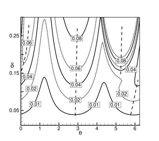
(b)

Figure 8: (a) Values of perturbation magnitude $J$ obtained at $t_{e}=2.5$ for the the evolutions of perturbations of the salinity-driven state in the tangent linear model and nonlinear model. The initial perturbations have the form $(T^{\prime}(0),S^{\prime}(0))=(\delta\cos\theta,\delta\sin\theta)$ with $\delta=0.2$ . And (b) the contour plot of $J(\theta,\delta)$, with contour interval of 0.02 from $J=0.02$ to $J=0.08$ (solid curve and dotted curve). The three group local maxima are indicated as the dashed curves .

(a)

(b)

Figure 9: Values of (a) perturbation growth $J/\delta$ and (b) flow stream function $\Psi$ along the trajectories computed with Conditional Nonlinear Optimal Perturbation (CNOP), initial conditions superposed on the salinity-driven state. The different curves are for different values of $\delta$.

(a)

(b)

Figure 10: Values of (a) perturbation growth $J$ and (b) flow stream function $\Psi$ along the trajectories computed with Conditional Nonlinear Optimal Perturbation (CNOP), initial conditions superposed on the thermally-driven state for different values of $\eta_{2}$.

Figure 11: The critical value of $\delta$ ($\delta_{c}$) versus the parameter controlling the thermally-driven state near the saddle-node bifurcation at $\eta_{2}=1.05$.

(a)

(b)

Figure 12: Values of (a) $J$ and (b) $\Psi$ along the trajectories computed with Conditional Nonlinear Optimal Perturbation (CNOP) initial conditions superposed on the salinity-driven state for different values of $\eta_{2}$.

Figure 13: The critical value of $\delta$ ($\delta_{c}$) versus the parameter controlling the salinity-driven state near the saddle-node bifurcation at $\eta_{2}=0.6$.

References

- Barclay et al. (1997) Barclay, A., P. E. Gill, and J. B. Rosen, 1997: SQP methods and their application to numerical optimal control. Technical Report Report NA 97-3, Dept of Mathematics, UCSD.
- Berloff and Meacham (1996) Berloff, P. S. and S. P. Meacham, 1996: Constructing fast-growing perturbations for the nonlinear regime. J. Atmos. Sci., 53, 2838–2851.
- Cessi (1994) Cessi, P., 1994: A simple box model of stochastically forced thermohaline flow. J. Phys. Oceanogr., 24, 1911–1920.
- Chen et al. (1997) Chen, Y. Q., S. D. Battisti, T. N. Palmer, J. Barsugli, and E. S. Sarachik, 1997: A study of the predictability of tropical pacific sst in a coupled atmosphere-ocean model using singular vector analysis: The role of the annual cycle and the enso cycle. Monthly Weather Review, 125, 831–845.
- Dijkstra (2000) Dijkstra, H. A., 2000: Nonlinear Physical Oceanography: A Dynamical Systems Approach to the Large Scale Ocean Circulation and El Niño. Kluwer Academic Publishers, Dordrecht, the Netherlands.
- Durbiano (2001) Durbiano, S., 2001: Vecteurs caracteristiques de modeles oceaniques pour la reduction d’ordre er assimilation de données. PhD thesis, Université Joseph Fourier, Grenoble, France.
- Gill and Saunders (1997) Gill, P. E. Murray, W. and M. A. Saunders, 1997: SNOPT: An sqp algorithm for large-scale constrained optimization. Technical Report Report NA 97-2, Dept of Mathematics, UCSD.
- Griffies and Tziperman (1995) Griffies, S. M. and E. Tziperman, 1995: A linear thermohaline oscillator driven by stochastic atmospheric forcing. J. Climate, 8, 2440–2453.
- Hasselmann (1976) Hasselmann, K., 1976: Stochastic climate models. I: Theory. Tellus, 28, 473–485.
- Knutti and Stocker (2002) Knutti, R. and T. F. Stocker, 2002: Limited predicability of future thermohaline circulation to an instability threshold. J. Climate, 15, 179–186.
- Liu and Nocedal (1989) Liu, D. C. and J. Nocedal, 1989: on the limited memory method for large scale optimization. Mathematical Programming, 45, 503–528.
- Manabe and Stouffer (1999) Manabe, S. and R. J. Stouffer, 1999: Are two modes of thermohaline circulation stable? Tellus, 51A, 400–411.
- Marotzke (1995) Marotzke, J., 1995: Analysis of thermohaline feedbacks. Technical Report No.39, Center for Global Change Science, M.I.T. Cambridge.
- McAvaney (2001) McAvaney, B., 2001: Chapter 8: Model evaluation. In Climate Change 2001: The Scientific Basis, Houghton, J. T., Ding, Y., Griggs, D. J., Noguer, M., van der Linden, P. J., and Xiaosu, D., editors. Cambridge University Press, 225-256.
- Mu et al. (2003) Mu, M., W. Duan, and B. Wang, 2003: Conditional nonlinear optimal perturbation and its applications. Nonlinear Proc. Geophysics, 10, 493–501.
- Mu and Duan (2003) Mu, M. and W. Duan, 2003: A new approach to study ENSO predictability: conditional nonlinear optimal perturbation. Chinese Science Bulletin, 48, 1045–1047.
- Mu and Wang (2001) Mu, M. and J. Wang, 2001: Nonlinear fastest growing perturbation and the first kind of predictability. Science in China, 44D, 1128–1139.
- Mu (2000) Mu, M., 2000: Nonlinear singular vectors and nonlinear singular values. Science in China, 43D, 375–385.
- Palmer (1995) Palmer, T. N., 1995: A nonlinear dynamical perspective on model error: A proposal for nonlocal stochastic-dynamic parameterisation in weather and climate prediction models. Quart. J. Roy. Meteor. Soc., 127, 279–304.
- Rahmstorf (1995) Rahmstorf, S., 1995: Bifurcations of the Atlantic thermohaline circulation in response to changes in the hydrological cycle. Nature, 378, 145–149.
- Stocker et al. (1992) Stocker, T. F., D. G. Wright, and L. A. Mysak, 1992: A zonally averaged, coupled ocean-atmosphere model for paleoclimate studies. J. Climate, 5, 773–797.
- Stommel (1961) Stommel, H., 1961: Thermohaline convection with two stable regimes of flow. Tellus, 2, 244–230.
- Thompson (1998) Thompson, C. J., 1998: Initial conditions for optimal growth in couple oceanatmosphere model of ENSO. J. Atmos. Sci., 55, 537–557.
- Timmermann and Lohmann (2000) Timmermann, A. and G. Lohmann, 2000: Noise-induced transitions in a simplified model of the thermohaline circulation. J. Phys. Oceanogr., 30, 1891–1900.
- Tziperman and Ioannou (2002) Tziperman, E. and P. J. Ioannou, 2002: Transient growth and optimal excitation of thermohaline variability. J. Phys. Oceanogr., 32, 3427–3435.
- Vélez-Belchí et al. (2001) Vélez-Belchí, P., A. Alvarez, P. Colet, J. Tintore, and R. L. Haney, 2001: Stochastic resonance in the thermohaline circulation. Geophys. Res. Letters, 28, 2053–2056.
- Xue and Zebiak (1997a) Xue, Y., M. A. C. and S. E. Zebiak, 1997a: Predictability of a coupled model of enso using singular vector analysis. part i: Optimal growth in seasonal background and enso cycles. Monthly Weather Review, 125, 2043 C2056.
- Xue and Zebiak (1997b) Xue, Y., M. A. C. and S. E. Zebiak, 1997b: Predictability of a coupled model of enso using singular vector analysis. part ii: optimal growth and forecast skill. Monthly Weather Review, 125, 2057 C2073.