Hydrodynamic and magnetohydrodynamic computations inside a rotating sphere

Abstract

Numerical solutions of the incompressible magnetohydrodynamic (MHD) equations are reported for the interior of a rotating, perfectly-conducting, rigid spherical shell that is insulator-coated on the inside. A previously-reported spectral method is used which relies on a Galerkin expansion in Chandrasekhar-Kendall vector eigenfunctions of the curl. The new ingredient in this set of computations is the rigid rotation of the sphere. After a few purely hydrodynamic examples are sampled (spin down, Ekman pumping, inertial waves), attention is focused on selective decay and the MHD dynamo problem. In dynamo runs, prescribed mechanical forcing excites a persistent velocity field, usually turbulent at modest Reynolds numbers, which in turn amplifies a small seed magnetic field that is introduced. A wide variety of dynamo activity is observed, all at unit magnetic Prandtl number. The code lacks the resolution to probe high Reynolds numbers, but nevertheless interesting dynamo regimes turn out to be plentiful in those parts of parameter space in which the code is accurate. The key control parameters seem to be mechanical and magnetic Reynolds numbers, the Rossby and Ekman numbers (which in our computations are varied mostly by varying the rate of rotation of the sphere) and the amount of mechanical helicity injected. Magnetic energy levels and magnetic dipole behavior are exhibited which fluctuate strongly on a time scale of a few eddy turnover times. These seem to stabilize as the rotation rate is increased until the limit of the code resolution is reached.

1 Introduction

In a previous paper, a spectral method for computing incompressible fluid and magnetohydrodynamic (MHD) behavior inside a sphere was introduced (Ref. [1], hereafter referred to as “MM”). The emphasis in MM was on accurate computation of global flow patterns throughout the full sphere (including the origin) with special attention to the computation of dynamo action, whereby the kinetic energy of a turbulent conducting fluid may give rise to macroscopic magnetic fields. The computations were limited to moderate Reynolds numbers, with boundary conditions in which the normal components of the velocity field, magnetic field, vorticity, and electric current density were required to vanish at a rigid, spherical, insulator-lined, perfectly-conducting shell, and the three components of the velocity and magnetic field were regular at the origin. The feature previously lacking that we wish to explore in the present paper is that of uniform rotation of the sphere. We postpone to the future the investigation of insulating spherical shells which permit the magnetic field to penetrate into a non-conducting region outside [2], though we remark later on some considerations relevant to this modification.

In Section 2, we formulate the equations to be solved for a uniform-density conducting fluid inside a sphere in a familiar set of dimensionless (“Alfvenic”) units. We refer to MM for background and such of the details as remain unchanged. The main changes reported here are: (1) the introduction of a Coriolis term in the equation of motion (the centrifugal term may be absorbed in the pressure for incompressible flow); and (2) the velocity field ${\bf v}$ (instead of the vorticity $\omega$) and magnetic field ${\bf B}$ are expanded in orthonormal Chandrasekhar-Kendall (“C-K”) vector eigenfunctions of the curl [3, 4, 5, 6, 1]. The physical situation being simulated is again a perfectly conducting, mechanically impenetrable sphere coated on the inside with a thin layer of insulator, but now viewed from a coordinate system that is regarded as rigidly rotating with the bounding spherical shell. Unsurprisingly, the dynamical phenomena resulting are markedly different from, and richer than, they were in the case without rotation.

Section 3 describes the results of some purely hydrodynamic runs (the code may be readily converted into a Navier-Stokes code by simply deleting the terms associated with the magnetic field). Included are examples [7, 8] of: (i) spin down, or decay of relatively rotating kinetic energy due to the action of viscosity; (ii) Ekman pumping with flow patterns that result from rotating boundaries; (iii) internal waves, three-dimensional relatives of meteorological Rossby waves, that depend on the stabilization introduced by rotation for their oscillatory features; and (iv) some mechanically-forced runs with a finite angle between the symmetry axis of the forcing and the axis of rotation. This fourth case results in columnar vortices due to the effect of rotation [8, 9] (note convection is absent in our present formulation).

Section 4 proceeds to a consideration of the MHD case with an emphasis on selective decay and the kinds of dynamo behavior we have been able to resolve. The spectral method we use involves inherently less resolution than some other methods in use, and we have been careful to study parameter regimes only where we can resolve the relevant length scales. Selective decay is observed to be somewhat arrested as the rotation rate is increased. A pleasant surprise has been the wide variety of dynamo behavior we have been able to resolve without the need to reach parameter regimes regarded as realistic for planetary dynamos [10, 11, 9, 12, 13, 2]. In the summary, Section 5, we describe briefly some plans we have for improving the resolution of the code by some pseudo-spectral modifications and some intended future diversification of the boundary conditions.

2 Computational method

We begin from the magnetohydrodynamic (MHD) equation of motion in a rotating coordinate frame [14, 2],

$$\frac{\partial{\bf v}}{\partial t}={\bf v}\times\mbox{\boldmath$\omega$}+{\bf j}\times{\bf B}-\nabla\left({\mathcal{P}}+\frac{v^{2}}{2}\right)-2\mbox{\boldmath$\Omega$}\times{\bf v}+\nu\nabla^{2}{\bf v}+{\bf f},$$ (1)

and the MHD induction equation,

$$\frac{\partial{\bf B}}{\partial t}=\nabla\times\left({\bf v}\times{\bf B}\right)+\eta\nabla^{2}{\bf B}.$$ (2)

In the dimensionless Alfvenic units [1], ${\bf v}$ is the vector velocity field, ${\bf B}$ is the magnetic induction, $\mbox{\boldmath$\omega$}=\nabla\times{\bf v}$ is the vorticity, and ${\bf j}=\nabla\times{\bf B}$ is the electric current density. The generalized pressure is ${\mathcal{P}}$. The dimensionless viscosity, which, in the dimensionless variables, can be interpreted as the reciprocal of a mechanical Reynolds number, is $\nu$, and the magnetic diffusivity, which can be interpreted as the reciprocal of a magnetic Reynolds number, is $\eta$. The vector field ${\bf f}$ is a solenoidal, externally-applied forcing field which is intended to mimic the presence of mechanical sources of excitation of ${\bf v}$. Equations (1) and (2) are to be supplemented by the requirements that the divergences of both ${\bf v}$ and ${\bf B}$ must vanish everywhere. Dropping equation (2) and the terms in equation (1) containing ${\bf j}$ and ${\bf B}$ leaves the forced Navier-Stokes equation, and dropping ${\bf f}$ leaves the unforced version of Navier-Stokes. $\Omega$ is the (constant) rotation speed of the coordinate system, understood to be attached to a rotating spherical shell that constitutes the boundary and is both mechanically impenetrable and perfectly conducting, with a thin layer of insulator on the inside surface.

The non-trivial boundary conditions imposed are that the normal components of ${\bf v}$, ${\bf B}$, ${\bf j}$, and $\omega$ shall all vanish at the radius of a unit sphere centered at the origin. The three components of the fields ${\bf v}$ and ${\bf B}$ are also required to be regular at the origin. The vanishing of the normal components of ${\bf v}$ and $\omega$ at the surface of the unit sphere are implied by, but do not imply, no-slip boundary conditions at that radius. Going further with an attempt to implement fully a set of no-slip boundary conditions raises unresolved paradoxes with respect to the pressure determination which we prefer not to confront here (see Refs. [15, 16, 1] for a discussion of these), believing that their seriousness and intractability require consideration in the context of simpler situations than the present one.

The spectral technique implemented involves expanding ${\bf v}$ and ${\bf B}$ in terms of C-K functions (defined below):

$${\bf v}({\bf r},t)=\sum_{qlm}\xi^{v}_{qlm}(t)\,{\bf J}_{qlm}({\bf r}),$$ (3)

and

$${\bf B}({\bf r},t)=\sum_{qlm}\xi^{B}_{qlm}(t)\,{\bf J}_{qlm}({\bf r}).$$ (4)

The C-K functions [3, 4, 5, 6, 1] ${\bf J}_{i}$ are defined by

$${\bf J}_{i}=\lambda\nabla\times{\bf r}\psi_{i}+\nabla\times\left(\nabla\times{\bf r}\psi_{i}\right),$$ (5)

where we work with a set of spherical orthonormal unit vectors $(\hat{r},\hat{\theta},\hat{\phi})$ and the scalar function $\psi_{i}$ is a solution of the Helmholtz equation, $(\nabla^{2}+\lambda^{2})\psi_{i}=0$. The explicit form of $\psi_{i}$ is

$$\psi_{i}(r,\theta,\phi)=C_{ql}\,j_{l}(|\lambda_{ql}|r)Y_{lm}(\theta,\phi),$$ (6)

where $j_{l}(|\lambda_{ql}|r)$ is a spherical Bessel function of the first kind which vanishes at $r=1$ and $Y_{lm}(\theta,\phi)$ is a spherical harmonic in the polar angle $\theta$ and the azimuthal angle $\phi$. The subindex $i$ is a shorthand notation for the three indices $(q,l,m)$, where $q$ indexes the successive values of $\lambda$ that make $j_{l}$ vanish at $r=1$ for each value of $l$; $q=1,2,3,\dots$ corresponds to the positive values of $\lambda$, and $q=-1,-2,-3,\dots$ indexes the negative values; finally $l=1,2,3,\dots$ and $m$ runs in integer steps from $-l$ to $+l$. The vectors ${\bf J}_{i}$ satisfy

$$\nabla\times{\bf J}_{i}=\lambda_{i}{\bf J}_{i},$$ (7)

and with the proper normalization constants are an orthonormal set that has been shown to be complete [6]. The integral relation expressing the orthogonality of the ${\bf J}_{i}$ is:

$$\int{\bf J}_{qlm}\cdot{\bf J}_{q^{\prime},l^{\prime},m^{\prime}}^{*}dV=\delta_{q,q^{\prime}}\delta_{l,l^{\prime}}\delta_{m,m^{\prime}},$$ (8)

where the asterisk denotes complex conjugate, and with the normalization constants given by:

$$C_{ql}=\left|\lambda_{ql}\,j_{l+1}(|\lambda_{ql}|)\right|^{-1}\left[l(l+1)\right]^{-1/2}.$$ (9)

The scheme for solving equations (1) and (2) is conceptually simple. We substitute the expansions (3) and (4) into equations (1) and (2), utilize the fact that the ${\bf J}_{i}$ are eigenfunctions of the curl, and then take inner products one at a time with the individual ${\bf J}_{i}$. Their orthogonality enables us to pick off expressions for the time derivatives of the time dependent expansion coefficients $\xi_{i}^{v}$ and $\xi_{i}^{B}$, and equations (1) and (2) are thereby converted into a set of ordinary differential equations for the expansion coefficients. These appear as

$$\frac{\partial\xi^{v}_{i}}{\partial t}=\sum_{j,k}A^{i}_{jk}\left(\xi^{v}_{j}\xi^{v}_{k}-\xi^{B}_{j}\xi^{B}_{k}\right)+2\sum_{j}\mbox{\boldmath$\Omega$}\cdot{\bf O}^{i}_{j}-\nu\lambda_{i}^{2}\xi^{v}_{i}+\xi^{f}_{i},$$ (10)

and

$$\frac{\partial\xi^{B}_{i}}{\partial t}=\sum_{j,k}B^{i}_{jk}\xi^{v}_{j}\xi^{B}_{k}-\eta\lambda_{i}^{2}\xi^{B}_{i},$$ (11)

with the coupling coefficients defined as

$$A^{i}_{jk}=\lambda_{k}I^{i}_{jk},\;\;\;\;\;B^{i}_{jk}=\lambda_{i}I^{i}_{jk},$$ (12)

$$I^{i}_{jk}=\int{\bf J}_{i}^{*}\cdot{\bf J}_{j}\times{\bf J}_{k}dV,\;\;\;\;\;{\bf O}^{i}_{j}=\int{\bf J}_{i}^{*}\times{\bf J}_{j}dV.$$ (13)

Figure 1: (a) Time histories of the decay of mechanical energy for four hydrodynamic runs (H1 to H4) with identical initial velocity fields but different rotation rates $\Omega$. (b) Decay rates vs. the square root of $\Omega$ for the same four runs.

The infinite set of ordinary differential equations is truncated at some level above maximum values of $|q|$ and $l$, in the usual manner of a Galerkin approximation [17]. The evaluation of equations (10) and (11) and the storage of the resulting arrays of coupling coefficients in tables, are the most demanding numerical tasks of the problem. Once available, they do not have to be recomputed, and provide a method for verifying the ideal quadratic conservation laws with high accuracy [1]. Also, since the method is purely spectral and fields are only computed in real space for visualization purposes, there is no numerical singularity in the center of the sphere.

The main drawback of the scheme, as with any wholly spectral one, is that the convolution sums in equations (10) and (11) grow rapidly with increasing maximum values of $|q|$ and $l$, and limit the resolution when compared to pseudospectral computations utilizing fast transforms (in practice, a resolution of $\max\{|q|\}=\max\{l\}=9$ was used in all the runs). This limits us to modest Reynolds numbers (all our computations reported here have limited themselves to resolvable Reynolds numbers). Future plans include pseudospectral modifications to the evaluation of at least the angular parts of the nonlinear terms in equations (1) and (2), as will be mentioned again in the final summary (Section 5).

3 Hydrodynamic examples

Some neutral-fluid effects (good introductions to all of which may be found in Refs. [7, 8]) are treated first before proceeding to MHD. It is worth noticing here that although our boundary conditions are implied by, but do not imply no-slip velocities, several qualitative and some quantitative agreements are observed with previous experiments and theory. First we study simple problems in which initially relatively rotating fluids adjust themselves to rigid rotation with the spherical shell. We study these decays as functions of the rotation rate $\Omega$. The prediction [7] is that the decay of the non-rigid body components should be exponential, with a decay rate that varies as $\Omega^{1/2}$. Figure 1(a) shows the time histories of the decay of mechanical energy for four runs with identical initial velocity fields limited to a few random low mode numbers (large spatial scales). The runs are delineated as runs H1, H2, H3, and H4. Specifically, we have as initial conditions a random superposition of modes with $|q|=1,2$, $l=1,2$, and all allowed values of $m$, with viscosity $\nu=0.01$ and values of $\Omega$ of $0$, $1$, $4$, and $10$ respectively. Each curve is approximately exponential, and when they are fitted with exponentials, the decay rates plotted vs. the square root of $\Omega$ appear as in Figure 1(b), and are adjudged to be in satisfactory agreement with theory [7]. The nonlinearities excite smaller spatial scales, and the decay process is progressively enhanced by increasing the rotation rate.

Figure 2: (a) Enstrophy for runs H1 to H4 as a function of time (same labels as in Figure 1). (b) Energy spectra at $t=1$ for the same runs, and (c) energy spectra at $t=6$. In all cases, solid lines are for $\Omega=0$, dotted lines for $\Omega=1$, dashed lines for $\Omega=4$, and dash-dotted lines for $\Omega=10$.

A second feature of rotating spherical flows observed in our code is the development of Ekman-like layers and the action of Ekman pumping [7, 8] (see also [18] for a detailed study in rotating spherical shells). The flow patterns are characterized by the development of interior vortical flows with some symmetries, and thin layers that separate the large vortices and also lie along the wall boundary layers. These have a characteristic thickness of the order of $\delta\sim E_{K}^{1/2}R$, where $R=1$ is the radius of the sphere, and the Ekman number is $E_{K}=\nu\Omega^{-1}L^{-2}$, with $L$ a characteristic scale of the flow. The ability of the code to compute these layers is limited by its resolution. Realistic values of the Ekman number are, for planetary core regimes [14, 9, 2], beyond our range. In all the runs presented here we will limit ourselves to cases where $\delta$ can be properly resolved with the number of modes used in the simulations. The presence of the Ekman layers is concomitant with the development of smaller spatial scales and hence of more rapid dissipation. Figure 2 illustrates this fact. Figure 2(a) is the integrated squared vorticity, or enstrophy, for the four runs whose decay has just been seen to be exponential. The largest rotation rate corresponds to the curve with the highest early peak in enstrophy spectrum, the second highest with the second largest, and so on. Figure 2(b) shows the energy spectra at $t=1$ for the four runs and Figure 2(c) shows the same energy spectra at $t=6$. In every case, the flatter spectra, and hence the shorter wavelength dominances, correspond to the higher values of $\Omega$. This is the result of the formation of a thinner boundary layer as $\Omega$ is increased.

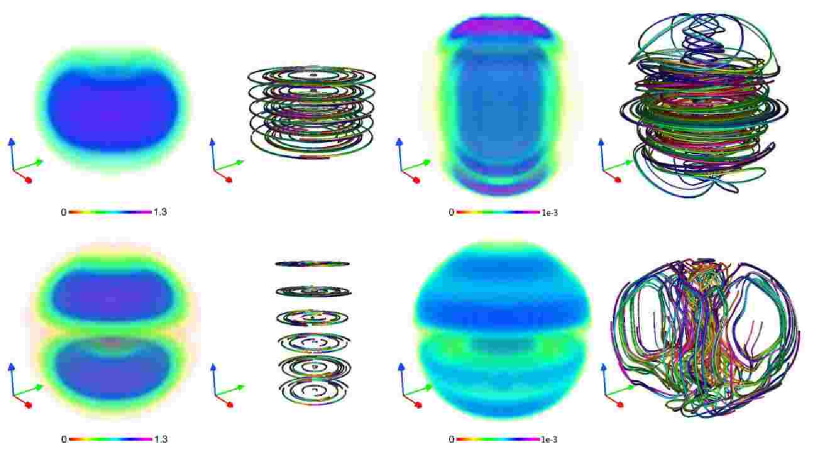
Figure 3: Above: Mechanical energy density and velocity field lines in run E1, at $t=0$ (left) and at $t=6$ (right). Below: idem for run E2. For convenience, energies and field lines are always shown in pairs, with energy densities on the left and field lines on the right. The field lines change color according to the distance integrated from the initial point, from red to yellow, blue, and magenta. The red, green, and blue arrows indicate respectively the $x$, $y$, and $z$ axis. $\Omega$ is in the $z$ direction. In both cases, the energy density is symmetric with respect to the equator, while the flow itself is antisymmetric in run E1 (above).

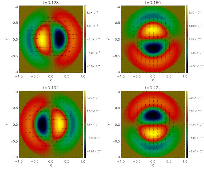
Figure 4: Equatorial cross section of the velocity field for an inertial wave in the rotating sphere. The reference frame is fixed to the sphere. $\Omega$ is in the $z$ direction. The axial velocity is indicated by the colors, while the radial and azimuthal velocities are indicated by the arrows. For this mode, the frequency is $\varpi\approx 49$.

The range of Ekman layer behavior we have been able to observe is very wide. We show in Figure 3 the results of two simulations (labeled E1 and E2) with initially random axisymmetric ($m=0$) velocity fields which are purely azimuthal. For both runs, the initial velocity is proportional to the difference between ${\bf J}_{q,l,0}$ and ${\bf J}_{-q,l,0}$, which has only an azimuthal component. For run E1, $q=1$ and $l=1$, and for run E2, $q=1$ and $l=2$. Both runs have $\nu=0.01$ and $\Omega=10$. The time evolution of the runs is similar to the evolution displayed in Figures 1 and 2. However, the axisymmetric initial conditions in runs E1 and E2 make visualization of flow patters easier. Figure 3 shows the initial and late-time flow patterns for these runs, using the VAPOR graphics package [19] that will be repeatedly used throughout this paper for graphical demonstrations. The rotation generates poloidal components of the velocity field fast, and at late times different patterns are observed depending on the initial value of $l$. In run E1, at late times the flow displays a poloidal circulation on top of the initial toroidal field: the flow is directed towards the center of the sphere along the axis of rotation, and a return flow is observed in both hemispheres close to the wall. In other words, the flow can be described as the superposition of a toroidal differential rotation and a poloidal meridional circulation. This circulation is radially outward in the meridional plane, directed towards the poles close to the wall, and redirected toward the equatorial plane again as the flow gets close to the poles. Both hemispheres show the same pattern. In run E2 the pattern is more complex, and vertical velocities are observed in the vicinity of the axis of rotation, while high and at intermediate latitudes a poloidal circulation is generated.

Figure 5: (a) Magnetic energy $E_{M}$ (solid line), kinetic energy $E_{V}$ (dotted line), and magnetic helicity $H_{M}$ (dashed line) in the selective decay run S1. (b) Same quantities for run S2. The two power laws are indicated in the figures only as a reference.

As a third hydrodynamic test of the code we demonstrate inertial wave motion in the small-amplitude limit. Equations (10) and (11) can be linearized in powers of a small departure from a uniform rotation velocity; then solutions can be sought which vary with time as $e^{i\varpi t}$. The resulting linear homogeneous algebraic system can be solved in a Galerkin approximation by expanding the velocity and vorticity in the C-K functions. An anti-Hermitian matrix results whose eigenfunctions can be found numerically and whose corresponding eigenvalues $i\varpi$ may be computed numerically in the process. Then any one of the oscillatory modes can be loaded numerically into the ideal version of the code and run with the overall amplitudes chosen to be very small. The time evolution is accurately predicted by the computation of the single modes, which are standing waves. Figure 4 shows four equatorial cross-sections of the sphere at different times with the axial velocity indicated by the color codes, and the radial and azimuthal velocities indicated by arrows ($\Omega=10$ in this run). The times are chosen to be one quarter-period apart. The oscillation frequency $\varpi$ for the particular mode shown as obtained from the eigenvalue problem is in good agreement with the results obtained from the fully non-linear code ($\varpi\approx 49$).

In forced hydrodynamic simulations in the presence of strong rotation, we also observe the development of columnar structures in the flow, aligned with the axis of rotation. The discussion of these simulations will be left for the next section, where the connection between these columns and dynamo action will be considered.

4 MHD and the dynamo

4.1 Selective decay in the sphere

Figure 6: Relative helicity $H_{M}/E_{M}$ in selective decay runs S1 (solid) and S2 (dashed).

Before passing to a discussion of the mechanically driven spherical dynamo, we present first the results of two tests of three-dimensional MHD “selective decay” as affected by the presence of rotation. Selective decay is a familiar turbulent decay process, usually incompressible, long studied in periodic geometry [20, 21, 22], wherein one ideal invariant is cascaded to short wavelengths and dissipated while another remains locked into long wavelengths and is approximately conserved. The phenomenon, closely connected with inverse cascade processes for driven systems, leads toward a state in which the ratio of the two ideal invariants involved is minimized and which therefore is accessible to variational methods. In 3D MHD, a quantity that may be preferentially dissipated is the total energy $E=E_{V}+E_{M}$ (kinetic plus magnetic) while magnetic helicity $H_{M}$ may be approximately conserved. Under other circumstances, energy may be dissipated while cross helicity $K$ is approximately conserved, leading to the phenomenon of “dynamic alignment,” [23, 24, 25] in which the velocity field and magnetic fields are highly correlated. The definitions of $H_{M}$ and $K$ are

$$H_{M}=\frac{1}{2}\int{\bf A}\cdot{\bf B}dV,$$ (14)

$$K=\frac{1}{2}\int{\bf u}\cdot{\bf B}dV,$$ (15)

where ${\bf A}$ is the vector potential whose curl is ${\bf B}$, and the integrals run over the entire volume of the fluid. What we are interested in demonstrating here is the effect that rotation has on the development of the selective decay of total energy relative to magnetic helicity inside a sphere. It will be useful for these and other purposes, to have a definition of the magnetic dipole moment:

$$\mbox{\boldmath$\mu$}=\frac{1}{2}\int{\bf r}\times{\bf j}\,dV\,.$$ (16)

which is seen to be readily expressible in terms of the expansion coefficients for ${\bf B}$ [1].

Figure 7: (a) Trace of the dipole moment on the surface of the unit sphere (above) and amplitude of the dipole moment as a function of time (below) for the selective decay run S1. (b) Same quantities for run S2.

The initially excited modes for the two runs we will present (“S1” and “S2”) are those for $q=\pm 3$, $l=3$, and all possible values of $m$. The initial values chosen for the expansion coefficients are:

$$\xi^{v}_{\pm 3,3,0}=-u_{0},\;\;\xi^{v}_{\pm 3,3,0<m\leq 3}=u_{0}(1+i),$$ (17)

$$\xi^{B}_{3,3,0}=\frac{10}{6}\xi^{B}_{-3,3,0}=b_{0},\;\;\xi^{B}_{3,3,0<m\leq 3}=\frac{10}{6}\xi^{B}_{-3,3,0<m\leq 3}=b_{0}(1-i),$$ (18)

with $u_{0}$ and $b_{0}$ chosen so that at $t=0$, the magnetic and kinetic energies are $E_{M}=E_{V}\approx 0.5$, $K=0$, and $H_{M}\approx 0.034$. Some helicity cancellation occurs because of the two signs of $\lambda$ (or $q$). As a comparison, note that for the $q=3$, $l=3$ mode alone, $H_{M}/E_{M}$ is no more than about $0.072$ (this is the maximum value of $|H_{M}/E_{M}|$ if only modes with $|q|=3$, $l=3$, and one sign of $\lambda$ are excited). In both runs, the magnetic diffusivity and kinematic viscosity are $\nu=\eta=0.006$; the Reynolds numbers are $R_{e}\approx R_{m}\approx 170$, based on the radius of the sphere. The two runs differ by the values of $\Omega$ chosen, which are $2$ and $12$, respectively. These mean that the Rossby and Ekman numbers of the two runs are, respectively, $R_{O}=U(\Omega R)^{-1}=0.5$, $E_{K}=0.003$ for S1 and $R_{O}=0.083$, $E_{K}=0.0005$ for S2. The decay of magnetic energy, kinetic energy, and magnetic helicity for Runs S1 and S2 are shown in Figure 5. The behavior in Run S1 is not significantly different from the non-rotating case [1]. Note that in both runs, the kinetic energy at late times is negligible, and that magnetic and kinetic energies decay faster than the magnetic helicity. However, the decay of all these quantities in S2 seems to be faster than in S1.

The relative helicity, $H_{M}/E_{M}$, is shown for Runs S1 and S2 in Figure 6. It will be seen that the increased rate of rotation in S2 has somewhat arrested the selective decay, for reasons not totally understood. It may be that the rotation has resulted in sufficient two-dimensionalization of the flow [7, 8, 9] that the inherently three dimensional nature of the selective decay has been compromised. But from Figure 6 it can also be seen that the ratio of $H_{M}$ to $E_{M}$ has approached reasonably closely to its maximal value of $\min^{-1}\{|\lambda_{ql}|\}\approx 0.22$ (the maximum value of $|H_{M}/E_{M}|$ when only modes with $|q|=1$, $l=1$, and one sign of $\lambda$ are excited). The maximal value would indicate a total disappearance of the non-rotational kinetic energy (i.e., a rigid rotation), and all the magnetic energy in the largest-scale modes (smallest $|\lambda|$) allowed by the boundary conditions: a magnetized, “frozen” condition.

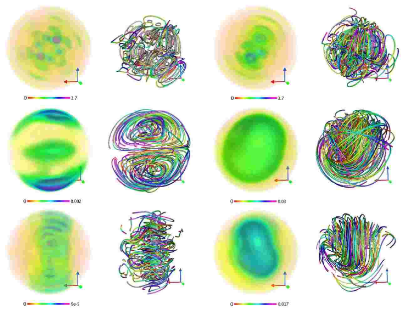
Figure 8: Above: kinetic energy density and velocity field lines (left) and magnetic energy density and magnetic field lines (right) in the initial conditions of selective decay runs S1 and S2. Middle: same fields at $t=14$ in run S1. Below: same fields at $t=14$ in run S2. Colors and labels are as in Figure 3.

The behavior of the dipole moment for the two runs is shown in Figure 7. The solid lines are the traces of the projected direction of the dipole moment on the surface of the sphere as functions of the time, and the orientation is such that the axis of rotation points upward. In the lower parts of these two figures, the magnitude of the dipole moment is plotted vs. time. In both cases, it will be seen that the dipole’s orientation initially wanders erratically near its initial position, and finally ends at a “mid-latitude” direction not far from where it began. This was something of a surprise to us, since we had expected it to line up with the axis of rotation or at least close to it. Figure 8 shows VAPOR plots with the energy densities, velocity and magnetic field line structure for the initial conditions in Runs S1 and S2, as well as the late stages of both runs ($t=14$) when the selective decay process has saturated and all the nonlinear terms are small, preventing any further evolution of the system except for dissipation. For strong rotation (run S2), the velocity field is quasi-two dimensional and develops column-like structures at late times, while the magnetic field is highly anisotropic (although the dipole moment is not aligned with the axis of rotation). Note magnetic field lines in this case are aligned with the $z$ axis (the axis of rotation), and velocity field lines are mostly toroidal. Actually, the ratio $|v_{\phi}/v_{z}|$ at $t=14$ averaged over the whole volume for this run at $t=14$ is $\approx 13$.

Table 1: Dynamo runs: $q$ and $l$ give the scales where mechanical energy is injected by the forcing, $\Omega$ is the rotation rate, and $\nu$ and $\eta$ are respectively the kinematic viscosity and magnetic diffusivity. “Helical” indicates whether the forcing injects mechanical helicity, and “Axisym.” indicates whether the forcing is axisymmetric. $\alpha$ is the angle between $\Omega$ and the $z$-axis (the axis of symmetry in axisymmetric forcings). Finally, $R_{O}$, $E_{K}$, and $R_{e}$ are respectively the Rossby, Ekman, and Reynolds numbers, all based on the radius of the sphere. A resolution of $\max\{|q|\}=\max\{l\}=9$ was used in all the runs.

• Runs	$q$	$l$	$\Omega$	$\nu=\eta$	Helical	Axisym.	$\alpha$	$R_{O}$	$E_{K}$	$R_{e}$
  D1	1	1	2	$2\times 10^{-3}$	No	Yes	$30^{\circ}$	$0.5$	$1\times 10^{-3}$	$500$
  D2	2	2	2	$2\times 10^{-3}$	No	Yes	$30^{\circ}$	$0.5$	$1\times 10^{-3}$	$500$
  D3	3	3	2	$2\times 10^{-3}$	No	Yes	$30^{\circ}$	$0.5$	$1\times 10^{-3}$	$500$
  D4	3	3	4	$2\times 10^{-3}$	No	Yes	$30^{\circ}$	$0.25$	$5\times 10^{-4}$	$500$
  D5	3	3	8	$2\times 10^{-3}$	No	Yes	$30^{\circ}$	$0.125$	$2.5\times 10^{-4}$	$500$
  D6	3	3	8	$4\times 10^{-3}$	No	Yes	$30^{\circ}$	$0.125$	$5\times 10^{-4}$	$250$
  D7	3	3	16	$4\times 10^{-3}$	No	Yes	$30^{\circ}$	$0.0625$	$2.5\times 10^{-4}$	$250$
  D8	3	3	8	$2\times 10^{-3}$	No	Yes	$30^{\circ}$	$0.125$	$2.5\times 10^{-4}$	$500$
  D9	3	3	16	$4\times 10^{-3}$	No	Yes	$20^{\circ}$	$0.125$	$5\times 10^{-4}$	$250$
  D10	3	3	16	$4\times 10^{-3}$	No	No	$0^{\circ}$	$0.125$	$5\times 10^{-4}$	$250$
  D11	3	3	16	$4\times 10^{-3}$	Yes	No	$0^{\circ}$	$0.125$	$5\times 10^{-4}$	$250$
  D12	3	3	16	$4\times 10^{-3}$	Yes	No	$90^{\circ}$	$0.125$	$5\times 10^{-4}$	$250$

4.2 Dynamos

We turn now to the case of the forced spherical dynamo computations, in which specified non-zero forcing functions ${\bf f}$ are added to the right hand side of equation (1) or (10) to provide a persistently-active, non-decaying velocity field. After a purely hydrodynamic run to reach a statistically steady state, very small magnetic fields are introduced to see if the velocity fields will cause them to amplify, and attention focuses on questions like the orientation of the resulting magnetic dipole moment relative to the axis of rotation and the dipole moment’s magnitude. We are also interested in the kinetic and magnetic energy spectra that result, and how the eponymous dimensionless numbers of the rotating fluid (Reynolds, magnetic Reynolds, Rossby, Ekman) influence the magnetic quantities. These appear to be essential control parameters of the problem. The range of possibilities is clearly very wide, and we have not begun to explore the entire space of possible parameters. Rather, we content ourselves with showing samples of different behavior that have emerged for different combinations that lead to regimes which the code will resolve satisfactorily. Our efforts should not be compared with explorations of the space of parameters in realistic geodynamo simulations (see e.g. [26]) but rather as an extension of dynamo simulations of incompressible MHD flows (often done using periodic boundary conditions [27, 28, 29, 30]) to include the effect of boundaries and rotation.

Several of the forcing functions used in the runs we will display are axisymmetric, but their axes of symmetry are not aligned with the axis of rotation. The resulting overall asymmetry quickly excites all the available retained modes, to some degree. The general form of the axisymmetric forcing function used is

$${\bf f}=\sum_{ql}\xi^{f}_{q,l,0}\left(A{\bf J}_{q,l,0}-B{\bf J}_{-q,l,0}\right).$$ (19)

For any value of $A$ and $B$, this superposition of C-K functions gives an axisymmetric forcing ${\bf f}$. For $A=B=1$, there will be no net helicity involved in the forcing (the curl of ${\bf f}$ is perpendicular to ${\bf f}$), and the only non-vanishing component of velocity that is forced is the $\phi$ component (the azimuthal component with respect to the axis of symmetry of the forcing, the $z$ axis). This forcing can be considered as a simple differential rotation, where the number of nodes in $v_{\phi}(r,\theta)$ is controlled by the values of $q$ and $l$. The axis of rotation is typically oriented at some specified angle $\alpha$ (often $30^{\circ}$) to the forcing function’s axis of symmetry (the polar axis, in spherical coordinates). Thus the rotational motion and the forcing have no shared symmetry, and the resulting mechanical motion is totally asymmetrical.

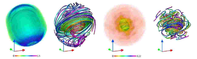
Figure 9: Left: kinetic energy density and velocity field lines at late times in run D1, when the dynamo has saturated. Right: magnetic energy density and magnetic field lines at the same time. Colors and labels are as in Figure 3.

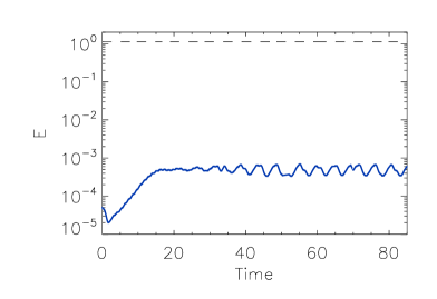
Figure 10: Left: kinetic (dashed black line) and magnetic (solid blue line) energy as a function of time in run D1. Right: cosine of the angle between $\Omega$ and $\mu$ in the same run.

Non-axisymmetric forcing functions are obtained by superposing C-K modes with $m\neq 0$, i.e.

$${\bf f}=\sum_{qlm}\xi^{f}_{qlm}{\bf J}_{qlm},$$ (20)

and when $\xi^{f}_{qlm}=\xi^{f}_{-q,l,m}$ the forcing is non-helical. In any other case the curl of ${\bf f}$ has a projection into ${\bf f}$, and the forcing injects mechanical helicity into the flow.

In an effort to systematize the runs we have done and the reasons we have done them, we have assembled the important parameters for the dynamo runs (labeled D1 through D12) in Table 1. Listed in Table 1 are: the $q$ and $l$ values where the forcing was concentrated (determining its characteristic length scale); the rigid rotation rate; the kinematic viscosity (reciprocal Reynolds number, if the kinetic energy is close to unity) and magnetic diffusivity (this study is restricted to the magnetic Prandtl number $P_{M}=\nu/\eta=1$ case); an indication of whether the forcing was axisymmetric or not; the angle between the axis of rotation and the axis of symmetry of the forcing, when the forcing function has an internal symmetry; the Rossby and Ekman numbers of the flow into which the seed magnetic field is introduced; and whether or not the forcing injected net mechanical helicity.

It is perhaps worthwhile to say a word about the motivation for the progression of runs shown in Table 1. The first remark is that it seems to be relatively easy to excite a dynamo and generate a dipole moment, but relatively difficult to generate one that behaves according to our predispositions and hopes: a dipole moment with some alignment with the axis of rotation, and that reverses periodically or randomly with long times between reversals (compared with the turbulent turnover time). We have found wild oscillations in both magnitude and direction that seem to decrease with decreasing Rossby and Ekman numbers. Since the Reynolds numbers are limited by the resolution, the principal means of decreasing both the Rossby and Ekman numbers is by increasing the rotation rate $\Omega$. This, however, eventually decreases the thickness of the boundary layer below the resolution of the code, and beyond that point, the accuracy of the computations becomes suspect. The lowest Rossby and Ekman numbers that appear in the entries of Table 1 represent those below which the resolution limitations are encountered. It will be seen below that as we progress toward them, the dipolar behavior looks gradually more like what we might expect, the dipole moment gets stronger and more aligned with the axis of rotation, and the time between reversals gets larger.

We begin by showing some results for a weak dynamo situation, Run D1, where the magnetic energy $E_{M}$ remains always much smaller than the kinetic energy $E_{V}$. In the forcing function (19), the driven modes have $q=l=1$, $A=B=1$, $\nu=\eta=0.002$, $\alpha=30^{\circ}$, and $\Omega=2$. The amplitude of the forced modes is $|\xi^{f}_{q,l,0}|=0.4$. The two Reynolds numbers, $R_{e}$ and $R_{m}$, based on the measured r.m.s. velocity before the magnetic seed is introduced and the radius of the sphere, are both about 500. The Rossby number is $R_{O}=0.5$, and the Ekman number also based on the radius of the sphere is $E_{K}=1\times 10^{-3}$. Figure 9 shows the streamlines of the flow, magnetic field lines, and the energy densities at late times, once the dipole is established ($t\approx 80$). In the steady state, the magnetic dipole moment $|\mbox{\boldmath$\mu$}|$ is of the order of $0.001$ and the ratio of magnetic to kinetic energies is $E_{M}/E_{V}\approx 0.0005$. The magnetic energy rises to a characteristic value and oscillates somewhat irregularly as shown in Figure 10, while the cosine of $\gamma$ (the angle between the axis of rotation and the orientation of $\mu$) oscillates with roughly the same periodicity (see also Figure 10) with almost a $180^{\circ}$ variation in some cases, and with an average orientation almost perpendicular to $\Omega$. In this weak case D1, the hydrodynamic flow remains laminar, stable, and almost time independent.

Figure 11: (a) Magnetic energy in dynamo runs D1 (solid), D2 (dotted), D3 (dashed), D4 (dash-dotted) and D5 (dash-triple dotted). (b) Magnetic energy spectrum for the same runs at late times, after non-linear saturation of the dynamo takes place. The arrows on top indicate the scale where mechanical energy is injected in each run; from left to right: D1, D2, and D3-D5. The magnetic energy spectrum corresponding to Run D1 has been multiplied by a factor of 100.

The global evolution of the system is similar to what we will show in the remaining runs. Once the magnetic field is introduced at $t=0$, and if $R_{m}$ is large enough, the magnetic field is amplified exponentially (this stage is often called the “kinematic dynamo” regime) until the Lorentz force modifies the flow and non-linear saturation is reached. At late times, an MHD state is reached in which magnetic energy is sustained against Ohmic dissipation by dynamo action. In run D1, the flow is reminiscent of the hydrodynamic flow previously described in Figure 3. Although the forcing is axisymmetric and purely toroidal, rotation generates a poloidal circulation and as a result the flow points outwards in the equatorial plane, and inwards along the axis of rotation. Each hemisphere has mechanical helicity of opposite signs, while the net mechanical helicity of the system fluctuates around zero. The magnetic field seems to be sustained by an $\alpha$-$\Omega$ mechanism, where the differential rotation is sustained by the mechanical forcing and the $\alpha$-effect is given by the Ekman-like circulation. Magnetic energy is concentrated in the center of the sphere, where the flow has a stagnation point.

Figure 12: Left: (a) Trace of the dipole moment on the surface of the unit sphere (above), amplitude of the dipole moment (middle), and cosine of the angle between the dipole moment and the axis of rotation as a function of time, for run D3. (b) Same quantities for run D5. (c) Same quantities for run D7.

A considerably stronger dynamo than D1 is represented in Run D2, where in the excitation function (19) we choose $q=l=2$ and $|\xi^{f}_{q,l,0}|=1.1$. Again, $A=B=1$, $\nu=\eta=0.002$, and $\Omega=2$. The magnetic moment rises from zero, and attains a typical magnitude of $|\mbox{\boldmath$\mu$}|\approx 0.5$, about 100 times larger than in D1. The Reynolds numbers are $R_{e}=R_{m}\approx 500$, and the ratio of magnetic to kinetic energy oscillates around $0.15$. The cosine of $\gamma$ (the angle between $\mu$ and $\Omega$) oscillates wildly in time, and the orientation of the dipole shows no preferred direction. The only difference between run D1 and D2 is the change in the forcing scale, and the result seems to indicate a separation of scales between the forcing and the largest scale in the system helps the dynamo, as indicated by the larger ratio $E_{M}/E_{V}$ in run D2, and as also reported before in simulations with periodic boundary conditions [28, 31, 32]. In all these runs, the largest available scale is fixed and given by the inverse of the smallest $|\lambda|$ (corresponding to $\lambda_{\pm 1,1}$) and determined by the radius of the sphere ($R=1$), while the separation between this scale and the forcing scale is controlled by the values of $q$ and $l$ in the forcing function (see Table 1). The largest the values of $|q|$ and $l$, the smallest the scale where mechanical energy is injected.

Several runs were done (see e.g. the runs D1 to D5 in Table 1) in which the forcing was gradually moved to smaller scales (from $q=l=1$ in D1 to $q=l=3$ in D3), and in which the rotation rate was progressively increased (from $\Omega=2$ in runs D1-D3 to $\Omega=8$ in D5). As these changes were made, the amplitude of the forced modes $|\xi^{f}_{q,l,m}|$ in equation (19) had to be increased in order to reach a statistically steady state with r.m.s. velocities of order one before the magnetic field was introduced (their amplitudes were $0.4$, $1.1$, $1.6$, $2.2$, and $3.6$, from run D1 to D5). The reason for this can be understood as follows: the Coriolis force in equation (1) acts as a restoring force that opposes the growth of perturbations. This is also the reason why this system can sustain waves, as was shown in Section 3. In all these runs, $A$, $B$, $\nu$, $\eta$, and the angle of inclination $\alpha$ were kept the same. As will be seen from Table 1, all the forcing was non-helical.

Figure 13: Magnetic energy in dynamo runs D1 (solid), D2 (dotted), D3 (dashed), D5 (dash-dotted) and D7 (dash-triple dotted). Note the intermittent growth of magnetic energy at early times in Run D7.

All five runs are considered to have been able to resolve the Ekman layers that developed, but they would likely not have been resolved at higher values of $\Omega$. Figure 11 shows the general trend resulting from the smaller scale forcing and increased rotation. Figure 11(a) shows a logarithmic-linear plot of the total magnetic energy versus time for runs D1 to D5. The five runs showed increasingly large growth rate, a higher saturation level of $E_{M}/E_{V}$, and increasing $|\mbox{\boldmath$\mu$}|$. In Run D5, the ultimate ratio of $E_{M}$ to $E_{V}$ was about $0.4$ and $|\mbox{\boldmath$\mu$}|$ was close to unity. Figure 11(b) shows magnetic energy spectra for runs D1 to D5, with decreasing Rossby number $R_{O}$ (based on the radius of the sphere) of $0.5$ (runs D1 to D3), $0.25$ (D4), and $0.125$ (D5). It will be seen that there develops a small excess of magnetic energy in scales larger than the forcing scale with decreasing Rossby numbers. Note the development of a “bump” in the magnetic energy spectrum at $\lambda\approx 9$ in runs D4 and D5.

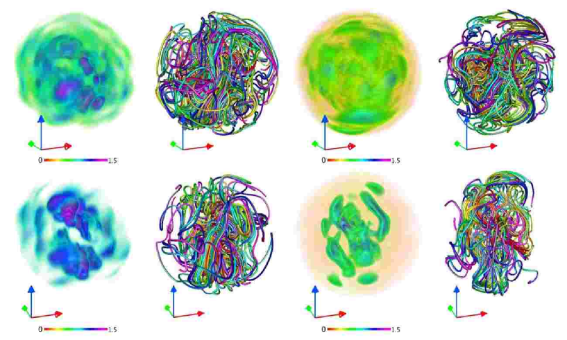
Figure 14: Above: kinetic energy density and velocity field lines at late times in Run D5 (left), and magnetic energy density and magnetic field files at the same time for the same run. Below: same quantities for Run D7. Note the development of anisotropies in the presence of large $\Omega$ in this run.

A second trend is indicated in Figure 12: namely the orientation of the dipole moment onto the axis of rotation seems less erratic with decreasing Rossby and Ekman numbers. That is, there are more eddy turnover times (in units of $R/U$) between the near reversals as $R_{O}$ and $E_{K}$ are decreased, and the projection of the dipole moment on the unit sphere gets more localized around the two “poles” defined by the axis of rotation. We borrow here the term “reversal” from the palaeomagnetic record, where during a reversal the orientation of the dipole moment changes about $180^{\circ}$ and its amplitude decreases, in opposition to an “excursion” in which the direction and the orientation of the dipole moment changes in a short period of time without resulting in a full reversal [33].

To verify this behavior, in Runs D6, D7, and D8 we successively decreased $R_{O}$ and $E_{K}$ while keeping the other parameters constant. At the present resolution, we could not decrease the values of $R_{O}$ and $E_{K}$ below the values for run D8 while keeping the boundary layer well resolved. In geodynamo simulations, a similar effect was reported, and it was noted that the behavior of the dipole moment was controlled by the amplitude of the Rossby number, independently of the values of the Ekman and Rayleigh numbers [26].

Figure 12 shows the trace of the dipole moment $\mu$ on the surface of the unit sphere, its amplitude, and the cosine of the angle between $\mu$ and $\Omega$ for runs D3, D5, and D7. While in Run D3 the trace of $\mu$ fills the entire surface of the sphere, as $R_{O}$ and $E_{K}$ are decreased $\mu$ seems to fluctuate around two regions in opposite sides of the sphere. These regions get more localized with decreasing $R_{O}$ and $E_{K}$. Also, the time between excursions of $\mu$ outside these regions gets larger, as shown by $\cos(\gamma)$. In Run D7, after a transient that finishes at $t\approx 80$, $\cos(\gamma)$ stays at $1$ or $-1$ for $\approx 20$ turnover times before changing sign rapidly. It is also worth noticing that as $R_{O}$ and $E_{K}$ decrease, the time it takes the system to develop a dipole moment of order one gets larger (see the evolution of $|\mbox{\boldmath$\mu$}|$ at early times in Figure 12). This is also observed in the time evolution of the magnetic energy (see Figure 13). Instead of having an exponential growth of $E_{M}$ at early times as in Runs D1 to D5, Runs D6 to D8 show a more intermittent behavior: magnetic energy grows in rapid “bursts” and stays around that value until a new burst increases the magnetic energy again. In Run D7, this process saturates around $t\approx 80$ and no further change in the average value of $E_{M}$ is observed. It is possible that the slow-down during the kinematic dynamo regime is a consequence of a quasi-two-dimensionalization of the flow by the high rotation rate; this remains to be investigated fully.

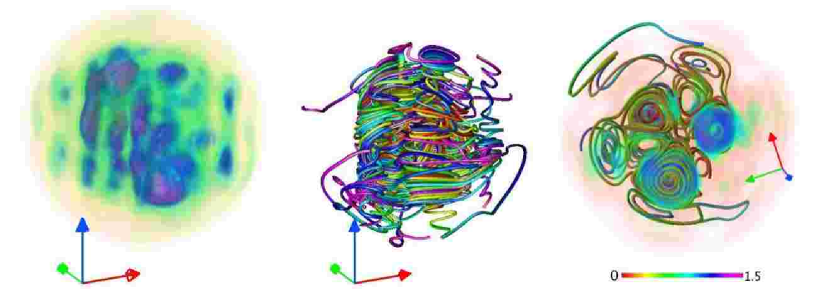
Figure 15: Kinetic energy density (left), velocity field lines (middle), and view from top of the kinetic energy density superposed with velocity field lines (right) in run D10, before magnetic energy is introduced. Note the columnar structures in the velocity field aligned along $\Omega$ (in the $z$ direction).

Figure 14 shows visualizations of energy densities and field lines at late times in Runs D5 and D7. The development of anisotropies in the velocity and magnetic fields can be observed in run D7, which has the highest rotation rate attained of $\Omega=16$. Indeed, as $\Omega$ is increased the velocity field shows a tendency to develop columns, with mechanical energy concentrated in cylindrical structures aligned along $\Omega$ and with a larger component of $v_{\phi}$ than of $v_{z}$. The velocity field in these column is helical, although in general the total mechanical helicity of the flow fluctuates in time around zero. These structures are observed before the magnetic field is introduced (although they persist as the magnetic energy grows) and seem to be the result of the Taylor-Proudman effect (see e.g. [34, 35]). It is a trend observed through runs D5 to D10 (see Figure 15 for an example).

Run D9 experiments with lowering the angle between the forcing’s axis of symmetry and the axis of rotation to $\alpha=20^{\circ}$, and the dipole becomes more difficult to excite (as evidenced by a smaller growth rate in the kinematic dynamo regime). Indeed, dynamo action could not be excited below $15^{\circ}$ for the values of Reynolds numbers explored, as the resulting driven flow approaches axisymmetry.

Figure 16: (a) Trace of the dipole moment on the surface of the unit sphere (above) and amplitude of the dipole moment as a function of time (below) for Run D11. (b) Same quantities for run D12.

Run D10 is actually part of a set of experiments (Runs D10 to D12; again, see Table 1) with forcing functions that are non-axisymmetric, and which may also inject mechanical helicity (Runs D11 and D12). Run D10, having no net mechanical helicity, shows no big differences in the evolution of global quantities from the previously discussed runs. The dipole develops but its orientation wanders randomly, with some preferred orientation perpendicular to $\Omega$. In this case, axisymmetry is broken by the forcing directly instead of by a non-zero angle between an axisymmetry forcing and the axis of rotation.

Runs D11 and D12 have non-axisymmetric forcing that injects mechanical helicity. The forcing for these runs is given by equation (20) with coefficients

$$\xi^{f}_{3,3,0}=5\xi^{f}_{-3,3,0}=F_{0},\;\;\xi^{f}_{3,3,0<m\leq 3}=5\xi^{f}_{-3,3,0<m\leq 3}=F_{0}(1+i),$$ (21)

with $F_{0}=1.7$. In the presence of net helicity, dynamo excitation suddenly becomes much easier (as evidenced by a much larger growth rate of magnetic energy during the kinematic regime), and the ultimate saturation occurs at $E_{M}/E_{V}\approx 2$: more magnetic than kinetic, with magnetic helicity, having sign opposite that of the mechanical helicity inversely cascading to the large scales. As a result, the system is dominated by a helical magnetic field at the largest available scale.

An interesting qualitative argument from mean field theory [36, 37] (which assumes large scale separations and often some form of periodic boundary conditions, as do all “$\alpha$-effect” calculations) can be seen to anticipate this result as follows. From mean field theory , the induction equation for the mean magnetic field $\overline{\bf B}$ (assuming there is no mean flow $\overline{\bf U}$) is

$$\frac{\partial\overline{\bf B}}{\partial t}=\alpha\nabla\times\overline{\bf B}+\beta\nabla^{2}\overline{\bf B}.$$ (22)

Here, $\alpha$ is proportional to minus the kinetic helicity of the flow [36, 38, 37], and $\beta$ is a turbulent magnetic diffusivity. Dotting equation (22) with the mean vector potential $\overline{\bf A}$ (such as $\overline{\bf B}=\nabla\times\overline{\bf A}$) and integrating over volume, an equation for the evolution of the mean magnetic helicity $\overline{H_{M}}$ is obtained,

$$\frac{d\overline{H_{M}}}{dt}=\alpha\overline{E_{M}}+\beta\nabla^{2}\overline{H_{J}},$$ (23)

where $\overline{E_{M}}$ is the mean magnetic energy and $\overline{H_{J}}$ is the mean current helicity. As a result, if magnetic diffusion is neglected, the dynamo process injects into the mean (large) scales magnetic helicity of opposite sign than the kinetic helicity, and in the small scales magnetic helicity of the same sign. This effect has been observed before in numerical dynamo simulations with periodic boundary conditions [28, 31]. The large scale magnetic helicity then inverse-cascades to the largest available scale in the system, while the small scale magnetic helicity is transferred to smaller scales where it is dissipated [39]. As a result, at late times the system is dominated by a large scale magnetic field with magnetic helicity of opposite sign to that of the kinetic helicity injected by the forcing.

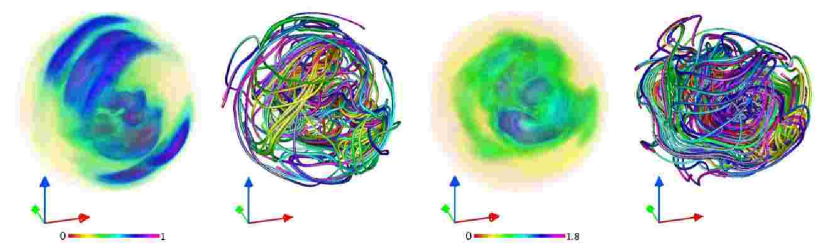
Figure 17: Kinetic energy density and velocity field lines (left), and magnetic energy density and magnetic field lines (right) at the same time in the saturated state of run D12. The axes are aligned as in Figure 16.

As seen in Figure 16, the dipolar orientation in D11 seems to have a preference for being perpendicular to $\Omega$. For run D12, whose forcing function differs in its orientation to $\Omega$ by $90^{\circ}$, the dipole orientation seems to remain in a single hemisphere (see Figure 16) and its tip precesses about $\Omega$. Figure 17 shows energy density and field lines in the saturated steady state of run D12. The axes are aligned as in Figure 16. As is often the case with helical flows, the geometry of the flow is more complex than in the non-helical runs. These runs in which a net sign of mechanical helicity is sustained by the mechanical forcing were continued for several thousands turnover times, and no reversals of the dipole moment were observed. The dipole moment seems to fluctuate around a preferred orientation with only short excursions of the dipole to the opposite hemisphere.

5 Discussion and future directions

By solving the mechanically-forced MHD equations inside a rotating conducting spherical boundary, we have found that a bewilderingly wide variety of dynamo behavior is possible for a magnetic Prandtl number of unity. The behavior is sensitive to mechanical and magnetic Reynolds numbers, to rotation rate, and more indirectly to the Ekman number. It is also sensitive to the geometry and strength of the forcing functions and their relation to the axis of rotation. We have only begun to explore this multidimensional parameter space. Note we have not made much effort to tailor the forcing functions we have chosen to model what the mechanical flows in planetary cores or stellar convective regions might be. Rather, we have been exploring dynamo behavior in the abstract, and feel somewhat overwhelmed by the variety of dynamo behavior that has been found. In this light, our attempt should be consider as an extension of dynamo simulations in periodic boundary conditions [27, 28, 31, 40, 29, 30] to consider the effect of boundaries and rotation, and not be compared with explorations of the space of parameters in realistic geodynamo simulations [10, 9, 13, 2, 26].

What has become clear is that the wholly spectral methods we are using, while accurate, do not scale well into the parameter regimes of planetary and astrophysical dynamos, which involve many orders of magnitude between the largest length scales in the flows and the Ekman or dissipation scales that also play a role in the process. This limitation afflicts all numerical attempts to explore planetary and stellar dynamos, particularly in view of the low magnetic Prandtl numbers that are expected to prevail there, in simulations [29, 30], and in liquid-sodium experiments [41, 42, 43, 44, 45]. But the rapid multiplication of the number of terms to compute in the convolution sums in equations (10) and (11) provides a rather intractable limitation on efforts to use our code without modification at higher Reynolds numbers than the few hundred we have explored here. What seems to be called for is an exploration of the possibilities of using fast transforms (for spherical harmonics [46, 47] and possibly for spherical Bessel functions [48, 49])to turn the code into a pseudospectral one in which the nonlinear terms are computed in configuration space rather than spectral space, as is commonly done for rectangular periodic boundary conditions [17] which would increase available resolution by many orders of magnitude. Our future investigations will explore this possibility.

We also intend to replace the conducting boundary by an insulating but mechanically-impenetrable one that will permit protrusion of the magnetic field into the vacuum region surrounding the shell (see e.g. [2]). It may be that forcing the magnetic field lines to return to the interior each time they get near the shell that is now playing a dynamical role in what we are seeing would be different in the case of an insulating shell. This raises some conceptual difficulties, since the problem of matching MHD fields on to vacuum electromagnetic ones has not been thoroughly solved. For example, one approximation that has been used has been to match magnetic fields at a spherical surface to magnetostatic ones outside, which involve a magnetic field that is derivable from a scalar potential and for which there is no electric field. However, Maxwell’s equations tell us that the tangential electric field must be continuous at any interface, and there is no reason why this tangential electric field should vanish or even be “small” immediately inside an insulating boundary of a conducting magnetofluid. The magnetostatic approximation may be the best we can do, but it would be desirable to have more justification for it than we presently have.

Finally, we need to devote attention to the geometry and strength of the forcing functions that are being employed and to study the effect of different forcing functions in dynamo action. Mechanical processes, convective and otherwise, are believed to power the dynamo in cases of geophysical or astrophysical interest. In the simulations discussed, we have no explanation, for example, why the “columns” or columnar vortices aligned along $\Omega$ form in the velocity field in runs toward the end of Table 1. It is clear the physical effect that is triggering their formation is the rotation alone, perhaps through a two-dimensionalization of the flow via the Taylor-Proudman effect [34, 35, 8]. This is a different process than the conventional explanation for the formation of columns in planetary interiors, which involves both thermal convection and rotation [50], since thermal convection is completely absent in our incompressible MHD formulation.

References

References

- [1] P. D. Mininni and D. C. Montgomery. Magnetohydrodynamic activity inside a sphere. Phys. Fluids, 18:116602, 2006.
- [2] M. Kono and P. H. Roberts. Recent geodynamo simulations and observations of the geomagnetic field. Rev. Geophys., 40:1–53, 2002.
- [3] S. Chandrasekhar and P. C. Kendall. On force-free magnetic fields. Astrophys. J., 126:457–460, 1957.
- [4] D. C. Montgomery, L. Turner, and G. Vahala. Three-dimensional magnetohydrodynamic turbulence in cylindrical geometry. Phys. Fluids, 21:757–764, 1978.
- [5] L. Turner. Statistical mechanics of a bounded, ideal magnetofluid. Ann. Phys. (NY), 149:58–161, 1983.
- [6] J. Cantarella, D. DeTurck, H. Gluck, and M. Teytel. The spectrum of the curl operator on spherically symmetric domains. Phys. Plasmas, 7:2766–2775, 2000.
- [7] H. P. Greenspan. The theory of rotating fluids. Cambridge Univ. Press., Cambridge, 1968.
- [8] D. J. Acheson. Elementary fluid dynamics. Clarendon Press, Oxford, 1990.
- [9] K. Zhang and G. Schubert. Magnetohydrodynamics in rapidly rotating spherical systems. Annu. Rev. Fluid Mech., 32:409–443, 2000.
- [10] G. A. Glatzmaier and P. H. Roberts. A three-dimensional self-consistent computer simulation of a geomagnetic field reversal. Nature, 377:203–209, 1995.
- [11] G. A. Glatzmaier and P. H. Roberts. Rotation and magnetism of earth’s inner core. Science, 274:1887–1891, 1996.
- [12] U. R. Christensen, J. Aubert, P. Cardin, E. Dormy, S. Gibbons, G. A. Glatzmaier, E. Grote, Y. Honkura, C. Jones, M. Kono, M. Matsushima, A. Sakuraba, F. Takahashi, A. Tilgner, J. Wicht, and K. Zhang. A numerical dynamo benchmark. Phys. of the Earth and Plan. Int., 128:25–34, 2001.
- [13] P. H. Roberts and G. A. Glatzmaier. The geodynamo, past, present and future. Geophys. Astrophys. Fluid Dyn., 94:47–84, 2001.
- [14] H. K. Moffatt. Magnetic field generation in electrically conducting fluids. Cambridge Univ. Press, Cambridge, 1978.
- [15] B. T. Kress and D. C. Montgomery. Pressure determinations for incompressible fluids and magnetofluids. J. Plasma Phys., 64:371–377, 2000.
- [16] G. Gallavotti. Foundations of fluid dynamics. Springer Verlag, Berlin, 2002. pp. 83–87 ff.
- [17] C. Canuto, Y. Hussaini, A. Quarteroni, and T. Zang. Spectral methods in fluid dynamics. Springer Verlag, New York, 1988.
- [18] E. Dormy, P. Cardin, and D. Jault. MHD flow in a slightly differentially rotating spherical shell, with conducting inner core, in a dipolar magnetic field. Phys. of the Earth and Plan. Int., 160:15–30, 1998.
- [19] J. Clyne and M. Rast. A prototype discovery environment for analyzing and visualizing terascale turbulent fluid flow simulations. In R. F. Erbacher, J. C. Roberts, M. T. Grohn, and K. Borner, editors, Visualization and data analysis 2005, pages 284–294, Bellingham, Wash., 2005. SPIE. http://www.vapor.ucar.edu.
- [20] W. H. Matthaeus and D. Montgomery. Selective decay hypothesis at high mechanical and magnetic reynolds numbers. Ann. N. Y. Acad. Sci., 357:203–222, 1980.
- [21] A. C. Ting, W. H. Matthaeus, and D. Montgomery. Turbulent relaxation processes in magnetohydrodynamics. Phys. Fluids, 29:3261–3274, 1986.
- [22] R. Kinney, J. C. McWilliams, and T. Tajima. Coherent structures and turbulent cascades in two-dimensional incompressible magnetohydrodynamic turbulence. Phys. Plasmas, 2:3623–3639, 1995.
- [23] R. Grappin, A. Pouquet, and J. Léorat. Dependence on correlation of MHD turbulence spectra. Astron. Astrophys., 126:51–56, 1983.
- [24] A. Pouquet, M. Meneguzzi, , and U. Frisch. The growth of correlations in MHD turbulence. Phys. Rev. A, 33:4266–4276, 1986.
- [25] S. Ghosh, W. H. Matthaeus, , and D. C. Montgomery. The evolution of cross helicity in driven/dissipative two-dimensional magnetohydrodynamics. Phys. Fluids, 31:2171–2184, 1988.
- [26] U. R. Christensen and J. Aubert. Scaling properties of convection-driven dynamos in rotating spherical shells. Geophys. J. Int., 166:97–114, 2006.
- [27] M. Meneguzzi, U. Frisch, and A. Pouquet. Helical and nonhelical turbulent dynamos. Phys. Rev. Lett., 47:1060–1064, 1981.
- [28] A. Brandenburg. The inverse cascade and nonlinear alpha-effect in simulations of isotropic helical hydromagnetic turbulence. Astrophys. J., 550:824–840, 2001.
- [29] Y. Ponty, P. D. Mininni, D. C. Montgomery, J.-F. Pinton, H. Politano, and A. Pouquet. Numerical study of dynamo action at low magnetic prandtl numbers. Phys. Rev. Lett., 94:164502, 2005.
- [30] P. D. Mininni and D. C. Montgomery. Low magnetic prandtl number dynamos with helical forcing. Phys. Rev. E, 72:056320, 2005.
- [31] D. O. Gómez and P. D. Mininni. Direct numerical simulations of helical dynamo action: MHD and beyond. Nonlin. Proc. Geophys., 11:619–629, Dic 2004.
- [32] P. D. Mininni, D. O. Gómez, and S. M. Mahajan. Direct simulations of helical Hall-MHD turbulence and dynamo action. ApJ, 619:1019–1027, 2005.
- [33] J.-P. Valet, L. Meynadier, and Y. Guyodo. Geomagnetic dipole strength and reversal rate over the past two million years. Nature, 435:802–805, 2005.
- [34] G. I. Taylor. Experiments on the motion of solid bodies in rotating fluids. Proc. Roy. Soc. A, 104:213–218, 1923.
- [35] P. A. Davies. Experiments on taylor columns in rotating stratified flows. J. Fluid Mech., 54:691–717, 1972.
- [36] M. Steenbeck, F. Krause, and K.-H. Rädler. Berechnung der mittleren Lorentz-Feldstaerke fuer ein elektrisch leitendendes Medium in turbulenter, durch Coriolis-Kraefte beeinflußter Bewegung. Z. Naturforsch., 21a:369–376, 1966.
- [37] F. Krause and K.-H. Raedler. Mean-field magnetohydrodynamics and dynamo theory. Pergamon Press, New York, 1980.
- [38] A. Pouquet, U. Frisch, and J. Léorat. Strong MHD helical turbulence and the nonlinear dynamo effect. J. Fluid Mech., 77:321–354, 1976.
- [39] A. Alexakis, P. D. Mininni, and A. Pouquet. On the inverse cascade of magnetic helicity. Astrophys. J., 640:335–343, 2006.
- [40] A. Brandenburg and K. Subramanian. Astrophysical magnetic fields and nonlinear dynamo theory. Phys. Rep., 417:1–209, 2005.
- [41] A. Gailitis, O. Lielausis, E. Platacis, S. Dement’ev, A. Cifersons, G. Gerbeth, T. Gundrum, F. Stefani, M. Christen, and G. Will. Magnetic field saturation in the riga dynamo experiment. Phys. Rev. Lett., 86:003024, 2001.
- [42] R. Steiglitz and U. Müller. Experimental demonstration of a homogeneous two-scale dynamo. Phys. Fluids, 13:561–564, 2001.
- [43] F. Pétrélis, M. Bourgoin, L. Marié, J. Burguete, A. Chiffaudel, F. Daviaud, S. Fauve, P. Odier, and J.-F. Pinton. Nonlinear magnetic induction by helical motion in a liquid sodium turbulent flow. Phys. Rev. Lett., 90:174501, 2003.
- [44] D. R. Sisan, W. L. Shew, and D. P. Lathrop. Lorentz force effects in magneto-turbulence. Phys. Earth Plan. Int., 135:137–159, 2003.
- [45] E. J. Spence, M. D. Nornberg, C. M. Jacobson, R. D. Kendrick, and C. B. Forest. Observation of a turbulence-induced large scale magnetic field. Phys. Rev. Lett., 96:055002, 2006.
- [46] J. R. Driscoll and D. M. Healy Jr. Computing Fourier transforms and convolutions on the 2-sphere. Adv. Applied Math., 15:202–250, 1994.
- [47] M. Mohlenkamp. A fast transform for spherical harmonics. J. of Fourier Analysis and Appl., 5:159–184, 1999.
- [48] O. A. Sharafeddin, H. F. Bowen, D. J. Kouri, and D. K. Hoffman. Numerical evaluation of spherical Bessel transforms via fast Fourier transforms. J. Comp. Phys., 100:294–296, 1992.
- [49] M. J. Cree and P. J. Bones. Algorithms to numerically evaluate the Hankel transform. Computers Math. Applic., 26:1–12, 1993.
- [50] F. H. Busse. Thermal instabilities in rapidly rotating systems. J. Fluid Mech., 44:441–460, 1970.