Hilbert Space Becomes Ultrametric in the High Dimensional Limit: Application to Very High Frequency Data Analysis

Abstract

An ultrametric topology formalizes the notion of hierarchical structure. An ultrametric embedding, referred to here as ultrametricity, is implied by a natural hierarchical embedding. Such hierarchical structure can be global in the data set, or local. By quantifying extent or degree of ultrametricity in a data set, we show that ultrametricity becomes pervasive as dimensionality and/or spatial sparsity increases. This leads us to assert that very high dimensional data are of simple structure. We exemplify this finding through a range of simulated data cases. We discuss also application to very high frequency time series segmentation and modeling.

PACS: 02.50.-r, 05.45.Tp, 89.65.Gh, 89.20.-a

1 Introduction

The topology or inherent shape and form of an object is important. In data analysis, the inherent form and structure of data clouds are important. Quite a few models of data form and structure are used in data analysis. One of them is a hierarchically embedded set of clusters, – a hierarchy. It is traditional (since at least the 1960s) to impose such a form on data, and if useful to assess the goodness of fit. Rather than fitting a hierarchical structure to data (e.g., [23]), our recent work has taken a different orientation: we seek to find (partial or global) inherent hierarchical structure in data. As we will describe in this article, there are interesting findings that result from this, and some very interesting perspectives are opened up for data analysis and, potentially, perspectives also on the physics (or causal or generative mechanisms) underlying the data.

A formal definition of hierarchical structure is provided by ultrametric topology (in turn, related closely to p-adic number theory). We will return to this in section 2 below. First, though, we will summarize some of our findings.

Ultrametricity is a pervasive property of observational data. It arises as a limit case when data dimensionality or sparsity grows. More strictly such a limit case is a regular lattice structure and ultrametricity is one possible representation for it. Notwithstanding alternative representations, ultrametricity offers computational efficiency (related to tree depth/height being logarithmic in number of terminal nodes), linkage with dynamical or related functional properties (phylogenetic interpretation), and processing tools based on well known p-adic or ultrametric theory (examples: deriving a partition, or applying an ultrametric wavelet transform). In [11] and other works, Khrennikov has pointed to the importance of ultrametric topological analysis.

Local ultrametricity is also of importance. This can be used for forensic data exploration (fingerprinting data sets): see [15] and [16]; and to expedite search and discovery in information spaces: see [6] as discussed by us in [14], [18], and [19].

In section 2 we show how extent of ultrametricity is measured. Section 3 presents our main results on the remarkable properties of very high dimensional, or very sparse, spaces. As dimensionality or sparsity grow, so does the inherent hierarchical nature of the data in the space. In section 4.2 we then discuss application to very high frequency time series modeling.

2 Quantifying Degree of Ultrametricity

Summarizing a full description in Murtagh [14] we explored two measures quantifying how ultrametric a data set is, – Lerman’s and a new approach based on triangle invariance (respectively, the second and third approaches described in this section).

The triangular inequality holds for a metric space: $d(x,z)\leq d(x,y)+d(y,z)$ for any triplet of points $x,y,z$. In addition the properties of symmetry and positive definiteness are respected. The “strong triangular inequality” or ultrametric inequality is: $d(x,z)\leq\mbox{ max }\{d(x,y),d(y,z)\}$ for any triplet $x,y,z$. An ultrametric space implies respect for a range of stringent properties. For example, the triangle formed by any triplet is necessarily isosceles, with the two large sides equal; or is equilateral.

• Firstly, Rammal et al. [22] used discrepancy between each pairwise distance and the corresponding subdominant ultrametric. Now, the subdominant ultrametric is also known as the ultrametric distance resulting from the single linkage agglomerative hierarchical clustering method. Closely related graph structures include the minimal spanning tree, and graph (connected) components. While the subdominant provides a good fit to the given distance (or indeed dissimilarity), it suffers from the “friends of friends” or chaining effect.

• Secondly, Lerman [12] developed a measure of ultrametricity, termed H-classifiability, using ranks of all pairwise given distances (or dissimilarities). The isosceles (with small base) or equilateral requirements of the ultrametric inequality impose constraints on the ranks. The interval between median and maximum rank of every set of triplets must be empty for ultrametricity. We have used extensively Lerman’s measure of degree of ultrametricity in a data set. Taking ranks provides scale invariance. But the limitation of Lerman’s approach, we find, is that it is not reasonable to study ranks of real-valued (values in non-negative reals) distances defined on a large set of points.

• Thirdly, our own measure of extent of ultrametricity [14] can be described algorithmically. We examine triplets of points (exhaustively if possible, or otherwise through sampling), and determine the three angles formed by the associated triangle. We select the smallest angle formed by the triplet points. Then we check if the other two remaining angles are approximately equal. If they are equal then our triangle is isosceles with small base, or equilateral (when all triangles are equal). The approximation to equality is given by 2 degrees (0.0349 radians). Our motivation for the approximate (“fuzzy”) equality is that it makes our approach robust and independent of measurement precision.

A supposition for use of our measure of ultrametricity is that we can can define angles (and hence triangle properties). This in turn presupposes a scalar product. Thus we presuppose a complete normed vector space with a scalar product – a Hilbert space – to provide our needed environment.

Quite a general way to embed data, to be analyzed, in a Euclidean space, is to use correspondence analysis [17]. This explains our interest in using correspondence analysis: it provides a convenient and versatile way to take input data in many varied formats (e.g., ranks or scores, presence/absence, frequency of occurrence, and many other forms of data) and map them into a Euclidean, factor space.

3 Ultrametricity and Dimensionality

3.1 Distance Properties in Very Sparse Spaces

Murtagh [14], and earlier work by Rammal et al. [21, 22], has demonstrated the pervasiveness of ultrametricity, by focusing on the fact that sparse high-dimensional data tend to be ultrametric. In such work it is shown how numbers of points in our clouds of data points are irrelevant; but what counts is the ambient spatial dimensionality. Among cases looked at are statistically uniformly (hence “unclustered”, or without structure in a certain sense) distributed points, and statistically uniformly distributed hypercube vertices (so the latter are random 0/1 valued vectors). Using our ultrametricity measure, there is a clear tendency to ultrametricity as the spatial dimensionality (hence spatial sparseness) increases.

As [9] also show, Gaussian data behave in the same way and a demonstration of this is seen in Table 1. To provide an idea of consensus of these results, the 200,000-dimensional Gaussian was repeated and yielded on successive runs values of the ultrametricity measure of: 0.96, 0.98, 0.96.

No. points	Dimen.	Isosc.	Equil.	UM
Uniform
100	20	0.10	0.03	0.13
100	200	0.16	0.20	0.36
100	2000	0.01	0.83	0.84
100	20000	0	0.94	0.94
100	200000	0	0.97	0.97
Hypercube
100	20	0.14	0.02	0.16
100	200	0.16	0.21	0.36
100	2000	0.01	0.86	0.87
100	20000	0	0.96	0.96
100	200000	0	0.97	0.97
Gaussian
100	20	0.12	0.01	0.13
100	200	0.23	0.14	0.36
100	2000	0.04	0.77	0.80
100	20000	0	0.98	0.98
100	200000	0	0.96	0.96

Table 1: Typical results, based on 300 sampled triangles from triplets of points. For uniform, the data are generated on [0, 1]; hypercube vertices are in $\{0,1\}^{\mbox{Dimen}}$, and for Gaussian, the data are of mean 0, and variance 1. Dimen. is the ambient dimensionality. Isosc. is the number of isosceles triangles with small base, as a proportion of all triangles sampled. Equil. is the number of equilateral triangles as a proportion of triangles sampled. UM is the proportion of ultrametricity-respecting triangles (= 1 for all ultrametric).

In the following, we explain why high dimensional and/or sparsely populated spaces are ultrametric.

As dimensionality grows, so too do distances (or indeed dissimilarities, if they do not satisfy the triangular inequality). The least change possible for dissimilarities to become distances has been formulated in terms of the smallest additive constant needed, to be added to all dissimilarities [24, 4, 5, 20]. Adding a sufficiently large constant to all dissimilarities transforms them into a set of distances. Through addition of a larger constant, it follows that distances become approximately equal, thus verifying a trivial case of the ultrametric or “strong triangular” inequality. Adding to dissimilarities or distances may be a direct consequence of increased dimensionality.

For a close fit or good approximation, the situation is not as simple for taking dissimilarities, or distances, into ultrametric distances. A best fit solution is given by [7] (and software is available in R [10]). If we want a close fit to the given dissimilarities then a good choice would avail either of the maximal inferior, or subdominant, ultrametric; or the minimal superior ultrametric. Stepwise algorithms for these are commonly known as, respectively, single linkage hierarchical clustering; and complete link hierarchical clustering. (See [3, 12, 13] and other texts on hierarchical clustering.)

3.2 No “Curse of Dimensionality” in Very High Dimensions

Bellman’s [2] “curse of dimensionality” relates to exponential growth of hypervolume as a function of dimensionality. Problems become tougher as dimensionality increases. In particular problems related to proximity search in high-dimensional spaces tend to become intractable.

In a way, a “trivial limit” (Treves [25]) case is reached as dimensionality increases. This makes high dimensional proximity search very different, and given an appropriate data structure – such as a binary hierarchical clustering tree – we can find nearest neighbors in worst case $O(1)$ or constant computational time [14]. The proof is simple: the tree data structure affords a constant number of edge traversals.

The fact that limit properties are “trivial” makes them no less interesting to study. Let us refer to such “trivial” properties as (structural or geometrical) regularity properties (e.g. all points lie on a regular lattice).

First of all, the symmetries of regular structures in our data may be of importance. For example, processing of such data can exploit these regularities.

Secondly, “islands” or clusters in our data, where each “island” is of regular structure, may be of interpretational value.

Fourthly, and finally, regularity of particular properties does not imply regularity of all properties. So, for example, we may have only partial existence of pairwise linkages.

Thus we see that in very high dimensions, and/or in very (spatially) sparse data clouds, there is a simplification of structure, which can be used to mitigate any “curse of dimensionality”. Figure 1 shows how the distances within and between clusters become tighter with increase in dimensionality.

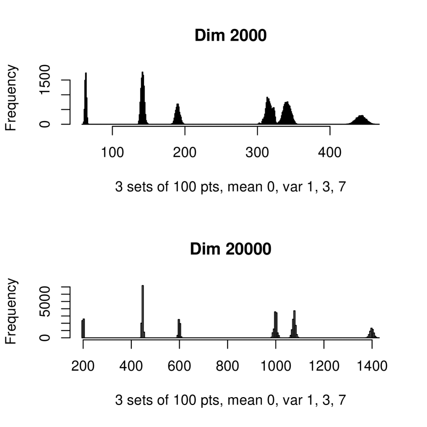
Figure 1: An illustration of how “symmetry” or “structure” can become increasingly pronounced as dimensionality increases. Shown are two simulations, each with 3 sub-populations of Gaussian-distributed data, in, respectively, ambient dimensions of 2000 and 20,000. These simulations correspond to the 3rd last, and 2nd last, rows of Table 1.

3.3 Gaussian Clusters in Very High Dimensions

3.3.1 Introduction

We will distinguish between cluster characteristics as follows:

1. cluster size: number of points per cluster;

2. cluster location: here, mean, identical on every dimension;

3. cluster scale: here, standard deviation, identical on every dimension.

These cluster characteristics are simple ones, and future work will consider greater sophistication.

In the homogeneous clouds studied in Table 1 it is seen that the isosceles (with small base) case disappeared early on, as dimensionality increased greatly, to the advantage of the equilateral case of ultrametricity. So the points become increasingly equilateral-related as dimensionality grows. This is not the case when the data in clustered, as we will now see.

3.3.2 Clusters with Different Locations, Same Scale

Table 2 is based on two clusters, and shows how isosceles triangles increasingly dominate as dimensionality grows. Figure 2 illustrates low and high dimensionality scenarios relating to Table 2. There is clear confirmation in this table as to how interrelationships in the cluster become more compact and, in a certain sense, more trivial, in high dimensions. This does not obscure the fact that we indeed have hierarchial relationships becoming ever more pronounced as dimensionality, and hence relative sparsity, increase. These observations help us to see quite clearly just how hierachical relationships come about, as ambient dimensionality grows.

No. points	Dimen.	Isosc.	Equil.	UM
200	20	0.08	0	0.08
200	200	0.19	0.04	0.23
200	2000	0.42	0.20	0.62
200	20000	0.74	0.22	0.96
200	20000	0.7	0.28	0.98
200	20000	0.77	0.21	0.98
200	20000	0.76	0.21	0.98
200	20000	0.75	0.24	0.99
200	20000	0.73	0.25	0.98

Table 2: Results based on 300 sampled triangles from triplets of points. Two Gaussian clusters, each of 100 points, were used in each case. One point set was of mean 0, and the other of mean 10, on each dimension. The standard deviations on each dimension were 1 in all cases. Column headings are as in Table 1. Five further results are given for the 20,000-dimension case to show variability.

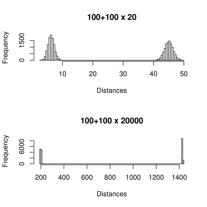
Figure 2: A further illustration of how “symmetry” or “structure” can become increasingly pronounced as dimensionality increases, relating to the $200\times 20$ and $200\times 20,000$ (first of the succession of rows) cases of Table 2. These are histograms of all interpoint distances, based on two Gaussian clusters. The first has mean 0 and standard deviation 1 on all dimensions. The second has mean 10 and standard deviation 1 on all dimensions.

3.3.3 Clusters with Different Locations, Different Scales

A more demanding case study is now tried. We generate 50 points per cluster with the following characteristics: mean 0, standard deviation 1, on each dimension; mean 3, standard deviation 2, on each dimension; mean 5, standard deviation 1, on each dimension; and mean 8, standard deviation 3, on each dimension. Table 3 shows the results obtained. Here we have not achieved quite the same level of ultrametricty, due to slower growth in ultrametricity which is, in turn, due to the more murky, less dermarcated, but undoubtdely clustered, set of data. Figure 3 illustrates this: this histogram shows one dimension, where we note that means of the Gaussians are at 0, 3, 5 and 8.

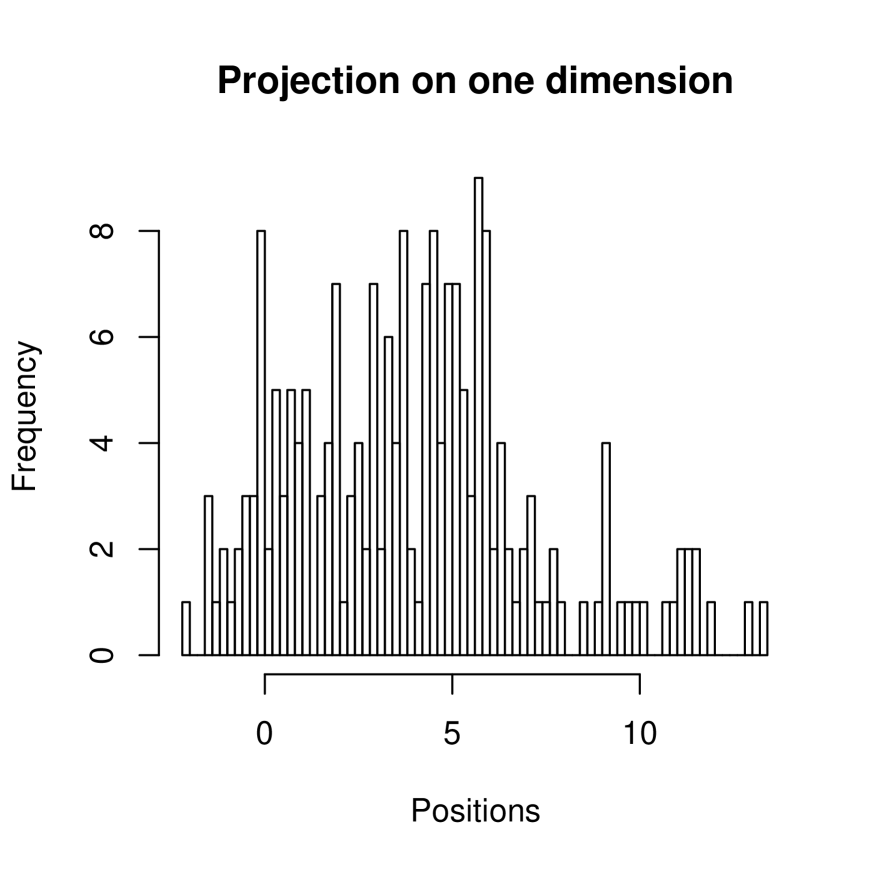
Figure 3: A projection onto one dimension, to illustrate the less than clearcut clustering problem addressed. There are four Gaussians here, each of 50 realizations, with means at 0, 3, 5 and 8, and with respective standard deviations of 1, 2, 1, 3.

No. points	Dimen.	Isosc.	Equil.	UM
200	20	0.04	0.01	0.05
200	200	0.11	0.05	0.16
200	2000	0.28	0.06	0.34
200	20000	0.5	0.08	0.58
200	200000	0.55	0.11	0.66

Table 3: Results based on 300 sampled triangles from triplets of points. Four Gaussian clusters, each of 50 points, were used in each case. See text for details of properties of these clusters.

When we look closer at Table 3, as shown in Figure 4, the compaction of distances is again very interesting. We verified the 7 peaks found in the lower histogram in Figure 4, and available but confusedly overlapping and ill-defined in the upper histogram of Figure 4.

What we find for the 7 peaks is as follows. Distances within the clusters correspond to: peaks 1, 2, 3 and (again) 1. That two clusters are associated with one peak is clear from the fact that two of our clusters are of identical scale.

We can examine inter-cluster distances and we found these to be associated with peaks: 2, 3, 4, 5, 6, 7. Given 4 clusters, we could well have up to 6 possible additional peaks.

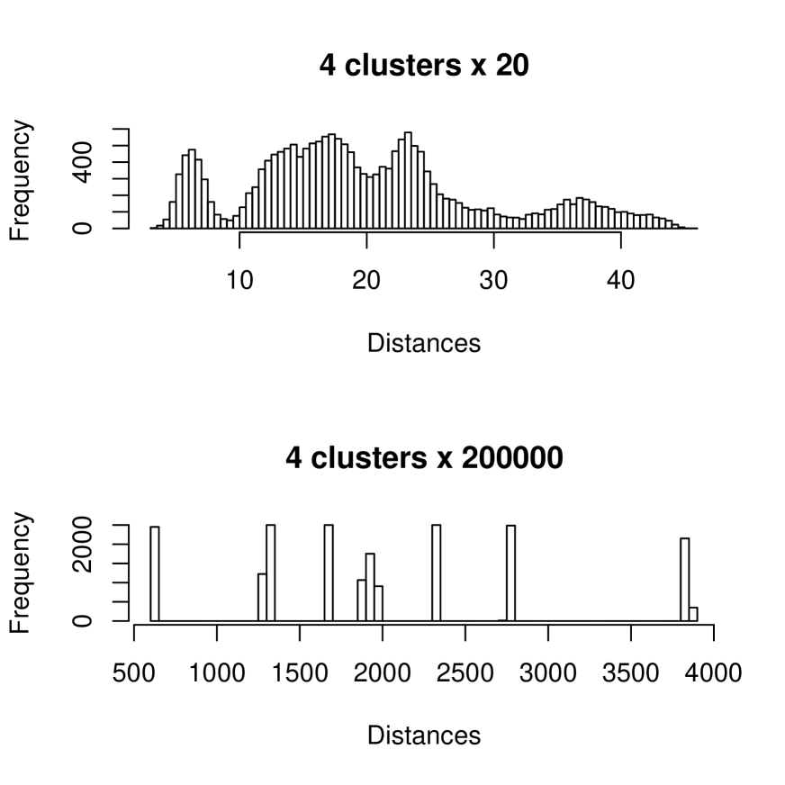
Figure 4: Compaction of distances with rise in dimensionality: 4 clusters, substantially overlapping are the basis for the histograms of all pairwise distances. Top: ambient dimensionality 20. Bottom: ambient dimensionality 200,000.

3.3.4 Conclusions on High Dimensional Gaussian Clouds

From these case studies, it is clear that increased dimensionality sharpens and distinguishes the clusters. If we can embed data – any data – in a far higher ambient dimensionality, without destroying the interpretable relationships in the data, then we can so much more easily read off the clusters.

To read off clusters, including memberships and properties, our findings can be summarized as follows.

For cluster size (i.e., numbers of points per cluster), sampling alone can be used, and we do not pursue this here.

For cluster scale (i.e., standard deviation, assumed the same on each dimension), we associate each cluster, or a pair of clusters, with each peak. The total number of peaks gives an upper bound on the number of clusters. (For $k$ clusters, we have $\leq k+k\cdot(k-1)/2$ peaks.)

Using cluster scale also permits use of the following cluster model: suppose that all clusters are defined to have intra-cluster distance that is less than inter-cluster distance. Then it follows that the peaks of lower distance correspond to the clusters (as opposed to pairs of clusters).

An example of this is as follows. In Figure 4, lower panel, we read from left to right, applying the following algorithm: select the first $k$ peaks as clusters, and ask: are there sufficient peaks to represent all inter-cluster pairs? If we choose $k=3$, there remain 4 peaks, which is too many to account for the inter-cluster pairs (i.e., $3\cdot(3-1)/2)$). So we see that Figure 4 is incompatible with $k=3$ or the presence of just 3 clusters.

Consequently we move to $k=4$, and see that Figure 4 is consistent with this.

A further identifiability assumption is reasonable albeit not required: that all smallest peaks be associated with intra-cluster distances. This need not be so, since we could well have a dense cluster superimposed on a less dense one. However it is a reasonable parimony assumption. Supported by this assumption, Figure 4 points to a minimum of 4 clusters in the data, with up to 4 peaks (read off from left to right, i.e., in increasing order of distance) corresponding to these clusters.

4 Applications

4.1 Data Recoding in the Correspondence Analysis Tradition

The iris data has been very widely used as a toy data set since Fisher used it in 1936 ([8], taken from [1]) to exemplify discriminant analysis. It consists of 150 iris flowers, each characterized by 4 petal and sepal, width and breadth, measurements. On the one hand, therefore, we have the 150 irises in $\mathbb{R}^{4}$. Next, each variable value was recoded by us to be a rank (all ranks of a given variable considered) and the rank was boolean-coded (viz., for the top rank variable value, $1000\dots$, for the second rank variable value, $0100\dots$, etc.). Following removal of zero total columns, the second data set defined the 150 irises in $\mathbb{R}^{123}$. Actually, this definition of the 150 irises is in fact in $\{0,1\}^{123}$.

Our triangle-based measure of the degree of ultrametricity in a data set (here the set of irises), with 0 = no ultrametricity, and 1 = every triangle an ultrametric-respecting one, gave the following: for irises in $\mathbb{R}^{4}$, 0.017; and for irises in $\{0,1\}^{123}$: 0.948.

This provides a nice illustration of how recoding can dramatically change the picture provided by one’s data. In chapter 3 of [17] it is discussed just what change in the data cloud is caused by the recoding. Our objective here is not to pursue the goodness of fit or otherwise of one data encoding vis-à-vis another. Instead our objective is to point out how data encoding influences directly (and at times remarkably) the data cloud’s ultrametricity, or ease of being hierarchically embedded.

In correspondence analysis, the $\chi^{2}$ distance when used on data tables with constant marginal sums becomes a weighted Euclidean distance. This is important for us as data analyst, because it means that we can directly influence the analysis by equi-weighting, say, the table rows in the following way: we double the row vector values by including an absence (0 value) whenever there is a presence (1 value) and vice versa. Or for a table of percentages, we take both the original value $x$ and $100-x$. In the correspondence analysis tradition [3, 17] this is known as doubling (dédoublement). More generally, booleanizing, or making qualitative, data in this way, for a varying (value-dependent) number of target value categories (or modalities) leads to the form of coding known as complete disjunctive form.

Such coding increases the embedding dimension, and data sparseness. From our example of recoding the Fisher data, such coding can influence degree of ultrametricity. We conclude that careful data coding can increase the extent to which our data is inherently hierarchical. Furthermore the latter in turn may be beneficial in enhancing data interpretability (for example, by unravelling phylogenetic aspects expressed by the data).

4.2 Application to High Frequence Data Analysis

In this section we establish proof of concept for application of the foregoing work to analysis of very high frequency univariate time series signals.

Consider each of the cases considered in section 3.3, expressed there as $n\times m$ arrays, as instead representing $n$ segments, each of (contiguous) length $m$, of a time series or one-dimensional signal. Assuming our aim is to cluster these segments on the basis of their properties, then it is reasonable to require that they be non-overlapping. The $n$ segments could come from anywhere, in any order, in the time series. So for the case of an $n\times m$ array considered previously, then implies a time series of length at least $nm$. The most immediate way to construct the time series is to raster scan the $n\times m$ array, although alternatives come readily to mind.

The methodology discussed in section 3.3 then is seen to be also a time series segmentation approach, facilitating the characterizing of the segments used.

To explore this further we consider a time series consisting of two ARIMA (autoregressive integrated moving average) models, with parameters: order, autoregression coefficients, moving average coefficients, and a “mildly longtailed” set of innovations based on the Student t distribution with 5 degrees of freedom. Figures 5 and 6 show samples of these time series segments. Figures 7 and 8 show histograms of these samples.

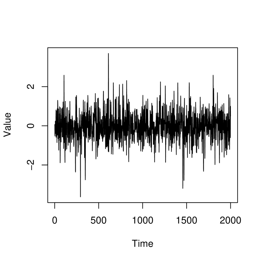
Figure 5: Sample (using first 1000 values) of a time series segment, based on the first ARIMA set of parameters. (Order 2 AR parameters: $0.8897,-0.4858$, MA parameters: $-0.2279,0.2488$.)

Figure 6: Sample (using first 1000 values) of a time series segment, based on the second ARIMA set of parameters. (Order 2 AR parameters: $0.2897,-0.1858$, MA parameters: $-0.7279,0.7488$.)

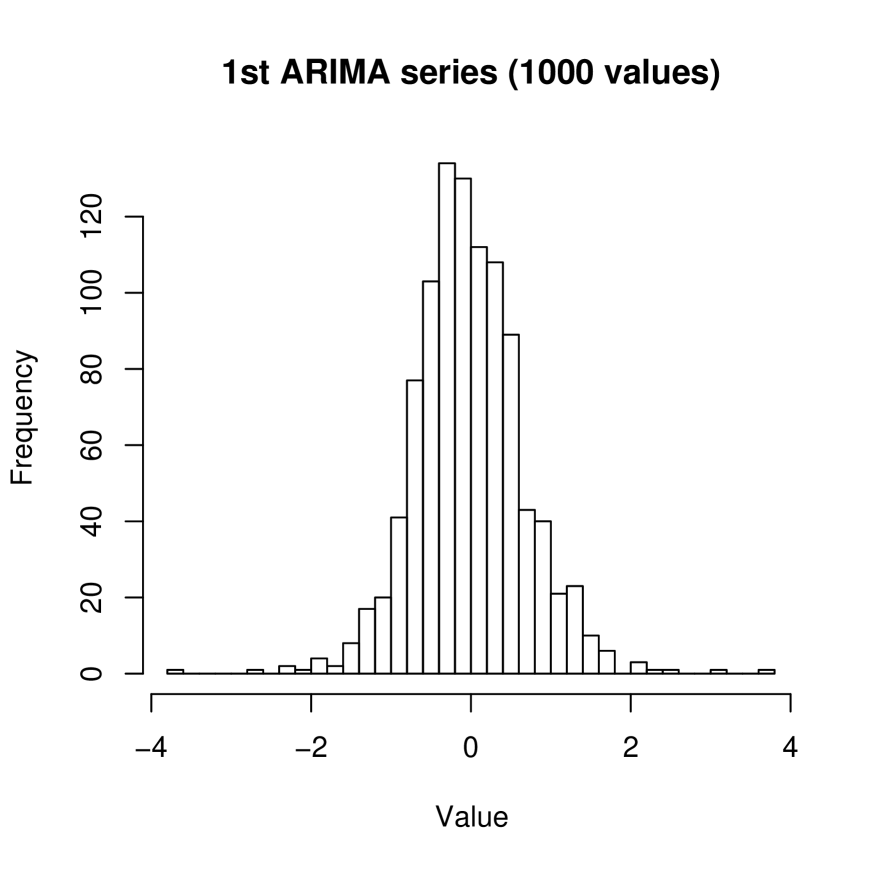
Figure 7: Histogram of sample (using first 1000 values) of time series segment shown in Figure 5.

Figure 8: Histogram of sample (using first 1000 values) of time series segment shown in Figure 6.

Table 4 shows typical results obtained in regard to ultrametricity. The dimensionality can be considered as the embedding dimension. Here, although ultrametricity increases, and the equilateral configuration seems to be increasing but with decrease of the isosceles with small base configuration, we do not consider it of practical relevance to test with even higher ambient dimensionalities. It is clear from the data, especially Figures 7 and 8, that the two signal models are very close in their properties.

Examining the histograms of all inter-pair time series segments, both intra and inter cluster, we find the clearly distinguished peaks shown in Figure 9. As before, we use Euclidean distance between time series segments or vectors. (We note that normalization or other transformation is not particularly relevant here. In fact we want to distinguish between inter and intra cluster cases. Furthermore the unweighted Euclidean distance is consistent with our use of angles to quantify triangle invariants, and hence respect for ultrametricity properties.)

No. time series	Dimen.	Isosc.	Equil.	UM
100	2000	0.17	0.32	0.49
100	20000	0.15	0.5	0.65
100	200000	0.03	0.57	0.60

Table 4: Results based on 300 sampled triangles from triplets of points. Two sets of the ARIMA models are used, each of 50 realizations.

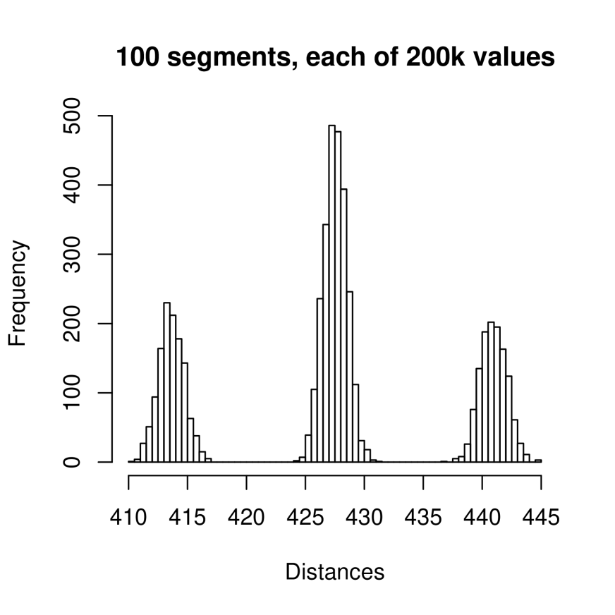
Figure 9: Histogram of distances from 100 time series segments, using 50 segments each from the two ARIMA models, and using an embedding dimensionality of 200,000.

We find clearly distinguishable peaks in Figure 9. The lower and the higher peaks belong to the two ARIMA components. The central peak belongs to the inter-cluster distances.

We have shown that our methodology can be of use for time series segmentation and for model identifiability. We will assess this further in future work. Given the use of a Hilbert space as the essential springboard of all aspects of this work, it would appear that generalization of this work to multivariate time series analysis is straightforward. What remains important, however, is the availability of very large embedding dimensionalities, i.e. very high frequency data streams.

5 Conclusions

What we have observed in all of this work is that in the limit of high dimensionality a Hilbert space becomes ultrametric.

It has been our aim in this work to link observed data with an ultrametric topology for such data. The traditional approach in data analysis, of course, is to impose structure on the data. This is done, for example, by using some agglomerative hierarchical clustering algorithm. We can always do this (modulo distance or other ties in the data). Then we can assess the degree of fit of such a (tree or other) structure to our data. For our purposes, here, this is unsatisfactory.

• Firstly, our aim was to show that ultrametricity can be naturally present in our data, globally or locally. We did not want any “measuring tool” such as an agglomerative hierarchical clustering algorithm to overly influence this finding. (Unfortunately [22] suffers from precisely this unhelpful influence of the “measuring tool” of the subdominant ultrametric. In other respects, [22] is a seminal paper.)

• Secondly, let us assume that we did use hierarchical clustering, and then based our discussion around the goodness of fit. This again is a traditional approach used in data analysis, and in statistical data modeling. But such a discussion would have been unnecessary and futile. For, after all, if we have ultrametric properties in our data then many of the widely used hierarchical clustering algorithms will give precisely the same outcome, and furthermore the fit is by definition optimal.

We have described an application of this work to very high frequency signal processing. The twin objectives are signal segmentation, and model identification. We have noted that a considerable amount of this work is model-based: we require assumptions (on clusters, and on model(s)) for identifiability.

Motivation for this work includes the availability of very high frequency data streams in various fields (physics, engineering, finance, meteorology, bio-engineering, and bio-medicine). By using a very large embedding dimensionality, we are approaching the data analysis on a very gross scale, and hence furnishing a particular type of multiresolution analysis. That this is worthwhile has been shown in our case studies.

References

- [1] E. Anderson, The irises of the Gape peninsula, Bull. Amer. Iris Soc., 59, 2–5, 1935.
- [2] R. Bellman, Adaptive Control Processes: A Guided Tour, Princeton University Press, 1961.
- [3] J.P. Benzécri, L’Analyse des Données, Tome I Taxinomie, Tome II Correspondances, 2nd ed., Dunod, Paris, 1979.
- [4] F. Cailliez and J.P. Pagès, Introduction à l’Analyse de Données, SMASH (Société de Mathématiques Appliquées et de Sciences Humaines), Paris, 1976.
- [5] F. Cailliez, The analytical solution of the additive constant problem, Psychometrika, 48, 305–308, 1983.
- [6] E. Chávez, G. Navarro, R. Baeza-Yates and J.L. Marroquín, Proximity searching in metric spaces, ACM Computing Surveys, 33, 273–321, 2001.
- [7] G. de Soete, A least squares algorithm for fitting an ultrametric tree to a dissimilarity matrix, Pattern Recognition Letters, 2, 133–137, 1986.
- [8] R.A. Fisher, The use of multiple measurements in taxonomic problems, The Annals of Eugenics, 7, 179–188, 1936.
- [9] P. Hall, J.S. Marron and A. Neeman, Geometric representation of high dimension low sample size data, Journal of the Royal Statistical Society B, 67, 427–444, 2005.
- [10] K. Hornik, A CLUE for CLUster Ensembles, Journal of Statistical Software, 14 (12), 2005.
- [11] A. Khrennikov, Non-Archimedean Analysis: Quantum Paradoxes, Dynamical Systems and Biological Models, Kluwer, 1997.
- [12] I.C. Lerman, Classification et Analyse Ordinale des Données, Paris, Dunod, 1981.
- [13] F. Murtagh, Multidimensional Clustering Algorithms, Physica-Verlag, 1985.
- [14] F. Murtagh, On ultrametricity, data coding, and computation, Journal of Classification, 21, 167–184, 2004.
- [15] F. Murtagh, Identifying the ultrametricity of time series, European Physical Journal B, 43, 573–579, 2005.
- [16] F. Murtagh, A note on local ultrametricity in text, http://arxiv.org/pdf/cs.CL/0701181, 2007.
- [17] F. Murtagh, Correspondence Analysis and Data Coding with R and Java, Chapman & Hall/CRC, 2005.
- [18] F. Murtagh, From data to the physics using ultrametrics: new results in high dimensional data analysis, in A.Yu. Khrennikov, Z. Rakić and I.V. Volovich, Eds., p-Adic Mathematical Physics, American Institute of Physics Conf. Proc. Vol. 826, 151–161, 2006.
- [19] F. Murtagh, G. Downs and P. Contreras, Hierarchical clustering of massive, high dimensional data sets by exploiting ultrametric embedding, 2007, submitted.
- [20] E. Neuwirth and L. Reisinger, Dissimilarity and distance coefficients in automation-supported thesauri, Information Systems, 7, 47–52, 1982.
- [21] R. Rammal, J.C. Angles d’Auriac and B. Doucot, On the degree of ultrametricity, Le Journal de Physique – Lettres, 46, L-945–L-952, 1985.
- [22] R. Rammal, G. Toulouse and M.A. Virasoro, Ultrametricity for physicists, Reviews of Modern Physics, 58, 765–788, 1986.
- [23] F.J. Rohlf and D.R. Fisher, Tests for hierarchical structure in random data sets, Systematic Zoology, 17, 407–412, 1968.
- [24] W.S. Torgerson, Theory and Methods of Scaling, Wiley, 1958.
- [25] A. Treves, On the perceptual structure of face space, BioSystems, 40, 189–196, 1997.