Endogenous and exogenous dynamics in the fluctuations of capital fluxes

Abstract

A phenomenological investigation of the endogenous and exogenous dynamics in the fluctuations of capital fluxes is investigated on the Chinese stock market using mean-variance analysis, fluctuation analysis and their generalizations to higher orders. Non-universal dynamics have been found not only in $\alpha$ exponents different from the universal value 1/2 and 1 but also in the distributions of the ratios $\eta_{i}=\sigma_{i}^{\rm{exo}}/\sigma_{i}^{\rm{endo}}$. Both the scaling exponent $\alpha$ of fluctuations and the Hurst exponent $H_{i}$ increase in logarithmic form with the time scale $\Delta t$ and the mean traded value per minute $\langle f_{i}\rangle$, respectively. We find that the scaling exponent $\alpha^{\rm{endo}}$ of the endogenous fluctuations is found to be independent of the time scale, while the exponent of exogenous fluctuations $\alpha^{\rm{exo}}=1$. Multiscaling and multifractal features are observed in the data as well. However, the inhomogeneous impact model is not verified.

1 Introduction

Complex systems are ubiquitous in natural and social sciences. The behavior of complex system as a whole is usually richer than the sum of its parts and it is lost if one looks at the constituents separately. Complex systems evolve in a self-adaptive manner and self-organize to form emergent behaviors due to the interactions among the constituents of a complex system at the microscopic level. The study of complexity has been witnessed in almost all disciplines of social and natural sciences (see, for instance, the special issue of Nature on this topic in 2001 Ziemelis-2001-Nature ). Most complex systems in social and natural sciences exhibit sudden phase transitions accompanied with extreme events Sornette-1999-PW ; Sornette-2002-PNAS ; Sornette-2003-PR ; Albeverio-Jentsch-Kantz-2006 . All sorts of extreme events including natural disasters (such as earthquakes, volcanic eruptions, hurricanes and tornadoes, catastrophic events of environmental degradation), accidental crises (such as industrial production accidents, nuclear leakage, reactor explosion, fire), public health affairs (such as diseases and epidemics), and social security events (such as crashes in the stock market, economic drawdowns on national and global scales, traffic gridlock, social unrest leading to large-scale strikes and upheaval) are called catastrophes. Extreme events or catastrophes will impact the dynamics of complex systems heavily.

The catastrophes in the dynamics of complex systems can be triggered by either endogenous or exogenous shocks. Endogenous shocks result from the cumulation of many small fluctuations inside the system in a self-organizing Sornette-2002-PNAS ; Sornette-Helmstetter-2003-PA . In contrast, exogenous shocks stem from extreme external changes outside the system. Theoretically, exogenous shocks are unpredictable only with information of the system, while endogenous shocks are predictable in some sense since the system might exhibit characteristic patterns in its self-organizing evolution to crisis. In addition, the responses of the system to endogenous and exogenous shocks unveil usually different dynamics behaviors, which enables us to classify different dynamics classes of shocks and complex systems. The dynamical behaviors of response are subject to the long memory effects in complex systems Sornette-Helmstetter-2003-PA ; Sornette-2006 . Along this line, the endogenous and exogenous dynamics of many systems have studied, such as Internet download shocks Johansen-Sornette-2000-PA ; Johansen-2001-PA ; Chessa-Murre-2004-PA , book sale shocks Sornette-Deschatres-Gilbert-Ageon-2004-PRL ; Deschatres-Sornette-2005-PRE ; Lambiotte-Ausloos-2006-PA , social shocks Roehner-Sornette-Andersen-2004-IJMPC , financial volatility shocks Sornette-Malevergne-Muzy-2003-Risk , financial crashes Johansen-Sornette-2005 , and volatility shocks in models of financial markets Heymann-Perazzo-Schuschny-2004-ACS ; Sornette-Zhou-2006-PA ; Zhou-Sornette-2006-EPJB .

The constituents of a complex system and their interactions form a complex network. The topological properties of complex networks have attracted a great deal of attention in recent years, which play a crucial role in the understanding of how the components interact with each other to drive the collective dynamics of complex systems Albert-Barabasi-2002-RMP ; Newman-2003-SIAMR ; Dorogovtsev-Mendes-2003 ; Boccaletti-Latora-Moreno-Chavez-Hwang-2006-PR . From the network point of view, another framework have been developed by de Menezes and Barabási to describe simultaneously the behaviors of thousands of elements and their connections between the average fluxes and fluctuations deMenezes-Barabasi-2004a-PRL ; deMenezes-Barabasi-2004b-PRL ; Barabasi-deMenezes-Balensiefer-Brockman-2004-EPJB . The fluxes $f_{i}$ recorded at individual nodes in transportation networks (such as the number of bytes on Internet, the stream flow in river networks, the number of cars on highways) are found to possess a power-law relationship between the standard deviation and the mean of the fluxes deMenezes-Barabasi-2004a-PRL ; deMenezes-Barabasi-2004b-PRL ; Barabasi-deMenezes-Balensiefer-Brockman-2004-EPJB ,

$$\sigma=\langle f\rangle^{\alpha}~{},$$ (1)

which is actually the mean-variance analysis Taylor-1961-Nature . There are two universal classes of dynamics characterized by the fluctuation exponent $\alpha$. The fluctuation exponent of a system is $\alpha=0.5$ if it is driven completely by endogenous forces (such as Internet and microchip) and $\alpha=1$ if it is driven fully by exogenous forces (such as world wide webs, river networks and highways) deMenezes-Barabasi-2004a-PRL ; deMenezes-Barabasi-2004b-PRL ; Barabasi-deMenezes-Balensiefer-Brockman-2004-EPJB . Other applications include external fluctuations in gene expression time series from yeast and human organisms with $\alpha=1$ Nacher-Ochiai-Akutsu-2005-MPLB and endogenous fluctuations of the variation with age of the relative heterogeneity of health with $\alpha=0.5$ Mitnitski-Rockwood-2006-MAD . However, non-universal scaling exponents different from $1$ and $0.5$ have also been found, for instance in the stock markets Eisler-Kertesz-Yook-Barabasi-2005-EPL ; Kertesz-Eisler-2005a-XXX ; Kertesz-Eisler-2005b-XXX , the gene network of yeast Zivkovic-Tadic-Wick-Thurner-2006-EPJB , and traffic network Duch-Arenas-2006-PRL . One is able to separate the endogenous and exogenous components of a signal deMenezes-Barabasi-2004b-PRL ; Barabasi-deMenezes-Balensiefer-Brockman-2004-EPJB . Furthermore, Eisler and Kertész show that the non-universal scaling behavior of traded values of stocks listed on the NYSE and NASDAQ is closely related to the non-universal temporal correlations in individual signals Eisler-Kertesz-2006-PRE ; Eisler-Kertesz-2006-EPJB ; Eisler-Kertesz-2006a-XXX ; Eisler-Kertesz-2006b-XXX ; Eisler-Kertesz-2006c-XXX .

Several models are proposed to understand the origins of the observed dynamical scaling laws. Models of random diffusion on complex networks with fixed number of walkers and variational number of walkers are able to interpret the two universal classes deMenezes-Barabasi-2004a-PRL . We note that the random diffusion model with varying number of walkers is also able to explain non-universal dynamics with $0.5<\alpha<1$ deMenezes-Barabasi-2004a-PRL . Other random walk models include the inhomogeneous impact model where the activity $f$ equals to the number of the visitors at a node multiplied by their impact Eisler-Kertesz-2005-PRE and that based on the hypothesis that the arrival and departure of “packets” follow exponential distributions and the processing capability of nodes is either unlimited or finite Duch-Arenas-2006-PRL .

In this paper, we perform a detailed phenomenological scaling analysis on the Chinese stock market, following the aforementioned framework. We employ a nice tick-by-tick data of the stocks for all companies listed on the Shenzhen Stock Exchange (SZSE) and the Shanghai Stock Exchange (SHSE) from 04-Jan-2006 to 30-Jun-2006. We note that, the tick-by-tick data are recorded based on the market quotes disposed to all traders in every six to eight seconds, which are different from the ultrahigh frequency data reconstructed from the limit-order book Gu-Chen-Zhou-2007-EPJB . Because of the reform of non-tradable shares in the Chinese stock market, some companies are not continuously traded in this period, these companies are excluded from our analysis. We are left for analysis with 533 companies listed on the SZSE and 821 companies on the SHSE, 1354 in total. Our results are compared with that for the American stock market and several discrepancies are unveiled.

2 Mean-variance analysis

Obviously, all the 1354 companies have connections of sorts forming an intangible network. Each node of the underlying network stands for a company and a link between any two nodes is drawn if the two corresponding companies have some kind of tie. However, it is not our concern here on how these companies are connected and what the topology of the underlying network is. Naturally, we may choose the cash flows of each company as the fluxes through the corresponding node Eisler-Kertesz-Yook-Barabasi-2005-EPL ; Eisler-Kertesz-2006-PRE ; Eisler-Kertesz-2006-EPJB . We denote $V_{i}(\tau)$ the trade volume and $p_{i}(\tau)$ the price for the trade at recording time $\tau$, where $i$ represents the i-th stock. For a given time interval $(t-\Delta t,t]$, the flux of company $i$ at time $t$ can be calculated as follows,

$$f_{i}^{\Delta t}(t)=\sum_{\tau\in(t-\Delta t,t]}p_{i}(\tau)V_{i}(\tau)~{},$$ (2)

Therefore, $f_{i}^{\Delta t}(t)$ is the total turnover of stock $i$ in the time interval $(t-\Delta t,t]$. We can re-sample the data by choosing $\Delta t=1,2,3,\cdots,n$ min and $t=m\Delta t$, where $m=1,2,\cdots$. For a chosen value of $\Delta t$, $f_{i}^{\Delta t}(m\Delta t)$ can be denoted as $f_{i}^{\Delta t}(m)$ for simplicity.

To quantify the coupling between the average flux $\langle f_{i}^{\Delta t}\rangle$ and the flux dispersion $\sigma_{i}^{\Delta t}$ of the capital flow of individual companies, the dispersion $\sigma_{i}^{\Delta t}$ is plotted in Figure 1 as a function of the mean flux $\langle f_{i}^{\Delta t}\rangle$ for two different time scales $\Delta t=10$ min and $\Delta t=240$ min. As shown in Figure 1(a), there is an evident power-law scaling between $\sigma_{i}^{10}$ and $\langle f_{i}^{10}\rangle$ over three orders of magnitude with a dynamical exponent $\alpha^{10}=0.899\pm 0.007$. Similarly, $\sigma_{i}^{240}$ and $f_{i}^{240}$ illustrated in Figure 1(b) follow a power-law behavior spanning over three orders of magnitude with $\alpha^{240}=0.927\pm 0.008$.

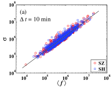
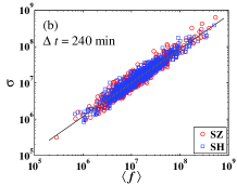
Figure 1: (color online) Scaling of capital flux fluctuations of the companies listed on the SZSE (open circles) and the SHSE (open squares) in the Chinese stock market. Panel (a) shows the dependence of the dispersions on the average capital fluxes for $\Delta t=10$ min, in which each point stands for a company. The power-law behavior between $\sigma_{i}^{10}$ and $\langle f_{i}^{10}\rangle$ is over 3 orders of magnitude with $\alpha^{10}=0.903\pm 0.007$. Panel (b) is the same as (a) but with a time scale of $\Delta t=240$ min (one trading day) and the scaling spans over 3 orders of magnitude with $\alpha^{240}=0.934\pm 0.007$.

These $\alpha$ values are different from $\alpha=0.5$ (endogenous driven systems) and $\alpha=1$ (exogenous driven systems) deMenezes-Barabasi-2004a-PRL ; deMenezes-Barabasi-2004b-PRL ; Barabasi-deMenezes-Balensiefer-Brockman-2004-EPJB . Kertész and Eisler point out system with inhomogeneous impact will induce scaling exponents $0.5<\alpha<1$ Kertesz-Eisler-2005a-XXX ; Kertesz-Eisler-2005b-XXX . However, the corresponding $\alpha$ value of the Chinese stock market is much larger than that of the American market at the same time scale. For instance, $\alpha\approx 0.88$ for the Chinese stock market while $\alpha\approx 0.73$ for the NYSE for $\Delta t=2$ min Kertesz-Eisler-2005a-XXX . The results imply that there are much more exogenous driving forces in the Chinese stock market than in the American market.

Figure 2 shows the dependence of the scaling exponent $\alpha^{\Delta t}$ with respect to the time scale $\Delta t$. We find that $\alpha^{\Delta t}$ increases linearly with the logarithm of the time scale $\Delta t$,

$$\alpha^{\Delta t}=\alpha^{*}+\gamma_{\alpha}\log\Delta t~{}.$$ (3)

A linear least squares regression gives the slope $\gamma_{\alpha}=0.0101\pm 0.0002$. According to the Efficient Market Hypothesis Fama-1970-JF ; Fama-1991-JF , the longer the information (news) spreads on the market, the more it is interpreted and digested by the market. Therefore, the market is more sensitive to exogenous driving forces than endogenous forces at large time scale. That’s the reason why $\alpha^{\Delta t}$ increases with $\Delta t$. For comparison, we also calculated the exponent $\alpha$ for the shuffled data. As is shown in Figure 2, the exponent $\alpha$ remains constant with respect to the time scale $\Delta t$, indicating that the correlations in the traded value series act at least as a key factor causing the equation (3).

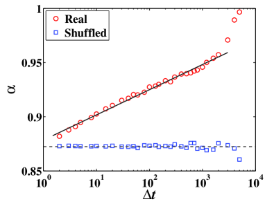
Figure 2: (color online) Dependence of the scaling exponent $\alpha$ on the time scale $\Delta t$. The open circles represent the real data, while the open squares are for the shuffled data for comparison.

3 Separating endogenous and exogenous dynamics

The macroscopic properties of complex systems may stem from the endogenous interactions between the elements in systems or the exogenous shocks from the environment or both. It is important to distinguish the endogenous and exogenous components of the system’s dynamic behaviors. de Menezes and coworkers have proposed a technique to separate endogenous and exogenous dynamics of complex systems deMenezes-Barabasi-2004b-PRL ; Barabasi-deMenezes-Balensiefer-Brockman-2004-EPJB . The observed dynamics of the capital fluxes are caused by the interplay between the endogenous and exogenous driving forces so that the observable can be written as the sum of two components:

$$f_{i}(t)=f_{i}^{\rm{exo}}(t)+f_{i}^{\rm{endo}}(t),$$ (4)

where $f_{i}(t)$ stands for the total capital flow, $f_{i}^{\rm{exo}}(t)$ represents the component due to exogenous driving forces, and $f_{i}^{\rm{endo}}(t)$ is endogenous component.

In the framework of de Menezes et al. deMenezes-Barabasi-2004b-PRL ; Barabasi-deMenezes-Balensiefer-Brockman-2004-EPJB , $f_{i}^{\rm{exo}}(t)$ is the product of the proportional coefficient $A_{i}$ and the total flux of the system at time $t$ (i.e. $\sum_{i=1}^{N}f_{i}(t)$). The coefficient $A_{i}$ is the ratio of the total cash flow of company $i$ during the period under investigation to the total trading capital flux of all the companies at the same time interval. Mathematically, we have

$$f_{i}^{\rm{exo}}(t)=A_{i}\sum_{i=1}^{N}f_{i}(t)~{},$$ (5)

where

$$A_{i}=\frac{\sum_{t=1}^{T}f_{i}(t)}{\sum_{t=1}^{T}\sum_{t=1}^{N}f_{i}(t)}~{}.$$ (6)

Combining Equations (4-6), it follows that,

$$f_{i}^{\rm{endo}}(t)=f_{i}(t)-\left[\frac{\sum_{t=1}^{T}f_{i}(t)}{\sum_{t=1}^{T}\sum_{t=1}^{N}f_{i}(t)}\right]\sum_{i=1}^{N}f_{i}(t)~{}.$$ (7)

By definition, we have $\langle f_{i}^{\rm{endo}}\rangle=0$.

Following the aforementioned approach, we are able to separate the exogenous and endogenous flux components from the total capital flows. We performed the analysis for different values of $\Delta{t}$ ranging from 2 min to 4500 min. The time evolution of the total capital flux with $\Delta{t}=2$ min of a typical stock and its resultant endogenous and exogenous components are illustrated in Figure 3. The results are qualitatively the same for other stocks and other time scales. It is interesting to observe that the endogenous component $f_{i}^{\rm{endo}}(t)$ exhibits high-frequency fluctuations while the exogenous component $f_{i}^{\rm{exo}}(t)$ shows low-frequency patterns. Specifically, $f_{i}^{\rm{exo}}(t)$ has sound intraday patterns with a period of half a day, which is reminiscent of the similar intraday pattern reported for the bid-ask spread of stocks in the Chinese market Gu-Chen-Zhou-2007-EPJB . We note that the Chinese stock market operates in the morning and in the afternoon with a closure from 11:30 to 13:00 in the noon.

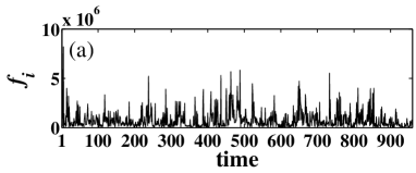
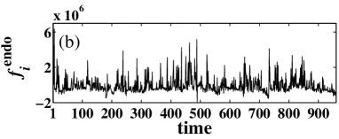
Figure 3: Separating the endogenous and exogenous contributions from the total capital fluxes. Panel (a) is the total capital flux, panel (b) is the endogenous component, and panel (c) is the exogenous component. There are evident intraday patterns in the exogenous signal.

The power-law scaling (1) also holds for the two components extracted. The scaling behaviors of the endogenous and exogenous fluctuations of the stocks traded in the the SHSE (open squares) and the SZSE (open circles) are presented in Figure 4(a) for time scale $\Delta t=10$ min and in Figure 4(b) for time scale $\Delta t=240$ min. All the scaling ranges span over more than three orders of magnitude. For $\Delta t=10$ min, the exogenous scaling exponent is $\alpha^{\rm{exo}}=1$ and the endogenous exponent is $\alpha^{\rm{endo}}=0.878\pm 0.008$. For $\Delta t=240$ min (one trading day), we have $\alpha^{\rm{exo}}=0.999\pm 0.0004$ and $\alpha^{\rm{endo}}=0.884\pm 0.009$. It is interesting to notice that the scaling relations of the exogenous components are less dispersed.

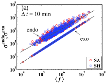
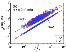
Figure 4: (color online) Power-law scaling of the endogenous and exogenous fluctuations with respect to the averages of the two components of stocks listed on the SHSE (open squares) and the SZSE (open circles) in the Chinese market. Panel (a) is for $\Delta t=10$ min. The exogenous scaling exponent is $\alpha^{\rm{exo}}=1$ and the endogenous exponent is $\alpha^{\rm{endo}}=0.878\pm 0.008$. Panel (b) is for $\Delta t=240$ min (one trading day), where $\alpha^{\rm{exo}}=0.999\pm 0.0004$ and $\alpha^{\rm{endo}}=0.884\pm 0.009$. The exogenous signals are shifted vertically for better visibility.

Figure 5 shows the dependence of the endogenous exponents $\alpha^{\rm{endo}}$ and the exogenous exponents $\alpha^{\rm{exo}}$ with respect to the time scale $\Delta{t}$. We find that, all the exogenous fluctuations $\sigma^{\rm{exo}}$ have the same scaling exponent $\alpha^{\rm{exo}}\approx 1$ at different time scales, while the scaling exponent of the endogenous fluctuations $\sigma^{\rm{endo}}$ almost remains constant with minor variations along the time scale $\Delta{t}$: $\alpha^{\rm{endo}}\approx 0.86\sim 0.89$. The fact that $\alpha^{\rm{endo}}$ is independent of $\Delta{t}$ is completely different from the resulting endogenous exponents reported for the NYSE case, where the endogenous exponent varies with the time scale Eisler-Kertesz-Yook-Barabasi-2005-EPL . The underlying mechanism of such discrepancy between the American market and the Chinese market is unclear. Possible causes include the absence of market orders, no short positions, the maximum percentage of fluctuation (10%) in each day, and the $t+1$ trading mechanism in the Chinese stock market on the one hand and the hybrid trading system containing both specialists and limit-order traders in the NYSE on the other hand.

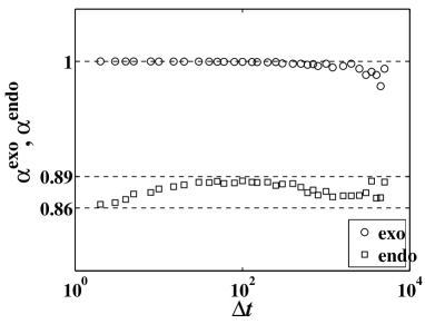
Figure 5: Dependence of the endogenous and exogenous scaling exponents $\alpha^{\rm{endo}}$ and $\alpha^{\rm{exo}}$ on the time scale $\Delta t$.

Utilizing the separated exogenous and endogenous signals, we can obtain the ratio of the exogenous dispersion to the endogenous dispersions as follows

$$\eta_{i}=\frac{\sigma_{i}^{\rm{exo}}}{\sigma_{i}^{\rm{endo}}}~{}.$$ (8)

When $\eta_{i}\gg 1$, the system is driven by exogenous factors. In contrast, the system is dominated by endogenous dynamics when $\eta_{i}\ll 1$. The empirical probability density distributions $p(\eta)$ for two typical time scales are shown in Figure 6 using histograms. One can see that the ratio $\eta_{i}$ has unimodal distribution. In addition, it is clearly visible that the $p(\eta)$ distributions observed at different time scales are different, indicating the dynamics of the system evolves with time scale $\Delta t$. For time scale $\Delta t=10$ min, the distribution is centered roughly around $\eta=0.5$ and no value of $\eta$ is larger than $1$, as suggested by Figure 6(a). This means that the dynamics at small time scale is dominated by endogenous driving forces. When the time scale increases to $\Delta=240$ min, the peak of the ratio distribution moves to around $\eta=0.8$ and some values of $\eta$ become larger than $1$ as shown in Figure 6(b), indicating that exogenous fluctuations have more impact on the system’s dynamics.

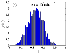
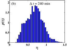
Figure 6: Empirical distribution of $\eta_{i}=\sigma_{i}^{\rm{exo}}/\sigma_{i}^{\rm{endo}}$ ratios of endogenous and exogenous fluctuations for two typical time scales $\Delta t=10$ min (a) and $\Delta t=240$ min (b).

We investigated the ratio $\eta$ at different time scales. For each time scale, we calculated the mean $\langle\eta\rangle$ of all the ratios of the 1354 stocks. Figure 7 presents the mean $\langle\eta\rangle$ of the ratios $\eta_{i}=\sigma_{i}^{\rm{exo}}/\sigma_{i}^{\rm{endo}}$ as a function of time scale $\Delta t$. The $\langle\eta\rangle$ function exhibits a clear upwards trend, increasing with $\Delta{t}$ from small values far less than 1 to large values much greater than 1. This trend hallmarks the crossover of relative competition of the endogenous dynamics and the exogenous dynamics of the Chinese stock market. This phenomenon confirms that the exogenous diving forces become stronger with the increasing of the time interval $\Delta t$ in stock markets Eisler-Kertesz-Yook-Barabasi-2005-EPL . When $\Delta t\geq 1800$ min (about $7.5$ trading days), $\langle\eta\rangle>1$, suggesting that the exogenous fluctuations overcome the endogenous ones and become the dominating factor effecting the system’s behaviors.

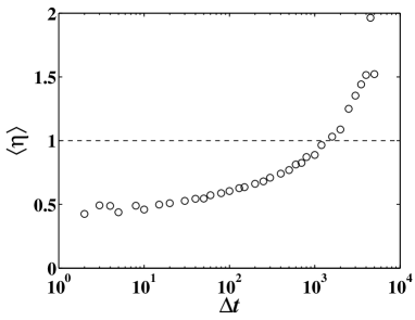
Figure 7: Mean of the ratios $\eta_{i}=\sigma_{i}^{\rm{exo}}/\sigma_{i}^{\rm{endo}}$ as a function of the time scale $\Delta t$.

4 Long memory in traded value time series

The temporal correlations have been extensively discussed in many physical and financial time series Bouchaud-Potters-2000 ; Mantegna-Stanley-2000 ; Sornette-2003 . There are many methods proposed for this purpose Taqqu-Teverovsky-Willinger-1995-Fractals ; Montanari-Taqqu-Teverovsky-1999-MCM , such as spectral analysis, rescaled range analysis Hurst-1951-TASCE ; Mandelbrot-Ness-1968-SIAMR ; Mandelbrot-Wallis-1969a-WRR ; Mandelbrot-Wallis-1969b-WRR ; Mandelbrot-Wallis-1969c-WRR ; Mandelbrot-Wallis-1969d-WRR , fluctuation analysis Peng-Buldyrev-Goldberger-Havlin-Sciortino-Simons-Stanley-1992-Nature , detrended fluctuation analysis (DFA) Peng-Buldyrev-Havlin-Simons-Stanley-Goldberger-1994-PRE ; Hu-Ivanov-Chen-Carpena-Stanley-2001-PRE ; Kantelhardt-Zschiegner-Bunde-Havlin-Bunde-Stanley-2002-PA , wavelet transform module maxima (WTMM) Holschneider-1988-JSP ; Muzy-Bacry-Arneodo-1991-PRL ; Muzy-Bacry-Arneodo-1993-JSP ; Muzy-Bacry-Arneodo-1993-PRE ; Muzy-Bacry-Arneodo-1994-IJBC , and detrended moving average Alessio-Carbone-Castelli-Frappietro-2002-EPJB ; Carbone-Castelli-Stanley-2004-PA ; Carbone-Castelli-Stanley-2004-PRE ; Alvarez-Ramirez-Rodriguez-Echeverria-2005-PA ; Xu-Ivanov-Hu-Chen-Carbone-Stanley-2005-PRE , to list a few. We adopt the fluctuation analysis to extract the Hurst exponent Eisler-Kertesz-2006-PRE ; Eisler-Kertesz-2006-EPJB ; Eisler-Kertesz-2006a-XXX ; Eisler-Kertesz-2006b-XXX ; Eisler-Kertesz-2006c-XXX ,

$$\sigma_{i}^{2}=\left\langle(f_{i}^{\Delta t}(t)-\langle f_{i}^{\Delta t}(t)\rangle)^{2}\right\rangle\sim\Delta t^{2H_{i}}~{}.$$ (9)

The Hurst exponent $H_{i}>0.5$ means that the time series is correlated, $H_{i}<0.5$ means that the time series is anti-correlated, and for $H_{i}=0.5$, it is uncorrelated.

Figure 8 shows the fluctuation analysis on the capital flux time series of two stocks: Wanke (Code 000002, circles) from the SZSE and Shanggang (Code 600018, squares) from the SHSE. The solid lines are the linear fits to the data, which give the Hurst exponents $H_{i}=0.863\pm 0.003$ for Wanke and $H_{i}=0.843\pm 0.007$ for Shanggang. The fact that the Hurst exponents of the two companies are much lager than 0.5 suggests that there is long-range memory in the traded values of individual companies. For comparison, we reshuffled the two data sets and performed the same fluctuation analysis. we obtain that $H_{i}=0.512\pm 0.005$ for the shuffled data of Wanke and $H_{i}=0.524\pm 0.007$ for the shuffled data of Shanggang, which are close to $H=0.5$. We stress that, according to Figure 8, there is no evident crossover of scaling regimes in the Chinese market. In contrast, there is a clear crossover behavior from uncorrelated regime when $\Delta{t}<t_{\times}$ to strongly correlated regime when $\Delta{t}>t^{\times}$ where $t_{\times}=20$ min and $t^{\times}=300$ min for the NYSE stocks and $t_{\times}=2$ min and $t^{\times}=60$ min for the NASDAQ stocks Eisler-Kertesz-2006-PRE ; Eisler-Kertesz-2006-EPJB ; Eisler-Kertesz-2006a-XXX ; Eisler-Kertesz-2006b-XXX ; Eisler-Kertesz-2006c-XXX .

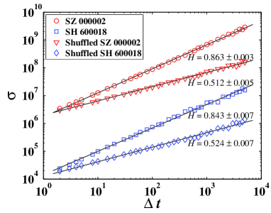
Figure 8: (color online) Fluctuation analysis on the capital flux time series of two stocks: Wanke (Code 000002, $\circ$) from the SZSE and Shanggang (Code 600018, $\square$) from the SHSE. The two flatter curves are obtained from the shuffled data of Wanke ($\triangledown$) and Shanggang ($\diamond$). The data points for Shanggang are translated vertically downwards by 100 for clarity.

The Hurst exponents for all the 1354 stocks are estimated. In Figure 9, we present as open circles the resulting Hurst exponents for different values of $\langle f_{i}\rangle$ after (approximately) logarithmic binning. One finds that the Hurst exponents of the traded values increase with the logarithm of mean traded value per minute and is approximately linear

$$H_{i}=H^{*}+\gamma_{H}\log\langle f_{i}\rangle~{},$$ (10)

where the slope $\gamma_{H}=0.013\pm 0.001$. This linear relationship between $H_{i}$ and $\log\langle f_{i}\rangle$ was first reported by Eilser and Kertész for the NYSE and NASDAQ but with larger slopes: $\gamma_{H}=0.06$ for the NYSE and $\gamma_{H}=0.05$ for the NASDAQ Eisler-Kertesz-2006-PRE ; Eisler-Kertesz-2006-EPJB ; Eisler-Kertesz-2006a-XXX ; Eisler-Kertesz-2006b-XXX ; Eisler-Kertesz-2006c-XXX . As a reference, we find that the shuffled data give an uncorrelated Hurst exponent $H_{i}\approx 0.5$ independent of the traded values. A linear regression gives that $\gamma_{H}=0.003\pm 0.002\approx 0$. Since $f_{i}$ is a measure of the size or capitalization of a company listed on stock exchanges, the relation (10) implies that the trading activities of larger companies exhibit stronger correlations. Moreover, the Hurst exponents for all the Chinese stock investigated are significantly larger than $H=0.5$, while that in the American market are close to $H=0.5$ for small companies Eisler-Kertesz-2006-PRE ; Eisler-Kertesz-2006-EPJB ; Eisler-Kertesz-2006a-XXX ; Eisler-Kertesz-2006b-XXX ; Eisler-Kertesz-2006c-XXX .

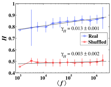
Figure 9: (color online) Linear dependence of the Hurst exponents $H$ on the average capital flux $\langle f\rangle$ for the real ($\circ$) and the shuffled data ($\square$).

There is an intriguing connection between the mean-variance relationship and the long memory nature of the capital flux time series. Combining (1) and (9), simple derivation leads to the following equality Eisler-Kertesz-2006-PRE

$$\gamma_{\alpha}=\frac{{\rm{d}}\alpha(\Delta t)}{{\rm{d}}(\log\Delta t)}=\frac{{\rm{d}}H_{i}}{{\rm{d}}(\log\langle f_{i}\rangle)}=\gamma_{H}~{}.$$ (11)

This relation is well verified by the American stock market data Eisler-Kertesz-2006-PRE . Our analysis in this work for the Chinese stock market gives further support to it. The evidence from the American and the China’s stock market are summarized in Table 1.

Table 1: Verification of the relation $\gamma_{\alpha}=\gamma_{H}$.

Stock market	NYSE	NASDAQ	China
$\gamma_{\alpha}$	$0.06\pm 0.01$	$0.06\pm 0.01$	$0.0101\pm 0.0002$
$\gamma_{H}$	$0.06\pm 0.01$	$0.05\pm 0.01$	$0.013~{}\pm 0.001~{}~{}$

5 Multiscaling and Multifractal analysis

The mean-variance analysis in equation (1) can be generalized to higher orders by utilizing the $q$-order central moments of the capital fluxes Eisler-Kertesz-Yook-Barabasi-2005-EPL ,

$$\sigma_{i}^{q}=\left\langle(f_{i}^{\Delta t}(t)-\langle f_{i}^{\Delta t}(t)\rangle)^{q}\right\rangle\sim\langle f_{i}\rangle^{q\alpha(q)}~{}.$$ (12)

where $q$ is a superscript in the term $\sigma_{i}^{q}$, not a power. When $q=2$, one recovers that $\sigma_{i}^{2}=(\sigma_{i})^{2}$. For $q<0$, equation (12) will enlarge the influences of the small fluctuations and reduce the effect of the large fluctuations, and vice versa.

The total and endogenous signals have been investigated through equation (12), and the power-law relations between the $q$-th order central moments of the signals and the mean total activities of the same component have been found as well. Figure 10 shows the multiscaling exponents $\alpha(q)$. It is found that $\alpha(q)$ also strongly depend on the time interval $\Delta t$ according to Figure 10. There are several differences between our results and that for the NYSE stocks Eisler-Kertesz-Yook-Barabasi-2005-EPL . First, the $\alpha(q)$ function for the Chinese market is larger than that of the NYSE market for same $q$ on average. This is maybe due to the fact that the Chinese market is more influenced by exogenous forces. Second, consider negative values of $q$. For $\Delta t=10$ min, $\alpha^{\rm{tot}}>\alpha^{\rm{endo}}$ in the Chinese market while $\alpha^{\rm{tot}}<\alpha^{\rm{endo}}$ in the NYSE market. For $\Delta{t}$ being a whole trading day, $\alpha^{\rm{tot}}<\alpha^{\rm{endo}}$ in the Chinese market, while $\alpha^{\rm{tot}}>\alpha^{\rm{endo}}$ in the NYSE market. Third, the difference between $\alpha^{\rm{tot}}$ and $\alpha^{\rm{endo}}$ is much larger in the Chinese market than in the NYSE market.

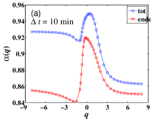
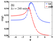
Figure 10: (color online). The multiscaling exponents $\alpha(q)$ as a a function of $q$ for $\Delta t=10$ min (a) and $\Delta t=240$ min (b).

Similarly, one can extend the fluctuation analysis in equation (9) to higher orders as follows Eisler-Kertesz-Yook-Barabasi-2005-EPL ,

$$\sigma_{i}^{q}=\left\langle(f_{i}^{\Delta t}(t)-\langle f_{i}^{\Delta t}(t)\rangle)^{q}\right\rangle\sim\Delta t^{\zeta_{i}(q)}~{},$$ (13)

which enables us to understand the multifractal nature of in the dynamics of the market. The relationship between the exponent $\zeta(q)$ and the generalized Hurst exponent $H(q)$ can be described as follows,

$$\zeta_{i}(q)=qH_{i}(q)~{}.$$ (14)

When $q=2$, $H_{i}=H_{(}2)$ is the Hurst exponent discussed in Section 4.

In order to have better statistics, we divided the 1354 stocks into 3 groups according to their average turnover $\langle f\rangle$: $10^{3}$ RMB/min $<\langle f\rangle\leq 10^{4}$ RMB/min, $10^{4}$ RMB/min $<\langle f\rangle\leq 10^{5}$ RMB/min, and $10^{5}$ RMB/min $<\langle f\rangle$. Note that $10^{3}$ RMB/min $<\langle f\rangle<10^{7}$ RMB/min for all stocks. The multifractal analysis is performed upon each individual group of stocks rather than individual stocks. The scaling of $\sigma^{q}$ is illustrated in Figure 11 for $q=-1$, $q=2$, $q=5$, and $q=8$. We can observe that there exist crossover regimes when the value of $q$ is large. Such crossover phenomena disappear for small values of $q$. This feature is again different from the NYSE case where crossover regimes are observed for all $q$ investigated Eisler-Kertesz-2006b-XXX . In the Chinese case, the crossover regime occurs with $\Delta t=40\sim 240$ min (one trading day).

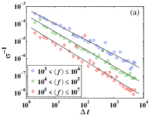
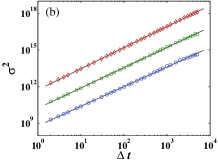
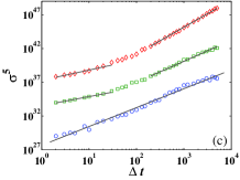
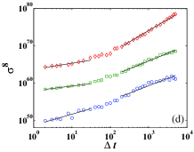
Figure 11: Plots of the partition function $\sigma^{q}$ as a function of the time scale $\Delta t$ for three groups of stocks and different $q$-th moments: (a) for $q=-1$, (b) for $q=2$, (c) for $q=5$, and (d) for $q=8$.

Figure 12 shows the scaling exponents $\zeta(q)$ as a function of powers of $q$. All the three $\zeta(q)$ function are nonlinear and concave showing that the three groups of stocks possess multifractal nature. Moreover, the group of companies with higher liquidity exhibit the stronger correlations, in agreement with the NYSE case Eisler-Kertesz-2006b-XXX .

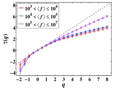
Figure 12: (color online) Dependence of the multifractal scaling exponents $\zeta(q)$ with respect to $q$-th order moments for three groups of companies.

6 Trading activities scaling with capitalization

Following the work of Zumbach Zumbach-2004-QF and Eisler and Kertétz’s Kertesz-Eisler-2005a-XXX ; Kertesz-Eisler-2005b-XXX ; Eisler-Kertesz-2006-EPJB , we investigate the scaling relationship between capitalization $M$, which ranges from $4.23\times 10^{8}$ to $6.33\times 10^{11}$ RMB, and the trading activities, which can be measured by the mean volume per trade $V$, the mean number of trades per minute $N$, and the mean turnover per minute $f$. The results are shown in Figure 13. Several power-law scaling are observed.

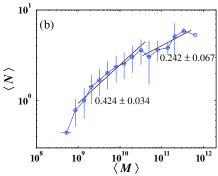
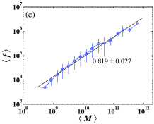
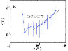
Figure 13: Scaling dependence between the measures of trading activities and capitalizations. (a) Mean volume per trade $V$ with respect to average capitalization $M$. (b) Mean number of trades per minute $N$ as a function of average capitalization $M$. (c) Mean turnover per minute $f$ versus the mean capitalization $M$. (d) Mean value per trade $V$ varying with mean number of trades per minute $N$.

The mean value per trade $V$ versus the capitalization $M$ is plotted in Figure 13(a), showing a significant power law scaling. The solid line is the best fit to the data for the whole regime, which gives a slope of $0.510\pm 0.015$. Figure 13(b) shows the dependence of the mean number of trades per minute $N$ with respect to the capitalization $M$. Least squares fits are performed for $6.3\times 10^{8}<M\leq 1.6\times 10^{10}$ and $M>1.6\times 10^{10}$ respectively, which give two exponents $0.424\pm 0.034$ and $0.242\pm 0.067$. The mean turnover per minute $f$ scales as a power law with respect to the mean capitalization $M$, as is suggested in Figure 13(c). The power law relation is spanned over three orders orders of magnitude, with a scaling exponent $0.819\pm 0.027$. These three plots indicate that the trade activities increase with the capitalization.

We further plot the mean volume per trade $V$ varying with mean number of trades per minute $N$ in Figure 13(d). Again a power law behavior for $N>1$ trades/min is observed,

$$\langle V_{i}\rangle=\langle N_{i}\rangle^{\beta}~{},$$ (15)

with $\beta=0.802\pm 0.075$. This behavior is also found in the FTSE-100 stocks with $\beta\approx 1$ Zumbach-2004-QF , in the NYSE stocks with $\beta=0.57\pm 0.09$ Kertesz-Eisler-2005b-XXX ; Eisler-Kertesz-2006-PRE ; Eisler-Kertesz-2006-EPJB , and in the NASDAQ stocks with $\beta=0.22\pm 0.04$ Eisler-Kertesz-2006-PRE . According to the “inhomogeneous impact” model, the exponent $\beta$ is related to the scaling exponent $\alpha$ as is expressed as follows Eisler-Kertesz-2005-PRE ; Eisler-Kertesz-2006-PRE

$$\alpha=\frac{1}{2}\left(1+\frac{\beta}{1+\beta}\right)~{}.$$ (16)

Substituting $\beta=0.802$ into equation (16), we obtain $\alpha=0.723$, which is much smaller than the actual value. This discrepancy might be due to the fact that $\beta$ is only found for larger stocks while $\alpha$ is obtained for all the stocks, and/or the inhomogeneous impact model, from which equation (16) is deduced, is too simplified for stock markets Eisler-Kertesz-2006a-XXX . Indeed, we find that the power-law scaling between $\langle{N}\rangle$ and $\langle{M}\rangle$ is not unambiguous. Suppose that $\langle{V}\rangle\sim\langle{M}\rangle^{\beta_{1}}$ and $\langle{N}\rangle\sim\langle{M}\rangle^{\beta_{2}}$. It follows immediately that $\langle{V}\rangle\sim\langle{N}\rangle^{\beta_{1}/\beta_{2}}$ such that $\beta=\beta_{1}/\beta_{2}$. This equality does not hold either in the Chinese stock market.

7 Conclusion

We have investigated the endogenous and exogenous dynamics of 1354 stocks traded in the Chinese stock market. These companies and the capital fluxes (proxied by traded values per unit time) among them are considered as a complex network. A non-universal scaling exponent $\alpha$ of fluctuations different from $1/2$ and $1$ is found with mean-variance analysis of the fluxes of different stocks. The scaling exponents at different time scales of the Chinese stocks are much larger than that of the NYSE stocks, suggesting that the Chinese market is influenced more heavily by the exogenous driving forces than the American market. The scaling exponent $\alpha$ increases linearly as the logarithm of time scale. The increasing of $\alpha$ also indicates that, for short time scale, the dynamics of the stock markets are dominated by endogenous fluctuations, while the exogenous fluctuations overcome the endogenous ones for large time scales. The fluxes signals can be separated into endogenous and exogenous components. Both components exhibit nice fluctuation scalings whose exponents $\alpha^{\rm{endo}}$ and $\alpha^{\rm{exo}}$ are independent of the time scale. The long memory existing in the capital flux time series is investigated by applying the fluctuation analysis. Our analysis on the Chinese stock market provides further evidence to the phenomenological observation that the Hurst exponent $H_{i}$ increases logarithmically with the mean capital flux $\langle f_{i}\rangle$. The empirical rule that $\gamma_{\alpha}=\gamma_{H}$ is verified.

We have also performed multiscaling analysis and multifractal analysis, as natural generalizations of the mean-variance analysis and the fluctuation analysis. The Chinese stock market exhibits multiscaling behavior and multifractal features. However, the multiscaling behavior and multifractal nature of the capital fluxes in the Chinese stock market are different in several aspects from that in the American market. The main difference is that crossover regime in the scalings is absent for small values of $q$ in the Chinese market.

In order to test the inhomogeneous impact model, the relationships among various measures of trading activities and capitalizations have been studied in the paper. A clearly power law behavior is found between the mean value per trade and the capitalization, as well as the mean capital flux and the capitalization. However, the interpretational power of the inhomogeneous impact model upon the Chinese stock market is not confirmed. Therefore, the underlying mechanism of the empirical observations is still open.

Acknowledgments:

This work was partially supported by the Fok Ying Tong Education Foundation (Grant No. 101086) and the Shanghai Rising-Star Program (Grant No. 06QA14015). We are grateful to Gao-Feng Gu and Guo-Hua Mu for the useful discussions.

References

- (1) K. Ziemelis, Nature 410, 241 (2001)
- (2) D. Sornette, Phys. World 12(12), 57 (1999)
- (3) D. Sornette, Proc. Natl. Acad. Sci. USA 99, 2522 (2002)
- (4) D. Sornette, Phys. Rep. 378, 1 (2003)
- (5) S. Albeverio, V. Jentsch, H. Kantz, eds., Endogenous versus exogenous origins of crises (Springer, Berlin, 2006)
- (6) D. Sornette, A. Helmstetter, Physica A 318, 577 (2003)
- (7) D. Sornette, Endogenous versus exogenous origins of crises, in Extreme Events in Nature and Society, edited by S. Albeverio, V. Jentsch, H. Kantz (Springer, Berlin, 2006), pp. 95–120
- (8) A. Johansen, D. Sornette, Physica A 276, 338 (2000)
- (9) A. Johansen, Physica A 296, 539 (2001)
- (10) A.G. Chessa, J.M.J. Murre, Physica A 333, 541 (2004)
- (11) D. Sornette, F. Deschatres, T. Gilbert, Y. Ageon, Phys. Rev. Lett. 93, 228701 (2004)
- (12) F. Deschatres, D. Sornette, Phys. Rev. E 72, 016112 (2005)
- (13) R. Lambiotte, M. Ausloos, Physica A 362, 485 (2006)
- (14) B.M. Roehner, D. Sornette, J.V. Andersen, International Journal of Modern Physics C 15, 809 (2004)
- (15) D. Sornette, Y. Malevergne, J.F. Muzy, Risk 16, 67 (2003)
- (16) A. Johansen, D. Sornette, in Contemporary Issues in International Finance (Nova Science Publishers, 2005), p. in press, (http://arXiv.org/abs/cond-mat/0210509)
- (17) D. Heymann, R.P.J. Perazzo, A.R. Schuschny, Adv. Complex Sys. 7, 21 (2004)
- (18) D. Sornette, W.X. Zhou, Physica A 370, 704 (2006)
- (19) W.X. Zhou, D. Sornette, Eur. Phys. J. B 54 (2006), physics/0503230
- (20) R. Albert, A.L. Barabási, Rev. Mod. Phys. 74, 47 (2002)
- (21) M.E.J. Newman, SIAM Rev. 45(2), 167 (2003)
- (22) S.N. Dorogovtsev, J.F.F. Mendes, Evolution of Networks: From Biological Nets to the Internet and the WWW (Oxford University Press, Oxford, 2003)
- (23) S. Boccaletti, V. Latora, Y. Moreno, M. Chavez, D.U. Hwang, Phys. Rep. 424, 175 (2006)
- (24) M.A. de Menezes, A.L. Barabási, Phys. Rev. Lett. 92, 028701 (2004)
- (25) M.A. de Menezes, A.L. Barabási, Phys. Rev. Lett. 93, 068701 (2004)
- (26) A.L. Barabási, M.A. de Menezes, S. Balensiefer, J. Brockman, Eur. Phys. J. B 38, 169 (2004)
- (27) L.R. Taylor, Nature 189, 732 (1961)
- (28) J.C. Nacher, T. Ochiai, T. Akutsu, Mod. Phys. Lett. B 19, 1169 (2005)
- (29) A. Mitnitski, K. Rockwood, Mech. Ageing Dev. 127, 70 (2006)
- (30) Z. Eisler, J. Kertész, S.H. Yook, A.L. Barabási, Europhys. Lett. 69, 664 (2005)
- (31) J. Kertész, Z. Eisler (2005), arXiv:physics/0503139
- (32) J. Kertész, Z. Eilser (2005), arXiv:physics/0512193
- (33) J. Živković, B. Tadić, N. Wick, S. Thurner, Eur. Phys. J. B 50, 255 (2006)
- (34) J. Duch, A. Arenas, Phys. Rev. Lett. 96, 218702 (2006)
- (35) Z. Eisler, J. Kertész, Phys. Rev. E 73, 046109 (2006)
- (36) Z. Eilser, J. Kertész, Eur. Phys. J. B 51, 145 (2006)
- (37) Z. Eilser, J. Kertész (2006), arXiv:physics/0603098
- (38) Z. Eilser, J. Kertész (2006), arXiv:physics/0606161
- (39) Z. Eilser, J. Kertész (2006), arXiv:physics/0608018
- (40) Z. Eisler, J. Kertész, Phys. Rev. E 71, 057104 (2005)
- (41) W.X. Zhou, D. Sornette, Physica A 337, 243 (2004)
- (42) G.F. Gu, W. Chen, W.X. Zhou, Eur. Phys. J. B p. submitted (2007), physics/0701017
- (43) D.W. Su, Chinese Stock Markets: A Research Handbook (World Scientific, Singapore, 2003)
- (44) E.F. Fama, J. Finance 25, 383 (1970)
- (45) E.F. Fama, J. Finance 46, 1575 (1991)
- (46) J.P. Bouchaud, M. Potters, Theory of Financial Risks: From Statistical Physics to Risk Management (Cambridge University Press, Cambridge, 2000)
- (47) R.N. Mantegna, H.E. Stanley, An Introduction to Econophysics: Correlations and Complexity in Finance (Cambridge University Press, Cambridge, 2000)
- (48) D. Sornette, Why Stock Markets Crash: Critical Events in Complex Financial Systems (Princeton University Press, Princeton, 2003)
- (49) M. Taqqu, V. Teverovsky, W. Willinger, Fractals 3, 785 (1995)
- (50) A. Montanari, M.S. Taqqu, V. Teverovsky, Math. Comput. Modell. 29(10-12), 217 (1999)
- (51) H.E. Hurst, Transactions of the American Society of Civil Engineers 116, 770 (1951)
- (52) B.B. Mandelbrot, J.W. Van Ness, SIAM Rev. 10, 422 (1968)
- (53) B.B. Mandelbrot, J.R. Wallis, Water Resour. Res. 5, 228 (1969)
- (54) B.B. Mandelbrot, J.R. Wallis, Water Resour. Res. 5, 242 (1969)
- (55) B.B. Mandelbrot, J.R. Wallis, Water Resour. Res. 5, 260 (1969)
- (56) B.B. Mandelbrot, J.R. Wallis, Water Resour. Res. 5, 967 (1969)
- (57) C.K. Peng, S.V. Buldyrev, A.L. Goldberger, S. Havlin, F. Sciortino, M. Simons, H.E. Stanley, Nature 356, 168 (1992)
- (58) C.K. Peng, S.V. Buldyrev, S. Havlin, M. Simons, H.E. Stanley, A.L. Goldberger, Phys. Rev. E 49, 1685 (1994)
- (59) K. Hu, P.C. Ivanov, Z. Chen, P. Carpena, H.E. Stanley, Phys. Rev. E 64, 011114 (2001)
- (60) J.W. Kantelhardt, S.A. Zschiegner, E. Koscielny-Bunde, S. Havlin, A. Bunde, H.E. Stanley, Physica A 316, 87 (2002)
- (61) M. Holschneider, J. Stat. Phys. 50, 953 (1988)
- (62) J.F. Muzy, E. Bacry, A. Arnéodo, Phys. Rev. Lett. 67, 3515 (1991)
- (63) J.F. Muzy, E. Bacry, A. Arnéodo, J. Stat. Phys. 70, 635 (1993)
- (64) J.F. Muzy, E. Bacry, A. Arnéodo, Phys. Rev. E 47, 875 (1993)
- (65) J.F. Muzy, E. Bacry, A. Arnéodo, Int. J. Bifur. Chaos 4, 245 (1994)
- (66) E. Alessio, A. Carbone, G. Castelli, V. Frappietro, Eur. Phys. J. B 27, 197 (2002)
- (67) A. Carbone, G. Castelli, H.E. Stanley, Physica A 344, 267 (2004)
- (68) A. Carbone, G. Castelli, H.E. Stanley, Phys. Rev. E 69, 026105 (2004)
- (69) J. Alvarez-Ramirez, E. Rodriguez, J.C. Echeverría, Physica A 354, 199 (2005)
- (70) L.M. Xu, P.C. Ivanov, K. Hu, Z. Chen, A. Carbone, H.E. Stanley, Phys. Rev. E 71, 051101 (2005)
- (71) G. Zumbach, Quant. Finance 4, 441 (2004)