A Quantitative Analysis of Measures of Quality in Science

Abstract

Condensing the work of any academic scientist into a one-dimensional measure of scientific quality is a difficult problem. Here, we employ Bayesian statistics to analyze several different measures of quality. Specifically, we determine each measure’s ability to discriminate between scientific authors. Using scaling arguments, we demonstrate that the best of these measures require approximately $50$ papers to draw conclusions regarding long term scientific performance with usefully small statistical uncertainties. Further, the approach described here permits the value-free (i.e., statistical) comparison of scientists working in distinct areas of science.

I Introduction

It appears obvious that a fair and reliable quantification of the ‘level of excellence’ of individual scientists is a near-impossible task adam:02 ; dellavalle:03 ; franck:99 ; adams:96 ; lehmann:06 . Most scientists would agree on two qualitative observations: (i) It is better to publish a large number of articles than a small number. (ii) For any given paper, its citation count—relative to citation habits in the field in which the paper is published—provides a measure of its quality. It seems reasonable to assume that the quality of a scientist is a function of his or her full citation record. The question is whether this function can be determined and whether quantitatively reliable rankings of individual scientists can be constructed. A variety of ‘best’ measures based on citation data have been proposed in the literature and adopted in practice raan:05 ; hirsch:05 . The specific merits claimed for these various measures rely largely on intuitive arguments and value judgments that are not amenable to quantitative investigation. (Honest people can disagree, for example, on the relative merits of publishing a single paper with $1000$ citations and publishing $10$ papers with $100$ citations each.) The absence of quantitative support for any given measure of quality based on citation data is of concern since such data is now routinely considered in matters of appointment and promotion which affect every working scientist.

Citation patterns became the target of scientific scrutiny in the 1960s as large citation databases became available through the work of Eugene Garfield garfield:77 and other pioneers in the field of bibliometrics. A surprisingly, large body of work on the statistical analysis of citation data has been performed by physicists. Relevant papers in this tradition include the pioneering work of D. J. de Solla Price, e.g. price:65 , and, more recently, redner:98 ; lehmann:03 ; hirsch:05 ; redner:05 . In addition, physicists are a driving force in the emerging field of complex networks. Citation networks represent one popular network specimen in which papers correspond to nodes connected by references (out-links) and citations (in-links). Citation networks have frequently been used as an example of growing networks with preferential attachment barabasi:99 . For reviews on this extensive subject, see albert:02 ; dorogovtsev:02 ; newman:03a . The aim of the present paper is to take such studies in a novel direction by addressing the question of which one-dimensional measure of citation data is best in a manner which is both quantitative and free of value judgments. Given the remarks above, the ability to answer this question depends on a careful definition of the word ‘best’.

The primary purpose of analyzing and comparing the citation records of individual scientists is to discriminate between them, i.e., to assign some measure of quality and its associated uncertainty to each scientist considered. Whatever the intrinsic and value-based merits of the measure, $m$, assigned to every author, it will be of no practical value unless the corresponding uncertainty, $\delta m$ is sufficiently small. From this point of view, the best choice of measure will be that which provides maximal discrimination between scientists and hence the smallest value of $\delta m$. We will demonstrate that the question of deciding which of several proposed measures is most discriminating, and therefore ‘best’, can be addressed quantitatively using standard statistical methods.

Although the approach is straightforward, it is useful first to describe it in general. We begin by binning all authors by some tentative measure, $m$, of the quality of their full citation record. The probability that an author will lie in bin $\alpha$ is denoted $p(\alpha)$. Similarly, we bin each paper according to the total number of citations. The full citation record for an author is simply the set $\{n_{i}\}$, where $n_{i}$ is the number of his/her paper in citation bin $i$. For each author bin, $\alpha$, we then empirically construct the conditional probability distribution, $P(i|\alpha)$, that a single paper by an author in this bin will lie in citation bin $i$. These conditional probabilities are the central ingredient in our analysis. They can be used to calculate the probability, $P(\{n_{i}\}|\alpha)$, that any full citation record was actually drawn at random on the conditional distribution, $P(i|\alpha)$ appropriate for a fixed author bin, $\alpha$. Bayes’ theorem allows us to invert this probability to yield

$$P(\alpha|\{n_{i}\})\sim P(\{n_{i}\}|\alpha)\,p(\alpha)\ ,$$ (1)

where $P(\alpha|\{n_{i}\})$ is the probability that the citation record $\{n_{i}\}$ was drawn at random from author bin $\alpha$. By considering the actual citation histories of authors in bin $\beta$, we can thus construct the probability $P(\alpha|\beta)$, that the citation record of an author initially assigned to bin $\beta$ was drawn on the the distribution appropriate for bin $\alpha$. In other words, we can determine the probability that an author assigned to bin $\beta$ on the basis of the tentative quality measure should actually be placed in bin $\alpha$. This allows us to determine both the accuracy of the initial author assignment its uncertainty in a purely statistical fashion.

While a good choice of measure will assign each author to the correct bin with high probability this will not always be the case. Consider extreme cases in where we elect to bin authors on the basis of measures unrelated to scientific quality, e.g., by hair/eye color or alphabetically. For such measures $P(i|\alpha)$ and $P(\{n_{i}\}|\alpha)$ will be independent of $\alpha$, and $P(\alpha|\{n_{i}\})$ will become proportional to prior distribution $p(\alpha)$. As a consequence, the proposed measure will have no predictive power whatsoever. It is obvious, for example, that a citation record provides no information of its author’s hair/eye color. The utility of a given measure (as indicated by the statistical accuracy with which a value can be assigned to any given author) will obviously be enhanced when the basic distributions $P(i|\alpha)$ depend strongly on $\alpha$. These differences can be formalized using the standard Kullback-Leibler divergence. As we shall see, there are significant variations in the predictive power of various familiar measures of quality.

The organization of the paper is as follows. Section II is devoted to a description of the data used in the analysis, Section III introduces the various measures of quality that we will consider. In Sections IV and V, we provide a more detailed discussion of the Bayesian methods adopted for the analysis of these measures and a discussion of which of these measures is best in the sense described above of providing the maximum discriminatory power. This will allow us in Section VI to address to the question of how many papers are required in order to make reliable estimates of a given author’s scientific quality; finally, Section A discusses the origin of asymmetries in some the measures. A discussion of the results and various conclusions will be presented in Section VII.

II Data

The analysis in this paper is based on data from the SPIRES database of papers in high energy physics. Our data set consists of all citable papers written by academic scientists from the theory subfield, ultimo 2003. All citations to papers outside of SPIRES were removed. In the context of this paper, we define an academic scientist as someone who has published $25$ papers or more. This definition is intended to include almost everyone with a permanent academic position and exclude those who leave academia early in their careers (and generally cease active journal publication) in the interests of maintaining the homogeneity of the data sample. For more see lehmann:03a , Chapters 3 and 4. The resulting data set includes $6\,737$ authors and a total of $274\,470$ papers. The actual number of papers is smaller than this since each multiple author paper is counted once per co-author. The theory subfield is, however, that part of high energy physics where this effect is least pronounced. This is due to the relatively small number of co-authors (typically $1-3$) per theoretical paper. In the case of the theory subfield, this weighting of papers by the number of co-authors has been shown to have negligible effects lehmann:03 .

The theory subsection of the SPIRES data has a power-law structure.

Figure 1: Logarithmically binned histogram of the citations counts of all papers by authors with more than $25$ publications in the theory subsection of SPIRES. The data is normalized and the axes are logarithmic.

Specifically the probability that a paper will recieve $k$ citations is approximately proportional to $(k+1)^{-\gamma}$ with $\gamma=1.11$ for $k\leq 50$ and $\gamma=2.78$ for $k>50$. The transition between these two power laws is found to be surprisingly sharp lehmann:03 . These features of the global distribution are also present in the conditional probabilities for sub-groups of authors binned according to most measures of quality. In virtually all cases, these conditional probabilities can also be described accurately by separate power laws in each of two regions with a relatively sharp transition between the regions. As one might expect, authors with more citations are described by flatter distributions (i.e., smaller values of $\gamma$) and a somewhat higher transition point. Figure 1 displays the total distribution of citations as a binned and normalized histogram.

Studies performed on the first $25$, first $50$ and all papers for a given value of $m$ show the absence of temporal correlations. It is of interest to see this explicitly.

Figure 2: Logarithmically binned histogram of the citations in bin $6$ of the median measure. The $\triangle$ points show the citation distribution of the first $25$ papers by all authors. The points marked by $\star$ show the distribution of citations from the first $50$ papers by authors who have written more than $50$ papers. Finally, the $\Box$ data points show the distribution of all papers by all authors. The axes are logarithmic.

Consider the following example. In Figure 2, we have plotted the distribution for bin $6$ of the median measure. There are $674$ authors in this bin. Two thirds of these authors have written $50$ papers or more. Only this subset is used when calculating the first $50$ papers results. In this bin, the means for the total, first 25 and first 50 papers are $11.3$, $12.8$, and $12.9$ citations per paper, respectively. The median of the distributions are $4$, $6$, and $6$. The plot in Figure 2 confirms these observations. The remaining bins and the other measures yield similar results.

Note that Figure 2 confirms the general observations on the shapes of the conditional distributions made above. Figure 2 also shows two distinct power-laws. Both of the power-laws in this bin are flatter than the ones found in the total distribution and the transition point is lower than in the total distribution from Figure 1.

III Measures of Scientific Excellence

Despite differing citation habits in different fields of science, most scientists agree that the number of citations of a given paper is the best objective measure of the quality of that paper. The belief underlying the use of citations as a measure of quality is that the number of citations to a paper provides an indication of how often the content of that paper has been used in the work of others. Note, however, the obvious fact that citations can only be interpreted as a meaningful proxy of quality relative to the citation habits of one’s peers or, put slightly differently, in the context of the citation habits of the field in which the paper is published. In lehmann:03 , we have shown that the theory subsection of SPIRES is indeed a very homogeneous data set. In this sense, we will assume that the citation count of a paper is a proxy of the intrinsic quality of that paper.

The questions remain, however, of how to extract a measure of the quality of an individual scientist from his citation record and how fairly to project this record onto a scalar measure. This question is non-trivial because the probability, $p(k)$ of finding a scientific paper with $k$ citations roughly follows an asymptotic power-law distribution, see Figs. 1 and 2. This fact was documented for the SPIRES data in Ref. lehmann:03 and holds true in many other scientific fields  price:65 ; redner:98 ; newman:03a . Thus, it is useful to consider some of the properties of the distribution of citations for all authors before discussing the various specific measures of quality to be considered here.

Empirical evidence indicates that most citation distributions are largely power-law distributed with $p(k)\sim k^{-\gamma}$. For small values of $k$, $\gamma\approx 1$; for larger values, $2<\gamma<3$. Although the average number of citations per paper is well-defined, the asymptotic power-law tails of these distributions cause their variance to be infinite. When the variance is not defined (or very large), the mean values of a finite sample fluctuate significantly as a function of sample size. As a consequence, the average number of citations, $\langle k\rangle$, in the citation record of a given author (which is precisely a finite sample drawn from a power-law probability distribution) is a potentially unreliable measure of the quality of an author’s citation record since the addition or removal of a single highly cited paper can materially alter an author’s mean. Nevertheless, the mean of an author’s citations is commonly used as an intensive scalar measure of author quality.

The reservations just expressed about the use of mean citations per paper apply with even greater force if one chooses to measure author quality by the number of citations of each author’s single most highly cited paper, $k_{\rm max}$. Virtually all of the stabilizing statistical power of the full citation record has been discarded, and even greater fluctuations can be expected in this measure as the sample size changes. In spite of such statistical arguments, there are reasons for considering the maximum cited paper as a measure of quality. It is perfectly tenable to claim that the author of a single paper with $1000$ citations is of greater value to science than the author of $10$ papers with $100$ citations each (even though the latter is far less probable than the former). In this sense, the maximally cited paper might provide better discrimination between authors of ‘high’ and ‘highest’ quality, and this measure merits consideration.

Another simple and widely used measure of scientific excellence is the average number of papers published by an author per year. This would be a good measure if all papers were cited equally. As we have just indicated, scientific papers are emphatically not cited equally, and few scientists hold the view that all published papers are created equal in quality and importance. Indeed, roughly 50% of all papers in SPIRES are cited $\leq 2$ times (including self-citation). This fact alone is sufficient to invalidate publication rate as a measure of scientific excellence. If all papers were of equal merit, citation analysis would provide a measure of industry rather than one of intrinsic quality.

In an attempt order to remedy this problem, Thomson Scientific (ISI) introduced the Impact Factor which is designed to be a “measure of the frequency with which the ‘average article’ in a journal has been cited in a particular year or period”. The Impact Factor can be used to weight individual papers. Unfortunately, citations to articles in a given journal also obey power-law distributions redner:05 . This has two consequences. First, the determination of the Impact Factor is subject to the large fluctuations which are characteristic of power-law distributions. Second, the tail of power-law distributions displaces the mean citation to higher values of $k$ so that the majority of papers have citation counts that are much smaller than the mean. This fact is for example expressed in the large difference between mean and median citations per paper. For the total SPIRES data base, the median is $2$ citations per paper; the mean is approximately $15$. Indeed, only $22\%$ of the papers in SPIRES have a number of citations in excess of the mean, cf. lehmann:03 . Thus, the dominant role played by a relatively small number of highly cited papers in determining the Impact Factor implies that it is subject to relatively large fluctuations and that it tends overestimate the level of scientific excellence of high impact journals. This fact was directly verified by Seglen seglen:94 , who showed explicitly that the citation rate for individual papers is uncorrelated to the impact factor of the journal in which it was published.

An alternate way to measure excellence is to categorize each author by the median number of citations of his papers, $k_{1/2}$. Clearly, the median is far less sensitive to statistical fluctuations since all papers play an equal role in determining its value. To demonstrate the robustness of the median, it is useful to note that the median of $\mathcal{N}=2N+1$ random draws on any normalized probability distribution, $q(x)$, is normally distributed in the limit $\mathcal{N}\to\infty$. To this end we define the integral of $q(x)$ as

$$Q(x)=\int^{x}q(x^{\prime})dx^{\prime}$$ (2)

Evidently, $Q(x)$ grows monotonically from $0$ to $1$ independent of $q(x)$. The ‘median’ of this sample is defined as that value of $x$ such that (i) one draw has the value $x$, (ii) $N$ draws have a value less than or equal to $x$, and (iii) $N$ draws have a value greater than or equal to $x$. The probability that the median is at $x$ is now given as

$$P_{x_{1/2}}(x)=\frac{(2N+1)!}{1!N!N!}q(x)Q(x)^{N}[1-Q(x)]^{N}\ .$$ (3)

For large $N$, the maximum of $P_{x_{1/2}}(x)$ occurs at $x=x_{1/2}$ where $Q(x_{1/2})=1/2$. Expanding $P_{x_{1/2}}(x)$ about its maximum value, we see that

$$P_{x_{1/2}}(x)=\frac{1}{\sqrt{2\pi\sigma^{2}}}\exp[-\frac{(x-x_{1/2})^{2}}{2\sigma^{2}}]\,,\qquad\sigma^{2}=\frac{1}{4q(x_{1/2})^{2}\mathcal{N}}\ .$$ (4)

A similar argument applies for every percentile. The statistical stability of percentiles suggests that they are well-suited for dealing with the power laws which characterize citation distributions.

Recently, Hirsch hirsch:05 proposed a different measure, $h$, intended to quantify scientific excellence. Hirsch’s definition is as follows: “A scientist has index $h$ if $h$ of his/her $N_{p}$ papers have at least $h$ citations each, and the other $(N_{p}-h)$ papers have fewer than $h$ citations each”hirsch:05 . Unlike the mean and the median, which are intensive measures largely constant in time, $h$ is an extensive measure which grows throughout a scientific career. Hirsch assumes that $h$ grows approximately linearly with an author’s professional age, defined as the time between the publication dates of the first and last paper. Unfortunately, this does not lead to an intensive measure. Consider, for example, the case of authors with large time gaps between publications, or the case of authors whose citation data are recorded in disjoint databases. A properly intensive measure can be obtained by dividing an author’s $h$-index by the number of his/her total publications. We will consider both approaches below.

The $h$-index represents an attempt to strike a balance between productivity and quality and to escape the tyranny of power law distributions which place strong weight on a relatively small number of highly cited papers. The problem is that Hirsch assumes an equality between incommensurable quantities. An author’s papers are listed in order of decreasing citations with paper $i$ having $C(i)$ citations. Hirsch’s measure is determined by the equality, $h=C(h)$, which posits an equality between two quantities with no evident logical connection. While it might be reasonable to assume that $h^{\gamma}\sim C(h)$, there is no reason to assume that $\gamma$ and the constant of proportionality are both $1$.

We will also include one intentionally nonsensical choice in the following analysis of the various proposed measures of author quality. Specifically, we will consider what happens when authors are binned alphabetically. In the absence of historical information, it is clear that an author’s citation record should provide us with no information regarding the author’s name. Binning authors in alphabetic order should thus fail any statistical test of utility and will provide a useful calibration of the methods adopted. The measures of quality described in this section are the ones we will consider in the remainder of this paper.

IV A Bayesian Analysis of Citation Data

The rationale behind all citation analyses lies in the fact that citation data is strongly correlated such that a ‘good’ scientist has a far higher probability of writing a good (i.e., highly cited) paper than a ‘poor’ scientist. Such correlations are clearly present in SPIRES  lehmann:03 ; lehmann:05 . We thus categorize each author by some tentative quality index based on their total citation record. Once assigned, we can empirically construct the prior distribution, $p(\alpha)$, that an author is in author bin $\alpha$ and the probability $P(N|\alpha)$ that an author in bin $\alpha$ has a total of $N$ publications. We also construct the conditional probability $P(i|\alpha)$ that a paper written by an author in bin $\alpha$ will lie in citation bin $i$. As we have seen earlier, studies performed on the first $25$, first $50$ and all papers of authors in a given bin reveal no signs of additional temporal correlations in the lifetime citation distributions of individual authors. In performing this construction, we have elected to bin authors in deciles. We bin papers into $L$ bins according to the number of citations. The binning of papers is approximately logarithmic (see Appendix A). We have confirmed that the results stated below are largely independent of the bin-sizes chosen.

We now wish to calculate the probability, $P(\{n_{i}\}|\alpha)$, that an author in bin $\alpha$ will have the full (binned) citation record $\{n_{i}\}$. In order to perform this calculation, we assume that the various counts $n_{i}$ are obtained from $N$ independent random draws on the appropriate distribution, $P(i|\alpha)$. Thus,

$$P(\{n_{i}\}|\alpha)=P(N|\alpha)N!\prod_{i=1}^{L}\frac{P(i|\alpha)^{n_{i}}}{(n_{i})!}\ .$$ (5)

Although large scale temporal correlations are known to be absent, transient correlations are possible. For example, one particularly well-cited paper could lead to an increased probability of high citations for its immediate successor(s). It is difficult to demonstrate their presence or absence, but the results of following section will provide a posteriori evidence that such correlations, if present, are not important.

(a) First initial	(b) Papers/year	(c) Hirsch (age)	(d) Hirsch (papers)
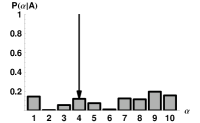
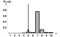
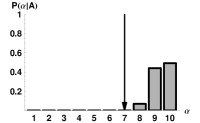
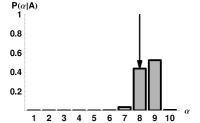
(e) Max	(f) Mean	(g) Median	(h) 65th percentile

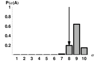
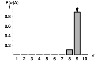
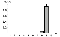
Figure 3: A single author example. We analyze the citation record of author $A$ with respect to the eight different measures defined in the text. Author $A$ has written a total of $88$ papers. The mean of this citation record is $26$ citations per paper, the median is $13$ citations, the $h$-index is $29$, the maximally cited paper has $187$ citations, and papers have been published at the average rate of $2.5$ papers per year. The various panels show the probability that author $A$ belongs to each of the ten deciles given on the corresponding measure; the vertical arrow displays the initial assignment. Panel (a) displays $P(\text{first initial}|A)$ (b) shows $P(\text{papers per year}|A)$, (c) shows $P(h/T|A)$, (d) shows $P(h/N|A)$, panel (e) shows $P(k_{\rm max}|A)$, panel (f) displays $P(\langle k\rangle|A)$, (g) shows $P(k_{1/2}|A)$ , and finally (h) shows $P(k_{.65}|A)$.

We can now invert the probability $P(\{n_{j}\}|\alpha)$ using Bayes’ theorem to obtain

$$P(\alpha|\{n_{i}\}) = \frac{P(\{n_{i}\}|\alpha)\,p(\alpha)}{P(\{n_{i}\})}$$ (6)

$$= \frac{p(\alpha)P(N|\alpha)\prod_{j}P(j|\alpha)^{n_{j}}}{\sum_{\beta}p(\beta)P(N|\beta)\,\prod_{k}P(k|\beta)^{n_{k}}}\ ,$$

where we have inserted Eq. (5) and used marginalization to obtain the normalization. The combinatoric factors cancel. The quantity $P(\alpha|\{n_{i}\})$, which represents the probability that an author with binned citation record $\{n_{i}\}$ is in author bin $\alpha$. It can be used in two ways—each of which is interesting.

For any measure chosen Eq. (6) provides us with the probability that an author lies in author bin $\alpha$. While the value of any measure (such as the mean number of citations per paper) can be calculated directly, the calculated values of $P(\alpha|\{n_{i}\})$ provide far more detailed and more reliable information using all statistical information contained in the data. The large fluctuations which can be encountered in identifying authors by their mean citation rate or by their maximally cited paper are reduced. Further, by providing us with values of $P(\alpha|\{n_{i}\})$ for all $\alpha$, we obtain a statistically trustworthy gauge of whether the resulting uncertainties in $\alpha$ are sufficiently small for the measure under consideration to be a reliable indicator of author quality. In short, Eq. (6) provides us with a measure of an author’s ranking independent of the total number papers currently published, and with information which allows us to assess the reliability of this determination. The accuracy of the resulting value of $\alpha$ increases dramatically with the total number of published papers. We will return to this point in Section V.

Fig. 3 shows the probabilities $P(\alpha|\{n_{i}\})$ that $A$ will lie in each of the decile bins using the measures discussed in section II. These measures include: (a) the first initial of the author’s name, (b) the average yearly output of papers, (c) Hirsch’s $h$ normalized by the author’s professional age $T$, (d) the $h$-index normalized by the number of published papers, (e) the citation count of the single most cited paper, (f) the mean number of citations per paper, (g) the median number (50th percentile) of citations per paper, and (h) a 65th percentile measure. It is clear from the figure that there are significant differences, both in the accuracy of of the initial assignments and, more importantly, in the corresponding uncertainties. Large uncertainties are due to the fact that the conditional probabilities, $P(i|\alpha)$ are largely independent of $\alpha$. Such independence is to be expected in the case of the alphabetic binning of authors, where the inability of the citation record to identify the first initial of author $A$’s name is hardly surprising. The figure also suggests that the number of papers published per year is not reliable. Initial assignments of author $A$ based on mean, median, 65th percentile, and maximum citations all appear to provide an accurate reflection of his full citation record with a satisfactorily small uncertainty. Hirsch’s measures falls somewhere between the best and worst choice of measures.

Given the large variations in the accuracy and confidence of decile assignments as a function of the measure selected, it is of interest to investigate in greater detail the question of which of these measures is best. We address this question in the next section.

V Weighing the Measures

In order to obtain a more graphic representation of the quality of a given measure, we calculate the probability, $P(\beta|\alpha)$, that an author initially assigned to bin $\alpha$ is predicted to lie in bin $\beta$. In practice, we determine $P(\beta|\alpha)$ as the average of the probability distributions $P(\beta|\{n_{i}\})$ for each author in bin $\alpha$. The results are shown ‘stacked’ in Fig. 4 for the various measures considered. Here, row $\alpha$ shows the (average) probabilities that an author initially assigned to bin $\alpha$ belongs in decile bin $\beta$. This probability is proportional to the area of the corresponding squares. Obviously, a perfect measure would place all of the weight in the diagonal entries of these plots. Weights should be centered about the diagonal for an accurate identification of author quality and the certainty of this identification grows as weight accumulates in the diagonal boxes. Note that an assignment of a decile based on Eq. (6) is likely to be more reliable than the value of the initial assignment since the former is based on all information contained in the citation record.

(a) First Initial	(b) Papers/year	(c) Hirsch (age)	(d) Hirsch (papers)
(e) Max	(f) Mean	(g) Median	(h) 65th percentile

Figure 4: Eight different measures. Each horizontal row shows the average probabilities (proportional to the areas of the squares) that authors initially assigned to decile bin $\alpha$ are predicted to belong in bin $\beta$. Panels as in Fig. 3.

Figure 4 emphasizes that ‘first initial’ and ‘publications per year’ are not reliable measures. The $h$-index normalized by professional age performs poorly; when normalized by number of papers, the trend towards the diagonal is enhanced. We note the appearance of vertical bars in each figure in the top row. This feature is explained in Appendix A. All four measures in the bottom row perform fairly well. The initial assignment of the $k_{\rm max}$ measure always underestimates an author’s correct bin. This is not an accident and merits comment. Specifically, if an author has produced a single paper with citations in excess of the values contained in bin $\alpha$, the probability that he will lie in this bin, as calculated with Eq. (6), is strictly $0$. Non-zero probabilities can be obtained only for bins including maximum citations greater than or equal to the maximum value already obtained by this author. (The fact that the probabilities for these bins shown in Fig. 4 are not strictly $0$ is a consequence of the use of finite bin sizes.) Thus, binning authors on the basis of their maximally cited paper necessarily underestimates their quality. The mean, median and 65th percentile appear to be the most balanced measures with roughly equal predictive value.

It is clear from Eq. (6) that the ability of a given measure to discriminate is greatest when the differences between the conditional probability distributions, $P(i|\alpha)$, for different author bins are largest. These differences can quantified by measuring the ‘distance’ between two such conditional distributions with the aid of the Kullback-Leibler (KL) divergence (also know as the relative entropy). The KL divergence between two discrete probability distributions, $p$ and $p^{\prime}$ is defined as

$$\mathrm{KL}[p,p^{\prime}]=\sum_{i}p_{i}\ln\left(\frac{p_{i}}{p_{i}^{\prime}}\right).$$ (7)

The Kullback-Leibler divergence is positive and has desirable convexity properties. It is, however, not a metric due to the fact that $\mathrm{KL}[p^{\prime},p]\neq\mathrm{KL}[p,p^{\prime}]$. While this asymmetry is of little concern when the differences between $p$ and $p^{\prime}$ are small, some care is required when such differences are large. This can occur when the data set is so small that some citation bins are empty or when we bin authors by $k_{\rm max}$, in which case empty bins are inevitable as noted above.

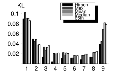
Figure 5: The Kullback-Leibler divergences $\mathrm{KL}[P(i|\alpha),P(i|\alpha+1)]$. Results are shown for the following distributions: $h$-index normalized by number of publications, maximum number of citations, mean, median, and 65th percentile.

We consider the KL distance between adjacent distributions, Fig. 5 shows the distances $\mathrm{KL}[P(i|\alpha),P(i|\alpha+1)]$ for various measures. The probability $P(\beta=\alpha+1|\alpha)$ is exponentially sensitive to the KL divergence. Measures with large KL divergences between adjacent bins provide the most certain assignments of authors. The KL divergences for the measures not shown are significantly smaller than those displayed. The results of Fig. 5 provide quantitative support for the roughly equal performance of mean, median, and 65th percentile measures seen in Figure 4. The $h$-index normalized by number of publications is dramatically smaller than the other measures shown except for the extreme deciles.

The reduced ability of all measures to discriminate in the middle deciles is immediately apparent from Fig. 5.

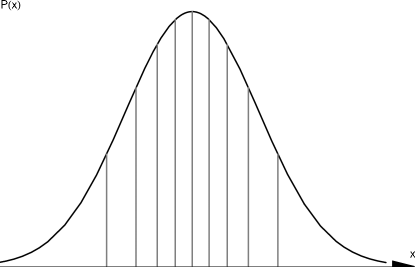
Figure 6: Binning according to deciles. This plot displays a normal distribution (solid black line) as an example of a probability distribution peaked around a non-zero maximum. The grey vertical lines mark the boundaries of the $10$ deciles.

This is a direct consequence any percentile binning given that the distribution of author quality has a maximum at some non-zero value, the bin size of a percentile distribution near the maximum will necessarily be small. The accuracy with which authors can be assigned to a given bin in the region around the maximum is reduced since one is attempting to distinguish between authors with very similar citation distributions. As a result, the statistical accuracy of percentile assignments is high at the extremes and relatively low in the middle of the distribution where we are attempting to make fine distinctions between scientists of similar ability. This effect is illustrated in Fig. 6.

VI Scaling

In this section, we consider the question of how many published papers are required in order to make a reliable prediction of the percentile ranking of a given author. (We consider results only using the 65th percentile measure.) If this number is sufficiently small, analysis along the lines presented here can provide a practical tool of potential value in predicting long-term scientific performance. In order to address this question, we will consider how $P(\alpha|\{n_{i}\})$ scales as a function of the total number of publications for an average author in each bin. Assume that an average author belonging to bin $\alpha$ draws $N$ papers at random from the distribution of $P(i|\alpha)$. The most probable number of papers in each citation bin will thus be given as $n_{i}=NP(i|\alpha)$. Inserting this result into Eq. (6) and discarding all fixed factors, we find that

$$P(\alpha|\{n_{i}\})\sim p(\alpha)\left(\prod_{i}P(i|\alpha)^{P(i|\alpha)}\right)^{N}\ .$$ (8)

For the same citation record, $\{n_{i}\}$, a similar expression permits determination of the probability that this average author will be assigned to any bin, $\beta$. We see that

$$\lim_{N\to\infty}\,\frac{1}{N}\,\ln\left(\frac{P(\beta|\{n_{i}\})}{P(\alpha|\{n_{i}\})}\right)=-\mathrm{KL}\left[P(\bullet|\alpha),P(\bullet|\beta)\right]\ .$$ (9)

This equation illustrates the utility of the KL divergence and explains the origin of its lack of symmetry. It is clear from Eqs. (8) and (9) that the probability of assigning this average author to the wrong bin will ultimately vanish exponentially with $N$. Given enough papers, the largest bin will ultimately dominate.

To obtain a quantitative sense of how many papers are required in practice, we pose the following question: What is the probability that a typical author

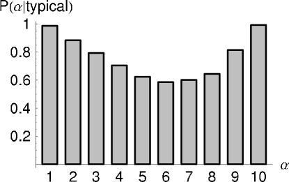
Figure 7: The probability that a typical (i.e., most probable) author with $50$ published papers will be assigned to the correct decile as a function of actual author decile. The median number of citations is used as a measure.

from each author decile with $N=50$ published papers will be assigned to the correct decile? The answer is plotted as a histogram in Fig. 7 using the 65th percentile citation rate as a measure (Similar results are obtained when using the mean or median citation rates). The figure indicates that $N=50$ papers is more than sufficient to identify authors in the first and tenth deciles. In fact, approximately $25$ and $20$ papers respectively are sufficient to place authors in these deciles at the 90% confidence level. Fig. 7 also indicates that $\approx 50$ published papers are sufficient to make meaningful assignments of authors to the second, third, and ninth deciles. All measures have difficulty in assigning authors to deciles $5-8$. As indicated by the small values of the KL divergence in these bins for all measures considered, the citation distributions of these authors are simply too similar to permit accurate discrimination (see arguments in the previous section). On the other hand, the probability that an author can be correctly assigned to one of these middle bins on the basis of $50$ publication is high. This difficulty is due to the relatively small range of citations ranges which cover these bins: the 65th percentile-bins 5 though 8 contain authors with a 65th percentile between 5 and 13 citations (cf. the narrow ranges of the middle bins in the case of the mean, displayed in Table 2).

VII Conclusions

There are two distinct questions which must be addressed in any attempt to use citation data as an indication of author quality. The first is whether the measure chosen to characterize a given citation distribution or even the citation distribution itself reflects the qualities that we would like to probe. The second question is whether a given measure is capable of discriminating between authors in a statistically reliable way and, by extension, which of several measures is best. We have shown that the use of Bayesian statistics and the Kullback-Leibler divergence can answer this question in a value-neutral and statistically compelling manner. It is possible to draw reliable conclusions regarding an author’s citation record on the basis of approximately 50 papers, and it is possible to assign meaningful statistical uncertainties to the results. The high level of discrimination obtained in the highest and lowest deciles provides indirect support for our assumption that an author’s citation record is drawn at random from an appropriate conditional distribution and suggests that possible additional correlations in citation data are not important. Further, the difficulty in discriminating between authors in the middle deciles suggests that intrinsic author ability is peaked at some non-zero value.

The probabilistic methods adopted here permit meaningful comparison of scientists working in distinct areas with only minimal value judgments. It seems fair, for example, to declare equality between scientists in the same percentile of their peer groups. It is similarly possible to combine probabilities in order to assign a meaningful ranking to authors with publications in several disjoint areas. All that is required is knowledge of the conditional probabilities appropriate for each homogeneous subgroup.

We note, however, that the number of publications required to make meaningful author assignments is large enough to limit the utility of such analyses in the academic appointment process. This raises the question of whether there are more efficient measures of an author’s full citation record than those considered here. Our object has been to find that measure which is best able to assign the most similar authors together. Straightforward iterative schemes can be constructed to this end and are found to converge rapidly (i.e., exponentially) to an optimal binning of authors. (The result is optimal in the sense that it maximizes the sum of the KL divergences, $KL[P(\bullet|\alpha),P(\bullet|\beta)]$, over all $\alpha$ and $\beta$.) The results are only marginally better than those obtained here with the mean, median or 65th percentile measures.

Finally, it is also important to recognize that it takes time for a paper to accumulate its full complement of citations. While their are indications that an author’s early and late publications are drawn (at random) on the same conditional distribution lehmann:03 , many highly cited papers accumulate citations at a constant rate for many years after their publication. This effect, which has not been addressed in the present analysis, represents a serious limitation on the value of citation analyses for younger authors. The presence of this effect also poses the additional question of whether there are other kinds of statistical publication data that can deal with this problem. Co-author linkages may provide a powerful supplement or alternative to citation data. (Preliminary studies of the probability that authors in bins $\alpha$ and $\beta$ will co-author a publication reveal a striking concentration along the diagonal $\alpha=\beta$.) Since each paper is created with its full set of co-authors, such information could be useful in evaluating younger authors. This work will be reported elsewhere.

Appendix A Vertical Stripes

The most striking feature of the calculated $P(\beta|\alpha)$ shown in Fig. 4 is presence of vertical ‘stripes’. These stripes are most pronounced for the poorest measures and disappear as the reliability of the measure improves. Here, we offer a schematic but qualitatively reliable explanation of this phenomenon. To this end, imagine that each author’s citation record is actually drawn at random on the true distributions $Q(i|A)$. For simplicity, assume that every author has precisely $N$ publications, that each author in true class $A$ has the same distribution of citations with $n_{i}^{A}=NQ(i|A)$, and that there are equal numbers of authors in each true author class. These authors are then distributed into author bins, $\alpha$, according to some chosen quality measure. The methods of Sections IV and V can then be used to determine $P(i|\alpha)$, $P(\{n_{i}^{(A)}\}|\beta)$, $P(\beta|\{n_{i}^{(A)}\})$ and $P(\beta|\alpha)$. Given the form of the $n_{i}^{(A)}$ and assuming that $N$ is large, we find that

$$P(\beta|\{n_{i}^{(A)}\})\approx\exp{\left(-N\mathrm{KL}[Q(\bullet|A),P(\bullet|\beta)]\right)}$$ (10)

and

$$\tilde{P}(\beta|\alpha)\sim\sum_{A}\,P(A|\alpha)\exp{\left(-N\mathrm{KL}[Q(\bullet|A),P(\bullet|\beta)]\right)}\ ,$$ (11)

where $P(A|\alpha)$ is the probability that the citation record of an author assigned to class $\alpha$ was actually drawn on $Q(i|A)$. The results of this approximate evaluation are shown in Fig. 8 and compared with the exact values of $P(\beta|\alpha)$ for the papers per year measure. The approximations do not affect the qualitative features of interest.

We now assume that the measure defining the author bins, $\alpha$, provides a poor approximation to the true bins, $A$. In this case, authors will be roughly uniformly distributed, and the factor $P(A|\alpha)$ appearing in Eq. (A2) will not show large variations. Significant structure will arise from the exponential terms, where the presence of the factor $N$ (assumed to be large), will amplify the differences in the KL divergences. The KL divergence will have a minimum value for some value of $A=A_{0}(\beta)$, and this single term will dominate the sum. Thus, $\tilde{P}(\beta|\alpha)$ reduces to

$$\tilde{P}(\beta|\alpha)\sim P(A_{0}|\alpha)\exp{\left(-N\mathrm{KL}[Q(\bullet|A_{0}),P(\bullet|\beta)]\right)}\ .$$ (12)

The vertical stripes prominent in Figs. 4(a) and (b) emerge as a consequence of the dominant $\beta$-dependent exponential factor.

(a) Papers/year $\tilde{P}(\alpha^{\prime}|\alpha)$	(b) Papers/year $P(\alpha^{\prime}|\alpha)$

Figure 8: A comparison of the approximate $\tilde{P}(\beta|\alpha)$ from Eq. (11) and the exact $P(\beta|\alpha)$ for the papers published per year measure.

The present arguments also apply to the worst possible measure, i.e., a completely random assignment of authors to the bins $\alpha$. In the limit of a large number of authors, $N_{\rm aut}$, all $P(i|\beta)$ will be equal except for statistical fluctuations. The resulting KL divergences will respond linearly to these fluctuations. These fluctuations will be amplified as before provided only that $N_{\rm aut}$ grows less rapidly than $N^{2}$. The argument here does not apply to good measures where there is significant structure in the term $P(A|\alpha)$. (For a perfect measure, $P(A|\alpha)=\delta_{A\alpha}$.) In the case of good measures, the expected dominance of diagonal terms (seen in the lower row of Fig. 4) remains unchallenged.

Appendix B Explicit Distributions

For convenience we present all data to determine the probabilities $P(\alpha|\{n_{i}\})$ for authors who publish in the theory sub-section of SPIRES. Data is presented only for case of the mean number of citations. All citations are binned logarithmically according to the citation bins listed in column one and two of Table 1.

$P(i|\alpha)$			$P(N|\alpha)$
Bin number	Citation range		Bin Number	Total paper range
$i=1$	$k$	$=1$	$m=1$	$N$	$=25$
$i=2$	$k$	$=2$	$m=2$	$N$	$=26$
$i=3$	$2<$ $k$	$\leq 4$	$m=3$	$26<$ $N$	$\leq 28$
$i=4$	$4<$ $k$	$\leq 8$	$m=4$	$28<$ $N$	$\leq 32$
$i=5$	$8<$ $k$	$\leq 16$	$m=5$	$32<$ $N$	$\leq 40$
$i=6$	$16<$ $k$	$\leq 32$	$m=6$	$40<$ $N$	$\leq 56$
$i=7$	$32<$ $k$	$\leq 64$	$m=7$	$56<$ $N$	$\leq 88$
$i=8$	$64<$ $k$	$\leq 128$	$m=8$	$88<$ $N$	$\leq 152\,$
$i=9$	$128<$ $k$	$\leq 256$	$m=9$	$\,152<$ $N$	$\leq N_{\rm max}$
$i=10$	$256<$ $k$	$\leq 512\,$
$i=11$	$\,512<$ $k$	$\leq k_{\rm max}$

Table 1: The binning of citations and total number of papers. The first and second column show the bin number and bin ranges for the citation bins used to determine the conditional citation probabilities $P(i|\alpha)$ for each $\alpha$, shown in Table 3. The third and fourth column display the bin number and total number of paper ranges used in the creation of the conditional probabilities $P(m|\alpha)$ for each $\alpha$, displayed in Table 4.

The author bins are determined on the basis of deciles of the total distribution of mean citations, $p(\langle k\rangle)$. Table 2 shows the relevant quantities for these bins.

$\alpha$	$\langle k\rangle$-range		# authors	$p(\alpha)$	$\bar{n}(\alpha)$
1	$0$ –	$1.69$	673	0.1	37.0
2	$1.69$ –	$3.08$	673	0.1	41.8
3	$3.08$ –	$4.88$	675	0.1	44.0
4	$4.88$ –	$6.94$	673	0.1	46.8
5	$6.94$ –	$9.40$	674	0.1	52.2
6	$9.40$ –	$12.56$	674	0.1	54.3
7	$12.56$ –	$16.63$	673	0.1	59.5
8	$16.63$ –	$22.19$	674	0.1	59.0
9	$22.19$ –	$33.99$	674	0.1	65.4
10	$\,\,33.99$ –	$285.88\,\,$	674	0.1	72.2

Table 2: The author bins. This table shows the mean numbers of citations that define the limits of the $10$ author bins.

Given the definitions of both the author- and citation bins, we can determine the conditional citation distributions $P(i|\alpha)$ empirically. These are given in Table 3.

	$i=1$	$i=2$	$i=3$	$i=4$	$i=5$	$i=6$	$i=7$	$i=8$	$i=9$	$i=10$	$i=11$
$\alpha=1$	0.612	0.182	0.127	0.057	0.019	0.002	0.000	0.000	0.000	0.000	0.000
$\alpha=2$	0.433	0.188	0.181	0.122	0.055	0.016	0.004	0.000	0.000	0.000	0.000
$\alpha=3$	0.327	0.165	0.188	0.167	0.103	0.038	0.010	0.002	0.000	0.000	0.000
$\alpha=4$	0.263	0.143	0.178	0.184	0.140	0.067	0.019	0.005	0.001	0.000	0.000
$\alpha=5$	0.217	0.127	0.163	0.183	0.165	0.096	0.036	0.009	0.002	0.000	0.000
$\alpha=6$	0.177	0.113	0.150	0.181	0.173	0.126	0.058	0.017	0.004	0.001	0.000
$\alpha=7$	0.143	0.098	0.135	0.170	0.183	0.149	0.086	0.028	0.007	0.002	0.000
$\alpha=8$	0.118	0.080	0.121	0.155	0.182	0.169	0.110	0.048	0.012	0.003	0.000
$\alpha=9$	0.094	0.066	0.099	0.141	0.175	0.178	0.139	0.075	0.025	0.007	0.001
$\alpha=10$	0.068	0.045	0.071	0.107	0.145	0.171	0.166	0.121	0.067	0.027	0.012

Table 3: The distributions $P(i|\alpha)$. This table displays the conditional probabilities that an author writes a paper in paper-bin $i$ given that his author-bin is $\alpha$.

We also need the probabilities $P(N|\alpha)$ describing that an author in bin $\alpha$ has $N$ publications. Because of the low number of authors in each bin, we need to bin the total number of publications when calculating this probability; we use the letter $m$ to enumerate the $N$-bins. Because $P(N|\alpha)$ is described by a power-law distribution and since we only consider authors with more than $25$ publications, we choose to bin $N$ logarithmically as displayed in the third and fourth column of Table 1. The conditional probabilities, $P(m|\alpha)$ are displayed in Table 4.

	$m=1$	$m=2$	$m=3$	$m=4$	$m=5$	$m=6$	$m=7$	$m=8$	$m=9$
$\alpha=1$	0.083	0.071	0.134	0.226	0.224	0.172	0.082	0.006	0.001
$\alpha=2$	0.058	0.049	0.103	0.187	0.236	0.217	0.122	0.025	0.003
$\alpha=3$	0.068	0.050	0.095	0.133	0.231	0.240	0.136	0.041	0.004
$\alpha=4$	0.043	0.049	0.095	0.141	0.198	0.247	0.162	0.061	0.004
$\alpha=5$	0.031	0.059	0.067	0.108	0.181	0.246	0.200	0.091	0.016
$\alpha=6$	0.031	0.039	0.068	0.126	0.162	0.245	0.215	0.099	0.015
$\alpha=7$	0.034	0.022	0.058	0.114	0.152	0.242	0.215	0.128	0.034
$\alpha=8$	0.028	0.024	0.049	0.096	0.178	0.243	0.248	0.101	0.033
$\alpha=9$	0.030	0.033	0.037	0.074	0.148	0.228	0.245	0.160	0.045
$\alpha=10$	0.027	0.028	0.043	0.077	0.131	0.212	0.199	0.223	0.061

Table 4: The conditional probabilities $P(m|\alpha)$. This table contains the conditional probabilities that an author has a total number of publications in publication-bin $m$ given that his author-bin is $\alpha$ .

References

- (1) D. Adam. The counting house. Nature, 415:726, 2002.
- (2) R. P. Dellavalle, E. J. Hester, L. F. Heilig, A. L. Drake, J. W. Kuntzman, M. Graber, and L. M. Schilling. Going, going, gone: Lost internet references. Science, 302:787, 2003.
- (3) G. Franck. Scientific communication – A vanity fair. Science, 286:53, 1999.
- (4) J. Adams and Z. Griliches. Measuring science: An exploration. Proceedings of the National Academy of Sciences, USA, 93:12664, 1996.
- (5) S. Lehmann, A. D. Jackson, and B. E. Lautrup. Measures for measures. Nature, 444:1003, 2006.
- (6) A. F. J. van Raan. Statistical properties of bibliometric indicators: Research group indicator distributions and correlations. Journal of the American Society for Information Science, 57:408, 2005.
- (7) J. E. Hirsch. An index to quantify an individual’s scientific output. Proceedings of the National Academy of the Sciences, 102:16569, 2005.
- (8) E. Garfield. Essays of an Information Scientist, volume 1-15. ISI Press, 1977-1993.
- (9) D. de Solla Price. Networks of scientific papers. Science, 149:510, 1965.
- (10) S. Redner. How popular is your paper? An emperical study of the citation distribution. European Physics Journal B, 4:131, 1998.
- (11) S. Lehmann, B. E. Lautrup, and A. D. Jackson. Citation networks in high energy physics. Physical Review E, 68, 2003.
- (12) S. Redner. Citation statistics from 110 years of physical review. Physics Today, 58:49, 2005.
- (13) A.-L. Barabási and R. Albert. Emergence of scaling in random networks. Science, 286:509, 1999.
- (14) R. Albert and A.-L. Barabási. Statistical mechanics of complex networks. Reviews of modern physics, 74:47, 2002.
- (15) S. N. Dorogovtsev and J. F. F. Mendes. Evolution of networks. Advances in Physics, 51:1079, 2002.
- (16) M. E. J. Newman. The structure and function of complex networks. SIAM Review, 45:167, 2003.
- (17) S. Lehmann. Spires on the building of science. Master’s thesis, The Niels Bohr Institute, 2003. May be downloaded from www.imm.dtu.dk/slj/.
- (18) M. V. Simkin and V. P. Roychowdhury. Read before you cite! Complex Systems, 14:269, 2003.
- (19) M. E. J. Newman. Power laws, pareto distributions and zipf’s law. Contemporary Physics, 46:323, 2005.
- (20) P. O. Seglen. Casual relationship between article citedness and journal impact. Journal of the American Society for Information Science, 45:1, 1994.
- (21) S. Lehmann, A. D. Jackson, and B. E. Lautrup. Life, death, and preferential attachment. Europhysics Letters, 69:298, 2005.
- (22) A. J. Lotka. The frequency distribution of scientific productivity. Journal of the Washington Academy of Sciences, 16:317, 1926.