Traffic dynamics of packets generated with non-homogeneously selected sources and destinations in scale-free networks

Abstract

In this paper, we study traffic dynamics in scale-free networks in which packets are generated with non-homogeneously selected sources and destinations, and forwarded based on the local routing strategy. We consider two situations of packet generation: (i) packets are more likely generated at high-degree nodes; (ii) packets are more likely generated at low-degree nodes. Similarly, we consider two situations of packet destination: (a) packets are more likely to go to high-degree nodes; (b) packets are more likely to go to low-degree nodes. Our simulations show that the network capacity and the optimal value of $\alpha$ corresponding to the maximum network capacity greatly depend on the configuration of packets’ sources and destinations. In particular, the capacity is greatly enhanced when most packets travel from low-degree nodes to high-degree nodes.

I Introduction

Complex networks can describe a wide range of systems in nature and society, therefore there has been a quickly growing interest in this area [1-3]. Since the surprising small-world phenomenon discovered by Watts and Strogatz [4] and scale-free phenomenon with degree distribution following $P(k)\sim k^{-\gamma}$ by Barabási and Albert[5], the evolution mechanism of the structure and the dynamics on the networks have recently received a lot of interests among physics community. Due to the importance of large communication networks such as the Internet and WWW with scale-free properties in modern society, processes of dynamics taking place upon the underlying structure such as traffic congestion of information flow have drawn more and more attention from physical and engineering fields.

The ultimate goal of studying these large communication networks is to control the increasing traffic congestion and improve the efficiency of information transportation. Many recent studies have focused on the efficiency improvement of communication networks which is usually considered from two aspects: modifying underlying network structures or developing better routing strategies. In view of the high cost of changing the underlying structure, the latter is comparatively preferable.

Recent works proposed some models to mimic the traffic routing on complex networks by introducing packets generating rate as well as homogeneously selected sources and destinations of each packet [6-12]. These kinds of models also define the capacity of networks measured by a critical generating rate. At this critical rate, a continuous phase transition from free flow state to congested state occurs. In the free state, the numbers of created and delivered packets are balanced, leading to a steady state. While in the jammed state, the number of accumulated packets increases with time due to the limited delivering capacity or finite queue length of each node. In these models, packets are forwarded following the random walking [6], the shortest path [7], the efficient path [8], the next-nearest-neighbor search strategy [9], the local information [10] or the integration of local static and dynamic information [11,12].

Nevertheless, in previous studies, packets are generated with homogeneously selected sources and destinations, i.e., sources and destinations are randomly chosen without preference. However, in the real networked traffic, packets are more likely to be generated at some nodes than at others and are more likely to go to some nodes than to others. Therefore, in this paper, we study traffic dynamics with considering packets are generated with non-homogeneously selected sources and destinations, and delivered based on the local routing strategy, which is favored in cases where there is a heavy communication cost to searching the network.

The paper is organized as follows. In section 2, the traffic model is introduced. In section 3, the simulations results are presented and discussed. The conclusion is given in section 4.

II Model and rules

Barabási-Albert model is the simplest and a well known model which can generate networks with power- law degree distribution $P(k)\sim k^{-\gamma}$, where $\gamma=3$. Without losing generality, we construct the network structure by following the same method used in Ref. [5]: Starting from $m_{0}$ fully connected nodes, a new node with $m_{0}$ edges is added to the existing graph at each time step according to preferential attachment, i.e., the probability $\prod_{i}$ of being connected to the existing node $i$ is proportional to the degree $k_{i}$.

Then we model the traffic of packets on the given graph. At each time step, there are $R$ packets generated in the system. Each packet is generated at node $i$ with probability $\frac{k_{i}^{\beta_{1}}}{\sum k^{\beta_{1}}},$ where $k_{i}$ is the degree of node $i$ and the sum runs over all nodes. Furthermore, the packet goes to the node $j$ with probability $\frac{k_{j}^{\beta_{2}}}{\sum k^{\beta_{2}}},$ where the sum also runs over all nodes. Here $\beta_{1}$ and $\beta_{2}$ are two parameters. In the special case of $\beta_{1}=\beta_{2}=0$, the packets are generated with homogeneously selected sources and destinations. When $\beta_{1}>0$ ($\beta_{1}<0$), packets are more likely generated at high-degree (low-degree) nodes. When $\beta_{2}>0$ ($\beta_{2}<0$), packets are more likely to go to high-degree (low-degree) nodes.

We treat all the nodes as both hosts and routers and assume that each node can deliver at most $C$ packets per time step towards their destinations. All the nodes perform a parallel local search among their immediate neighbors. If a packet’s destination is found within the searched area of node $l$, i.e. the immediate neighbors of $l$, the packets will be delivered from $l$ directly to its target and then removed from the system. Otherwise, the probability of a neighbor node $i$, to which the packet will be delivered is as follows:

$$P_{l\rightarrow i}=\frac{k_{i}^{\alpha}}{\sum_{j}k_{j}^{\alpha}},$$ (1)

where the sum runs over the immediate neighbors of the node $l$. $\alpha$ is an introduced tunable parameter. During the evolution of the system, FIFO (first- in first-out) rule is applied. All the simulations are performed with choosing $C=10$.

In order to characterize the network capacity, we use the order parameter presented in Ref. [13]:

$$\eta(R)=\lim_{t\rightarrow\infty}\frac{<\triangle Load>}{R\triangle t},$$ (2)

where $Load(t)$ is defined as the number of packets within the network at time $t$. $\triangle Load=Load(t+\triangle t)-Load(t)$ with $<\cdots>$ indicates average over time windows of width $\triangle t$. The order parameter represents the ratio between the outflow and the inflow of packets calculated over long enough period. In the free flow state, due to the balance of created and removed packets, the load is independent of time, which brings a steady state. Thus when time tends to be unlimited, $\eta$ is about zero. Otherwise, when $R$ exceeds a critical value $R_{c}$, the packets will continuously pile up within the network, which destroys the stead state. Thus, the quantities of packets within the system will be a function of time, which makes $\eta$ a constant more than zero. Therefore, a sudden increment of $\eta$ from zero to nonzero characterizes the onset of the phase transition from free flow state to congestion, and the network capacity can be measured by the maximal generating rate $R_{c}$ at the phase transition point.

III Results

In the special case of $\beta_{1}=\beta_{2}=0$ (case 1), the maximum network capacity is $R_{c}\approx 40$, which is reached at the optimal value $\alpha_{c}\approx-1$. This can be explained by noting two facts that the degree-degree correlation is zero in BA networks and the average number of packets on nodes does not depend on degree $k$ when $\alpha_{c}\approx-1$ [10].

Next we investigate the case of $\beta_{1}=-5.0$ and $\beta_{2}=-5.0$ (case 2), i.e., most packets travel from low-degree nodes to low-degree nodes. Fig.1 compares the network capacity $R_{c}$ in cases 1 and 2. One can see that at a given $\alpha$, the network capacity decreases. This is easily to be understood because a low-degree node has less links and therefore more difficult to be found by packets than a high-degree node.

Furthermore, the optimal value $\alpha_{c}$ is essentially the same in cases 1 and 2, which is explained as follows. Let $n_{i}$ denote the number of packets of node $i$ at time $t$. Then we have

$$\frac{dn_{i}}{dt}=-n_{\mbox{deliver}}+n_{\mbox{receive}}+n_{\mbox{generate}}-n_{\mbox{remove}},$$ (3)

where $n_{\mbox{deliver}},n_{\mbox{receive}},n_{\mbox{generate}}$, and $n_{\mbox{remove}}$ denote the number of packets delivered from node $i$ to other nodes, received from other nodes, generated at node $i$ and removed at node $i$. In case 1, $n_{\mbox{generate}}=n_{\mbox{remove}}$, thus

$$\frac{dn_{i}}{dt}=-n_{\mbox{deliver}}+n_{\mbox{receive}}.$$ (4)

From Eq.(4), Wang et al. show that $n(k)\sim k^{1+\alpha}$ [10]. Therefore, when $\alpha=-1$, the average number of packets on nodes is independent of degree $k$ and the maximum capacity is reached.

In case 2, we have $n_{\mbox{generate}}=n_{\mbox{remove}}>0$ for low-degree nodes and $n_{\mbox{generate}}=n_{\mbox{remove}}\approx 0$ for high-degree nodes. Thus, Eq.(4) is valid for both low-degree nodes and high-degree nodes. Therefore, the optimal value $\alpha_{c}\approx-1$ does not change.

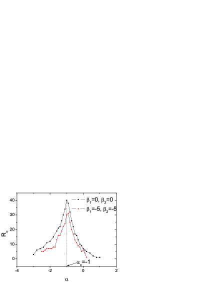
Figure 1: (color online) The network capacity $R_{c}$ against $\alpha$ in cases 1 and 2.

Fig.2 compares the network capacity $R_{c}$ in case 1 and in case 3 (where $\beta_{1}=-2.0$ and $\beta_{2}=2.0$) and case 4 (where $\beta_{1}=-5.0$ and $\beta_{2}=5.0$), i.e., most packets travel from low-degree nodes to high-degree nodes. One can see that the network capacity is greatly enhanced in cases 3 and 4. The maximum network capacity increases from 40 in case 1 to 119 in case 3 and to 720 in case 4. This is because a high-degree node has much more links and therefore much easier to be found by packets than a low-degree node. Based on this result, we suggest that the local routing strategy is very suitable if the packets are more likely to go from low-degree nodes to high-degree nodes.

Moreover, the optimal value of $\alpha_{c}$ corresponding to the maximum capacity increases from $-1.0$ in case 1 to $-0.9$ in case 3 and to $-0.8$ in case 4. This is also explained from Eq.(3). In case 1, $\alpha_{c}>-1$ means high-degree nodes have more packets. In cases 3 and 4, we have $n_{\mbox{generate}}>0,n_{\mbox{remove}}\approx 0$ for low-degree nodes and $n_{\mbox{generate}}\approx 0,n_{\mbox{remove}}>0$ for high-degree nodes. The packets generated in low-degree nodes and removed in high-degree nodes enable the average number of packets on nodes to be independent of degree $k$. As a result, the maximum capacity is achieved.

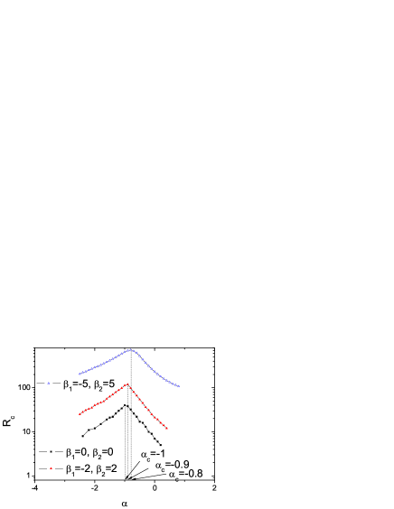
Figure 2: (color online) The network capacity $R_{c}$ against $\alpha$ in cases 1, 3 and 4.

Fig.3 compares the network capacity $R_{c}$ in case 1 and in case 5, where $\beta_{1}=5.0$ and $\beta_{2}=-5.0$, i.e., most packets travel from high-degree nodes to low-degree nodes. One can see that the network capacity becomes smaller and the optimal value of $\alpha_{c}$ decreases. The reason of capacity decrease is the same as in case 2, i.e., a low-degree node has less links and therefore more difficult to be found by packets. The decrease of $\alpha_{c}$ is explained as follows. In case 1, $\alpha_{c}<-1$ means high-degree nodes have less packets. In case 5, we have $n_{\mbox{generate}}>0,n_{\mbox{remove}}\approx 0$ for high-degree nodes and $n_{\mbox{generate}}\approx 0,n_{\mbox{remove}}>0$ for low-degree nodes. The packets generated in high-degree nodes and removed in low-degree nodes enable the average number of packets on nodes to be independent of degree $k$. Consequently, the maximum capacity is reached at $\alpha_{c}<-1$.

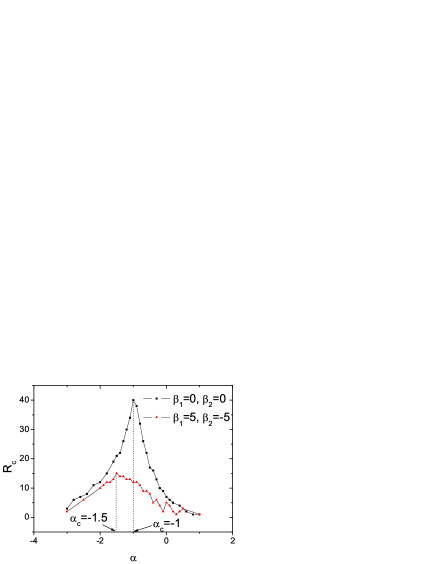
Figure 3: (color online) The network capacity $R_{c}$ against $\alpha$ in cases 1 and 5.

Fig.4 compares the network capacity $R_{c}$ in case 1 and in case 6 (where $\beta_{1}=3.0$ and $\beta_{2}=3.0$) and case 7 (where $\beta_{1}=5.0$ and $\beta_{2}=5.0$), i.e., most packets travel from high-degree nodes to high-degree nodes. In case 6, the network capacity is essentially independent of $\alpha$ for $\alpha<-1$ and decreases with the increase of $\alpha$. In case 7, the network capacity is essentially independent of $\alpha$ when $\alpha$ is in the range studied. This is explained as follows.

In case 6, the probability that the highest-degree node is chosen as origin is 0.33 and it is 0.6 in case 7. Therefore, in case 6, when $R_{c}>31$, the number of particles generated in the highest-degree node exceeds the capacity of the node. This leads to the congestion. As a result, the constant network capacity for $\alpha<-1$ occurs. Similarly, in case 7, when $R_{c}>17$, the number of particles generated in the node exceeds the capacity of the node. Therefore, the constant network capacity in the studied range emerges. To avoid the constant small network capacity, it is necessary to enhance the capacity of the nodes of high degrees.

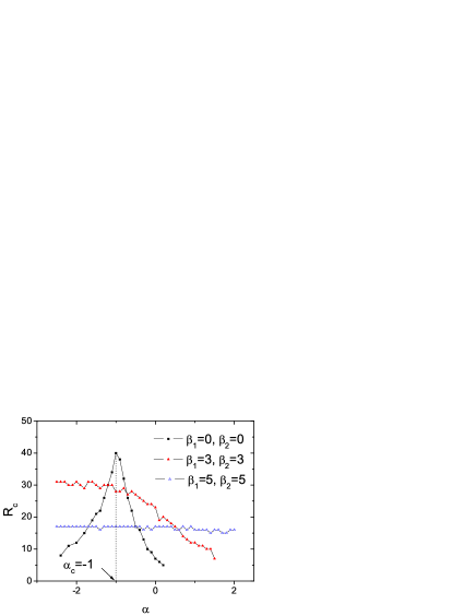
Figure 4: (color online) The network capacity $R_{c}$ against $\alpha$ in cases 1, 6 and 7.

IV Discussion and conclusion

In this paper, we have investigated the network capacity in the scale-free networks, in which packets are generated with non-homogeneously selected sources and destinations, based on the local routing strategy.

Generally speaking, when most packets travel to low-degree nodes, the network capacity will decrease. In contrast, when most packets travel to high-degree nodes, whether the network capacity decreases or increases depends on the selection of origins. When $\beta_{2}$ is large, i.e., most packets are generated from high-degree nodes, the highest-degree node is easily congested, which leads to the congestion of the whole network. To avoid this, it is necessary to enhance the capacity of high-degree nodes. When most packets are generated from low-degree nodes, the network is greatly enhanced. Therefore, the local routing strategy is very suitable if the packets are more likely to go from low-degree nodes to high-degree nodes.

In addition, $\alpha_{c}$, i.e., the optimal value of $\alpha$ corresponding to the maximum network capacity also depends on the distribution of packets’ origins and destinations. We have explained the reason why $\alpha_{c}$ changes when the distribution of packets’ origins and destinations changes.

Finally, we would like to mention that our results may be used to design a new local routing strategy, in which the parameter $\alpha$ is packet-related. Concretely, $\alpha$ depends on the origin and destination of the packet $\alpha=\alpha(k_{o},k_{d})$, where $k_{o}$ and $k_{d}$ denote the degree of the node where the packet is generated and that of the node where the packet goes to. A suitable choice of $\alpha(k_{o},k_{d})$ may enhance the network capacity. Further investigations will be carried out in future work.

References

- (1) R. Albert and A.-L. Barabási, Rev. Mod. Phys. 74, 47 (2002).
- (2) S.N. Dorogovtsev and J. F. F. Mendes, Adv. Phys. 51, 1079 (2002).
- (3) M. E. J. Newman, SIAM Rev. 45, 167 (2003).
- (4) D. J. Watts and S. H. Strogatz, Nature 393, 440 (1998).
- (5) A.-L. Barabási and R. Albert, Science 286, 509 (1999).
- (6) J. D. Noh and H. Rieger, Phys. Rev. Lett. 92, 118701 (2004).
- (7) L. Zhao, K. Park, and Y. C. Lai, Phys. Rev. E 70, 035101(R) (2004).
- (8) G. Yan, T. Zhou, B. Hu, Z.-Q. Fu, and B.-H. Wang, Phys. Rev. E 73, 046108 (2006).
- (9) B. Tadić, S. Thurner, and G. J. Rodgers, Phys. Rev. E 69, 036102 (2004).
- (10) W. X. Wang et al., Phys. Rev. E 73, 026111 (2006).
- (11) W. X. Wang et al., Phys. Rev. E 74, 016101 (2006).
- (12) Z. Y. Chen and X. F. Wang, Phys. Rev. E 73, 036107 (2006).
- (13) A. Arenas, A. Díaz-Guilera, and R. Guimerà, Phys. Rev. Lett. 86, 3196 (2001).