Cascaded generation of multiply charged optical vortices and spatiotemporal helical beams in a Raman medium

Abstract

Using an example of a Raman active medium we describe how a common nonlinear process of four-wave mixing can be used to induce strong coupling between the spatial and temporal degrees of freedom in optical waves. This coupling produces several unexpected effects. Amongst those are cascaded excitation of multiply charged optical vortices, spatial focusing in a nonlinearly defocusing medium and generation of helically shaped spatio-temporal optical solitons.

The nonlinearly mediated interaction between frequency harmonics and the associated effect of frequency conversion have laid the foundation of nonlinear optics shen , and have had an important effect in areas such as fluid dynamics and plasma physics fluids , and - most recently - physics of ultracold matter bec . Four-wave mixing is the most common type of nonlinear wave interaction seen in both crystals with inversion symmetry and isotropic media. In the context of nonlinear optics the four-wave mixing process is typically mediated by Kerr and Raman nonlinearities shen .

Nonlinearity can be used not only to control the spectral, and hence the temporal, properties of waves, but also to transform the linear shen and orbital angular momenta of waves dhol ; des ; dima ; malomed ; raman . In particular, experiments with the second harmonic generation by optical vortices des have demonstrated that two photons with frequency $\omega$ and an orbital angular momentum (OAM) quantum number (or vortex charge) $l$ produce a single photon with frequency $2\omega$ and OAM quantum number $2l$ dhol . Analogous OAM conversion rules have been reported for soliton-like beams within the second harmonic generation model des ; dima , for degenerate four-wave mixing in Kerr-like materials malomed , and for three-wave Raman resonant process with higher order Bessel-beams raman . Though the interplay between spatial and temporal dynamics in nonlinear media has recently become an active research topic, see, e.g. inter , it has failed so far to exploit many of the promising consequences of the strong spatio-temporal coupling seen in frequency conversion experiments using beams with non-zero OAM.

In this work we suggest a method for manipulating the frequency and angular harmonics of light opening new opportunities for simultaneous spatial and temporal shaping of optical waves. We will demonstrate that the exploitation of the coupling between spatial and temporal degrees of freedom can lead to such exciting effects as cascaded vortex generation, strong spatial focusing induced by self-defocusing nonlinearity and the generation of spatio-temporal helical beams in the solitonic and non-solitonic regimes.

One of the most efficient nonlinear optical processes is the Raman mediated four-wave mixing in gases, which easily produces dozens of spectral lines. In particular, it has been demonstrated that the two frequency excitation of a Raman transition away from the resonance can generate, by means of the cascaded four-wave mixing, broad frequency combs and induce nonlinearity related chirp sokolov ; korn ; sokolov1 . The nonlinear chirp can be compensated for by the intrinsic group velocity dispersion (GVD) of the material resulting in the generation of trains of ultra-short (close to single-cycle) pulses sokolov ; korn ; sokolov1 . Note, that the generation of the frequency combs with this technique relies not on the Raman gain, but on a four-wave mixing process which dominates the wings of the Raman line and induces strong effective Kerr nonlinearity prl . The starting idea for the results presented below is that the cascaded off-resonant Raman process, as in sokolov , is initiated under conditions where one of the two (frequency detuned) driving fields is a singly charged vortex beam. In this case, the phase dependent nonlinear coupling between the Raman side-bands (the same coupling, as that which drives frequency conversion) causes cascaded generation of multiply charged vortices. A dimensionless model describing the evolution of the side-bands is sokolov ; ol

$$i\partial_{z}E_{n}-\frac{1}{2}\Delta E_{n}=\beta_{n}E_{n}+q^{*}E_{n-1}+qE_{n+1},$$ (1)

where $n=-N,\dots,0,\dots,N$ and $\Delta=\partial_{x}^{2}+\partial_{y}^{2}$. $E_{n}$ are the dimensionless amplitudes of the sidebands, such that the total field is given by $E_{tot}=\sum_{n}E_{n}(x,y,z)e^{i\Omega_{n}t-iK_{n}z}$, where $\Omega_{n}=(\omega_{0}+n\omega_{mod})/\omega_{mod}$. $\omega_{mod}=\omega_{1}-\omega_{0}$ is the modulation frequency (which is the frequency difference between the two driving fields) and $n=0,1$. The physical frequencies and wavenumbers are represented by the lower case letters $\omega_{n}$ and $k_{n}$, whilst their dimensionless equivalents - by the upper case: $\Omega_{n}$ and $K_{n}$. The dimensionless time $t$ is measured in units of $1/\omega_{mod}$, the propagation coordinate $z$ is in units of $L$, and the transverse coordinates $(x,y)$ are in units of $\sqrt{Lc/\omega_{0}}$. $K_{n}=(\omega_{0}+n\omega_{mod})L/c$ is the scaled free space wavenumber. Here, $L=(\eta\hbar\omega_{0}{\cal N}|b|)^{-1}$ characterizes the coupling length over which power is transferred between neighboring side-bands in the absence of dispersion. $\eta\approx 376$, $\cal N$ is the density of molecules and $b$ is a coefficient characterizing the material dependent coupling between the sidebands sokolov , which weak frequency dependence is neglected for simplicity.

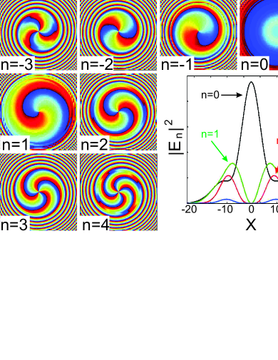
Figure 1: (Color online) The smaller panels show the transverse profiles of the sideband phases ($\arg(E_{n}(x,y))$). The larger panel shows the $x$-distribution of intensities, $|E_{n}(x,y=13)|^{2}$. The propagation distance is $z=0.2$. The window size in each plot is $25\times 25$ dimensionless units (which corresponds to $\simeq 600\times 600\mu m$). The other parameters are: $\mu=5$, $j=-1$, $p_{2}=0.005$, $N=23$. The initial conditions are: $A_{0}=\sqrt{2}$, $A_{1}=1$, $w_{0}=2\sqrt{5}$, $w_{1}=\sqrt{10}$ (see text for more details).

$L$ varies from $1$ to a few mm for $D_{2}$ and $H_{2}$ gases sokolov , so that the one unit of $x$ corresponds to a few tens of microns. $q$, the Raman coherence, is responsible for the coupling between the side-bands. In the adiabatic approximation ol ; pra

$$q={jS\over 2\sqrt{\mu^{2}+|S|^{2}}},\quad S=\sum_{n}E_{n}E_{n+1}^{*},$$ (2)

where $\mu=|\omega_{mod}-\omega_{r}|/(|b|I_{0})$ is the scaled modulus of the detuning of the modulation frequency from the Raman frequency $\omega_{r}$ and $j=sign(\omega_{mod}-\omega_{r})$ is the detuning sign. $|q|$ varies from $0$ to $1/2$ for $|S|$ varying from $0$ to $\infty$. $j=+1$ or $-1$ correspond, respectively, to the self-focusing or self-defocusing nonlinearity induced by the Raman coherence prl ; ol ; pra ; exp . $E_{n}\sqrt{I_{0}}$ are the dimensional amplitudes of the harmonics. For $D_{2}$ and $H_{2}$ gases $\mu=1$ corresponds to $I_{0}\sim 0.1$GW/cm², provided $|\omega_{mod}-\omega_{r}|\sim 1$GHz. The frequency dependence of the propagation constant $\beta(\omega)$ can be fitted with a polynomial, which in the discretized frequency space gives $\beta(\omega_{n})=\beta_{n}=\sum_{i=0}^{M}p_{i}n^{i}$. Without any loss of generality the $p_{0,1}$ coefficients can always be set to zero by phase rotations ol . $p_{2}$ and $p_{i>2}$ characterize GVD and higher order dispersions respectively.

In order to derive the rules for the OAM conversion we assume that the system is pumped with two neighboring sidebands ($n=0,1$) having phases $\phi_{0}$ and $\phi_{1}$, where $\phi_{n}=\Omega_{n}t-(K_{n}-\beta_{n})z+l_{n}\theta$, $\theta=arg(x+iy)$ is the polar angle and $l_{n}$ is the OAM quantum number of the n’s sideband. The conditions for the phase matched excitation of the nearest Stokes and anti-Stokes sidebands are $2\phi_{0}-\phi_{1}=\phi_{-1}$, $2\phi_{1}-\phi_{0}=\phi_{2}$. For an arbitrary $n$ these are generalized as $2\phi_{n}=\phi_{n+1}+\phi_{n-1}$. While the $z$-dependent part of the above condition can not be made zero in dispersive materials ($\beta_{n}\neq 0$), the $t$ and $\theta$ dependent parts are nulled exactly for $\omega_{n}=\omega_{0}+n\omega_{mod}$ and $l_{n}=l_{0}+n(l_{1}-l_{0})$. Therefore, the OAM conversion rule is analogous to the one for the frequencies and $l_{1}-l_{0}$ can be considered as the seeded modulation of OAM. In a particular example considered below $l_{0}=0$ and $l_{1}=1$, so that $l_{n}=n$.

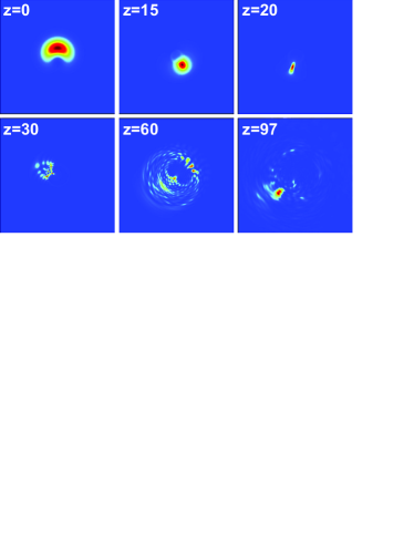
Figure 2: (Color online) Intensity distribution of the total field $|E_{tot}|^{2}$ after different propagation distances $z$ for $t=0$. Azimuthal compression is seen for $z=20$ and subsequent recompression for $z=97$. The nonlinearity is defocusing, $j=-1$. $w_{0}=20\sqrt{5}$, $w_{1}=10\sqrt{10}$. The other parameters are the same as in Fig. 1. The window size is $250\times 250$ dimensionless units.

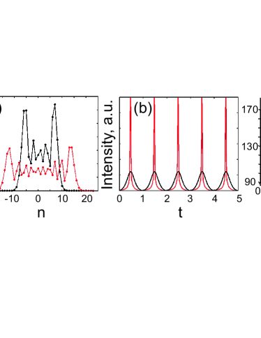
Figure 3: (Color online) Spectral (a) and temporal (b) profiles of the total field $z=10$ (black lines) and $z=20$ (red lines). To plot (a,b) we used the cut through the helix taken at the point of maximal intensity $|E_{tot}|^{2}$. Other parameters are the same as in Fig. 2. (c) Isointensity $(x,y,t)$-plot at $50\%$ of maximum for $z=20$.

For sufficiently strong input fields Raman four-wave mixing should develop in a cascaded manner and excite higher-order Stokes and anti-Stokes fields carrying progressively larger OAM quantum numbers. This process is illustrated in Fig. 1, where we show the transverse profiles of the phases of the side-bands found by numerical integration of Eqs. (1), (2) with 47 sidebands and the initial conditions $E_{0}=A_{0}e^{-r^{2}/w_{0}^{2}}$, $E_{1}=A_{1}re^{i\theta-r^{2}/w_{1}^{2}}$, $E_{n\neq 0,1}=0$ ($r^{2}=x^{2}+y^{2}$). One can see that the generated Stokes ($n<0$) and anti-Stokes ($n>0$) components carry progressively increasing vortex charges, which can be inferred from the number of jumps between the blue (zero phase) and red (phase $2\pi$) colors (see areas around the beam centers in Fig. 1). The efficiency of the OAM conversion (in terms of the phase matching requirements) is the same as the efficiency of the frequency conversion. However, when dealing with spatially inhomogeneous beams one should provide sufficient initial overlap of the two pump fields to build a strong coherence $q$. This is achieved by using a vortex free Gaussian beam wider than the one with a vortex ($w_{0}>w_{1}$).

The above result suggest that the methods of frequency domain wave synthesis sokolov ; korn ; sokolov1 have the potential to be extended to the angular momentum components, and so can be used for simultaneous spatial and temporal beam shaping. This is because, the frequency harmonics in our scheme are, at the same time, the angular harmonics. To start analyzing problem of spatio-temporal beam shaping it is instructive to get some analytical information about the phase evolution under the condition of two field excitation. First, we assume that $E_{n}=f_{n}(r,z)e^{in\theta}$ and that the fields apart from $n=0,1$ are initially zero. Then by neglecting the dispersion ($\beta_{n}=0$) and the $r$-derivatives of $f_{n}$ (i.e., the radial diffraction), we can find an explicit analytical solution to Eqs. (1), (2). This solution gives us $z$-dependence for all $f_{n}$’s in terms of Bessel functions sokolov . Using known identities for the Bessel functions one can find the expression for the total field

$$E_{tot}\simeq e^{i\left[\Omega_{0}t-iK_{0}z+2jz|q_{0}|\cos(t+\theta-Kz+\phi_{0})\right]}$$ (3)

$$\times\left[f_{1}(z=0)+f_{0}(z=0)e^{-i(t-Kz+\theta)}\right],~{}K\equiv L\Omega/c.$$

where $q_{0}=q(z=0)$. In our case, the known result for $E_{tot}$ sokolov is altered by the presence of $\theta$ inside both the phase chirp and amplitude modulation. From the amplitude modulation term one can see that the emerging intensity pattern of $|E_{tot}|$ corresponds to a helix. The helical shape of the isointensity surfaces can be seen in both the $(x,y,t)$ and $(x,y,z)$ subspaces. The time period of the first is $2\pi$ and the spatial period of the second is $2\pi/K$. Changing $l_{1}$ to $-1$ changes the sign in front of $\theta$. One can also note, that the directions of rotation (chirality) of the helices in $t$ and $z$ are opposite.

The phase chirp in (3) is induced by the Raman coherence and plays a crucial role in the evolution of the field, when dispersion and diffraction are taken into account. In typical cases the background dispersion of the gas is normal, meaning that the compensation of the Raman chirp occurs for negative detunings from the Raman resonance ($j=-1$). Since diffraction in general and, in particular, angular diffraction ($\sim\partial_{\theta}^{2}$) is mathematically equivalent to anomalous GVD, it seems at the first glance that the simultaneous temporal and azimuthal compressions for materials with normal GVD are not possible, because the coherence induced azimuthal and temporal chirps have the same sign $j$. The reality, confirmed by numerical modeling, is, however, more intriguing. Indeed, the angular and frequency harmonics in our case have the same complex amplitudes $f_{n}$. This implies that strong coupling between spatial and temporal degrees of freedom occurs in our system. Therefore we can assert that if the characteristic length $L_{com}$, over which maximal pulse compression is achieved, is shorter than the characteristic diffraction length $L_{d}$, then the temporal and azimuthal compression should develop together. Modeling Eqs. (1) with a plane wave excitation and $q_{0}\simeq 0.5$ we found that $L_{com}\simeq 20$ (corresponding to a physical distance of $\sim 2-4$cm), which agrees with Refs. sokolov ; sokolov1 . In our dimensionless notations $L_{d}$ is readily estimated as $L_{d}\sim w_{0,1}^{2}$.

To observe the effect of simultaneous temporal and azimuthal compression with $j=-1$ (defocusing nonlinearity) and normal GVD ($p_{2}>0$) we take the initial excitation like in the modeling shown in Fig. 1, but use wider beams ($w_{0}=10\sqrt{20}$, $w_{1}=10\sqrt{10}$), in order to minimize the role of diffraction over the propagation distances $\sim L_{com}$. The results of this modeling are shown in Figs. 2,3. One can see that for a propagation distance of $z=20$ there are around $30$ harmonics generated, see Fig. 3(a), implying the presence of vortex beams with $|l_{n}|=15$. Simultaneously, a high degree of the temporal and azimuthal compression is achieved, cf. Fig. 2 (z=20) and Fig. 3(b). With further propagation, see Fig. 2, the pulse starts to spread out again producing complicated spatial patterns. However, the compression in this scheme is a quasi-periodic process, and for $z=97$ we observe a clear signature of the second, less pronounced, temporal and azimuthal compression. The spatio-temporal $(x,y,t)$ plot in Fig. 3(c) shows helical structure of the intensity $|E_{tot}|^{2}$ for the propagation distances before strong defragmentation of the transverse profile begins. If we change the detuning sign to $j=1$ (focusing nonlinearity), then the spatiotemporal dynamics is qualitatively different. The compression effect is absent and with the same initial conditions we observed small scale spatial modulational instability and subsequent self-focusing of the emerging filaments developing at $z>30$.

Self-focusing nonlinearity balanced by diffraction suggests the possibility of spatial solitons. Indeed, the latter have been recently reported for the simplest case of a two-component Raman model pra , while Raman self-focusing has been seen experimentally exp . The question, which is relevant for our problem, is whether multi-frequency solitons carrying OAM can be found. To find these structures we assumed that $E_{n}(x,y,z)=f_{n}(r)e^{in\theta+i(\kappa_{1}+n\kappa_{2})z}$, substituted it into Eqs. (1) and solved the nonlinear system of ordinary differential equations for $f_{n}(r)$ numerically. $\kappa_{1,2}$ are the soliton parameters chosen to ensure decay of the soliton tails for $r\to\infty$. The boundary conditions used at $r=0$ are $\lim_{r\to 0}f_{n}r^{-|n|}=const_{n}$. Using this approach we have found a two-parameter ($\kappa_{1},\kappa_{2}$) family of solitons, one example of which is shown in Fig. 4(a). The total intensity corresponding to this solution has a helical profile in both $(x,y,t)$ (not shown, but it is similar to Fig. 3(c)) and $(x,y,z)$ subspaces, see Fig. 4(b). Solitons for sufficiently small values of $\mu$ (implying sufficiently large values of the intensity) are robust with respect to small perturbations, see Fig. 4(b). Taking larger values of $\mu$ leads to excitation of internal oscillations and wobbling helical trajectories, see Fig. 4(c). Notably, experimentally realistic excitation, by just two beams with $l_{0}=0$, $l_{1}=1$, leads to the emergence of structures very close to the found soliton solutions, see Fig. 4(d). This is providing that the input beams are sufficiently narrow, so that the diffraction length is short in comparison to the dispersion length and the self-focusing kicks in before GVD desynchronizes the phases of the harmonics.

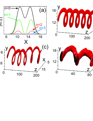
Figure 4: (a) Transverse profiles of $|E_{n}(x,y=13)|^{2}$ for the multi-frequency soliton with $\mu=1$, $j=1$, $p_{2}=0.005$. Soliton parameters are: $\kappa_{1}=-0.5$, $\kappa_{2}=0$. (b) Corresponding evolution of the total intensity $|E_{tot}|^{2}$ along $z$ with $1\%$ noise in the initial conditions. Isointensity plot at $80\%$ of maximum. (c) The same as (b), but for $\mu=5$. (d) Isointensity plot at $20\%$ of maximum for the case of the initial excitation with two beams. $j=1$ and the other parameters as in Fig. 1. In (b),(c) and (d) the total intensity is evaluated for $t=0$.

The helical soliton beams reported here are qualitatively different from the so-called spiralling solitons or rotating soliton clusters spir , which sustain their rotation due to the interaction between the individual beams accompanied by the conservation of the angular momentum. In our case the helical evolution does not require the presence of more than one intensity lobe and originates from the interaction of multiple frequency harmonics carrying progressively growing OAM. Ref. vas studied complex spatial patterns emerging from the linearly interacting vortex beams carrying different OAM, but having identical frequencies. Multicomponent spatial solitons carrying OAM have been reported in segev for a nonlinearity which does not depend on the relative phases of the interacting harmonics, so that the four-wave mixing mediated interaction of the beams has not been included (incoherent interaction). In this case, the OAM of individual components can be arbitrary, i.e. it is not controlled by any selection rules, and higher order vortices can not be generated by the system itself.

In summary: We have demonstrated that a cascaded four-wave mixing process in an off-resonantly excited Raman medium with one of the two input fields being an optical vortex leads to generation of multiply charged optical vortices. Each newly generated vortex beam has its own frequency creating strong dependence between the spatial and temporal degrees of freedom, which can be used for new forms of optical wave synthesis. In particular, we have demonstrated the generation of simultaneous azimuthally and temporally compressed pulses on the defocusing side of the resonance and helical optical solitons on the focusing side. The suggested technique and observed effects pave the way for practical implementations of spatial wave shaping using methods of spectral control. The above concepts are also likely to be applicable for the waves of a different nature.

References

- (1) J.A. Armstrong, N. Bloembergen, J. Ducuing, and P.S. Pershan Phys. Rev. 127, 1918 (1962); Y.R. Shen and N. Bloembergen, Phys. Rev. 137, A1787 (1965).
- (2) N. Bloembergen and Y. R. Shen, Phys. Rev. 141, 298 (1966); T. B. Benjamin and J. E. Feir, J. Fluid Mech. 27, 417 (1967); T. Taniuti and H. Washimi, Phys. Rev. Lett. 21, 209 (1968).
- (3) L. Deng et al., Nature 398, 218 (1999); S. Inouye et al., Science 285, 571 (1999); D. Schneble et al., Science 300, 475 (2003).
- (4) L. Allen, M.J. Padgett, and M. Babiker, Prog. in Optics 39, 291 (1999); A.S. Desyatnikov, Y.S. Kivshar, and L. Torner, Prog. in Optics 47, 291 (2005).
- (5) K. Dholakia et al., Phys. Rev. A 54, R3742 (1996); J. Arlt et al., Phys. Rev. A 59, 3950 (1999); P. Di Trapani et al., Phys. Rev. Lett. 84, 3843 (2000).
- (6) S. Sogomonian, U.T. Schwarz, and H. Maier, J. Opt. Soc. Am B 18, 497 (2001).
- (7) D.V. Skryabin and W.J. Firth, Phys. Rev. E 58, 3916 (1998).
- (8) D. Mihalache et al., Phys. Rev. E 67, 056608 (2003).
- (9) K.S. Syed, G.S. McDonald, G.H.C. New, J. Opt. Soc. Am. B 17, 1366 (2000); D. Salerno et al., Phys. Rev. Lett. 91, 143905 (2003); M. Kolesik, E.M. Wright, and J.V. Moloney, Phys. Rev. Lett. 92, 253901 (2004); A. Vincotte and L. Berge, Phys. Rev. Lett. 95, 193901 (2005).
- (10) A.V. Sokolov and S.E. Harris, J. Opt. B 5, R1 (2003).
- (11) M. Wittmann, A. Nazarkin, and G. Korn, Phys. Rev. Lett. 84, 5508 (2000).
- (12) S. E. Harris and A. V. Sokolov, Phys. Rev. Lett. 81, 2894 (1998); A.V. Sokolov et al., Phys. Rev. Lett. 87, 033402 (2001).
- (13) D.V. Skryabin et al., Phys. Rev. Lett. 93, 143907 (2004).
- (14) A.V. Gorbach and D.V. Skryabin, Opt. Lett. 31, 3309 (2006).
- (15) M.Y. Shverdin, D.D. Yavuz, and D.R. Walker, Phys. Rev. A 69, 031801(R) (2004).
- (16) D.R. Walker et al., Opt. Lett. 27, 2094 (2002).
- (17) L. Poladian, A.W. Snyder, D.J. Mitchell, Opt. Commun. 85, 59 (1991); A.V. Buryak et al., Phys. Rev. Lett. 82, 81 (1999); T. Carmon et al., Phys. Rev. Lett. 87, 143901 (2001); A.S. Desyatnikov and Y.S. Kivshar, Phys. Rev. Lett. 88, 053901 (2002); D.V. Skryabin et al., Phys. Rev. E 66, 055602 (2002).
- (18) M.S. Soskin et al., Phys. Rev. A 56, 4064 (1997); G. Molina-Terriza, J.P. Torres, and L. Torner, Phys. Rev. Lett. 88, 013601 (2002).
- (19) Z.H. Musslimani, M. Segev, D.N. Christodoulides, Opt. Lett. 25, 61 (2000).