Quasistatic limit of the strong-field approximation describing atoms and molecules in intense laser fields

Abstract

The quasistatic limit of the velocity-gauge strong-field approximation describing the ionization rate of atomic or molecular systems exposed to linear polarized laser fields is derived. It is shown that in the low-frequency limit the ionization rate is proportional to the laser frequency, if a Coulombic long-range interaction is present. An expression for the corresponding proportionality coefficient is given. Since neither the saddle-point approximation nor the one of a small kinetic momentum is used in the derivation, the obtained expression represents the exact asymptotic limit. This result is used to propose a Coulomb correction factor. Finally, the applicability of the found asymptotic expression for non-vanishing laser frequencies is investigated.

I Introduction

Keldysh-Faisal-Reiss (KFR) theories are very popular to describe nonresonant multiphoton ionization of atoms and molecules in intense laser fields (see, e. g., Becker et al. (2001); Becker and Faisal (2005); Kjeldsen and Madsen (2006); Milošević et al. (2006) and references therein). While the principle concept of ignoring the effect of the laser field in the initial state and the interaction of the ionized electron with the remaining atomic system in the final state is common to all KFR approximations, the approaches differ in the details of their formulation. Whereas the length gauge was used in the original work of Keldysh Keldysh (1965), the velocity gauge was invoked by Reiss Reiss (1980) and Faisal Faisal (1973). Historically, the velocity-gauge variant of KFR theory is also known as strong-field approximation (SFA) Reiss (1992). Although this terminology is not consequently adopted nowadays, this meaning of SFA is used in the present work that discusses exclusively the velocity-gauge variant of KFR.

A natural test of KFR theories is a comparison of its prediction in the tunneling limit with the corresponding one of quasistatic theories Perelomov et al. (1966); Ammosov et al. (1986). The tunneling limit of the length-gauge version of KFR was considered already by Keldysh for the explicit example of a hydrogen atom. In the derivation he employed, however, two additional approximations: the one of a small kinetic momentum and the saddle-point method (SPM). In his detailed work Reiss (1980) about SFA theory Reiss has also used the SPM to obtain an approximation for the generalized Bessel functions (’asymptotic approximation’) that are required for the calculation of the transition amplitude. As in Keldysh’ work he also adopted an expansion assuming a small kinetic momentum in order to derive the differential ionization rate in the tunneling limit. The algebraically cumbersome form of the in Reiss (1980) derived ’asymptotic approximation’ has motivated the development of a simpler form appropriate for the tunneling regime. This approximation Reiss and Krainov (2003) is again based on the SPM and is referred to as ’tunneling 1 approximation’. It was, however, recently criticized by Bauer Bauer (2005) who has shown numerically that the ’tunneling 1 approximation’ is much worse than the ’asymptotic approximation’ in the case of large kinetic momenta. Since neither Reiss (1980) nor Reiss and Krainov (2003) contain explicit asymptotic expressions in the limit of vanishing laser frequency ($\omega\rightarrow 0$), a systematic study of the quasistatic limit on their basis is almost impossible. Recently, the different versions of KFR were numerically compared with quasi-static theories for the hydrogen atom in Bauer (2006). It was found that SFA significantly underestimates the ionization rate, especially in the limit $\omega\rightarrow 0$ or for very strong fields. Since both limits can be well described with quasistatic theories, a comparison of them with the corresponding limit of SFA can provide an insight into the reasons for such a disagreement. The derivation and analysis of such an asymptotic expression for the SFA ionization rate is the main motivation of this work. As is shown below, the SFA rate does not converge to the tunneling result, if long-range Coulomb interactions are present.

The asymptotic limit of SFA for $\omega\rightarrow 0$ is also very interesting, because it may be used for deriving a Coulomb correction factor by comparing this limiting expression with the one of quasistatic theories. Rescaling the SFA rate (for $\omega\neq 0$) in such a way that it agrees with the quasistatic limit for $\omega\rightarrow 0$ is supposed to correct SFA for the otherwise neglected long-range Coulomb interaction between the ionized electron and the remaining ion. Such a Coulomb correction factor was proposed by Becker and Faisal (see Becker and Faisal (2005) and references therein) and is extensively used in their atomic and molecular SFA calculationsBecker et al. (2001); Becker and Faisal (2005). Note, this correction factor is in fact very large and can amount to almost three orders of magnitude for atomic hydrogen and standard parameters of intense femtosecond lasers. Although it is emphasized in Becker and Faisal (2005) that the low-frequency limit of SFA converges to the tunneling result, this is only shown for the case of short-range interactions. As is demonstrated in the present work, the correct asymptotic limit of SFA in the presence of long-range Coulomb interactions differs from the short-range case even qualitatively, since it is proportional to $\omega$, but $\omega$ independent for short-range potentials. Therefore, the present work also allows to directly derive an asymptotically correct Coulomb correction factor for SFA.

The present paper is organized the following way. After a brief description of the ionization rate within SFA in which the basic formulas and notations are introduced (Sec. II.1), an expression is derived in Sec. II.2 that is numerically very convenient for the calculation of generalized Bessel functions and thus the SFA in the quasistatic limit. In Sec. II.3 an exact asymptotic formula is derived for the generalized Bessel functions in the limit $\omega\rightarrow 0$. In this derivation neither the SPM nor any other approximation beyond the ones inherent to SFA are used and it is demonstrated that the SPM yields wrong results for weakly bound systems or very intense fields. In Sec. II.4 two simplifications are introduced that in contrast to the SPM or small-momentum approximation are universally justified in the limit $\omega\rightarrow 0$. This allows to derive an exact analytical expression of the quasistatic limit of the SFA in the presence of long-range interactions that we name QSFA. In Sec. III the QSFA is discussed for the example of atomic hydrogen. After a derivation of the parameters specific to the considered atomic system in Sec. III.1, the rate obtained in the weak-field limit is discussed and compared to tunneling models in Sec. III.2. Based on this comparison, a Coulomb correction factor is derived for SFA and compared to an earlier proposed one. The range of validity of QSFA for standard laser frequencies is explored in Sec. III.3 where also a correction is proposed that is explicitly given for the 1S state of hydrogenic atoms. The findings of this work are summarized in Sec. IV.

II Theory

II.1 Ionization rate

In the single-active-electron approximation, we consider the direct transition of an electron from the initial bound state $\Psi_{0}$ to a continuum state $\Psi_{{\rm\bf p}}$ due to the linear polarized laser field ${\rm\bf F}(t)={\rm\bf F}\cos\omega t$ with period $T=2\pi/\omega$. The total ionization rate is given in the SFA by

$$W_{\rm SFA} = (2\pi)^{-2}\sum_{N\geq N_{0}}\,p_{N}\left(\frac{p^{2}_{N}}{2}+E_{\rm b}\right)^{2}$$ (1)

$$\times \int\limits d\hat{{\rm\bf p}}\,|L(p_{N}\hat{{\rm\bf p}})|^{2}\,|\tilde{\Psi}_{0}(p_{N},\hat{{\rm\bf p}})|^{2}$$

with $\kappa=\sqrt{2E_{b}}$ where $E_{b}$ is the binding energy of the initial bound state $\Psi_{0}$ with its Fourier transform $\tilde{\Psi}_{0}$. The number of absorbed photons $N$ satisfies $N\geq N_{0}=(E_{\rm b}+U_{p})/\omega$ where $U_{p}=F^{2}/(4\omega^{2})$ is the electron’s quiver (ponderomotive) energy due to the laser field. Finally, $p_{N}=\sqrt{2(N\omega-E_{\rm b}-U_{p})}$ is the momentum in the final state for an $N$ photon transition. The function $L({\rm\bf p})$ is defined as

$$L({\rm\bf p})=\frac{1}{T}\int\limits_{0}^{T}e^{iS_{{\rm\bf p}}(t)}dt$$ (2)

where $S(t)$ is given with the aid of the mechanical momentum of the electron, ${\bm{\pi}}(t)={\rm\bf p}+({\rm\bf F}/\omega)\sin\omega t$, as

$$S_{{\rm\bf p}}(t)=\int\limits_{0}^{t}dt^{\prime}\left[E_{\rm b}+\frac{1}{2}{\bm{\pi}}^{2}(t^{\prime})\right]\quad.$$ (3)

For ${\rm\bf p}=p_{N}\hat{{\rm\bf p}}$ the function $L({\rm\bf p})$ can simply be expressed using the generalized Bessel functions (we use for them Reiss’ definition which differs slightly from the one of Faisal) as

$$L(p_{N}\hat{{\rm\bf p}})=(-i)^{N}e^{\xi i}J_{N}(\xi,-z/2)$$ (4)

where $\xi=p_{N}F(\hat{{\rm\bf p}}\cdot\hat{{\rm\bf F}})/\omega^{2}$ and $z=U_{p}/\omega$. In the high-frequency and low-intensity (so called multiphoton) regime the generalized Bessel functions can be very efficiently calculated using an expansion over products of ordinary Bessel functions,

$$J_{N}(a,b)=\sum_{m=-\infty}^{\infty}J_{N-2m}(a)J_{m}(b)\quad,$$ (5)

where only a few terms are required to yield high accuracy.

Consider now the quasistatic limit defined by $\omega\rightarrow 0$. Introducing the Keldysh parameter $\gamma=\kappa\omega/F$, the (inverse) field parameter $\tau=\kappa^{3}/F$, and the variables

$$q_{N}=p_{N}/\kappa\qquad{\rm and}\qquad\zeta=\hat{{\rm\bf p}}\cdot\hat{{\rm\bf F}},$$ (6)

one finds

$$\xi=\frac{\tau q_{N}\zeta}{\gamma^{2}},\quad z=\frac{\tau}{4\gamma^{3}},\quad N_{0}=\frac{\tau}{4\gamma^{3}}(1+2\gamma^{2}).$$ (7)

The condition $\omega\rightarrow 0$ leads to $\gamma\rightarrow 0$, whereas parameter $\tau$ is $\omega$ independent and thus unaffected. Since the numerical values of $q_{N}$ and $\zeta$ are usually of the order of one, both arguments and the index of the generalized Bessel function in (4) approach to infinity. In this case it is very problematic to use (5) for numerical calculations, since very many terms are required and their amplitudes are much larger than the final result. This can lead to large cancellation errors. In the next subsection we solve this problem by a transformation of the integral (2) to a form that is more convenient for numerical calculations.

II.2 Efficient calculation in the quasistatic limit

A very efficient way for the numerical computation of $L(p_{N}\hat{{\rm\bf p}})$ in the tunneling regime is possible by means of performing the integration through the saddle points. Introduction of the new complex variable $u=\sin\omega t$ allows to rewrite (2) as

$$L=\oint\limits_{C_{\rm c}}{\cal F}(u)du$$ (8)

where

$${\cal F}(u) = \frac{e^{iS(u)}}{2\pi f(u)},$$ (9)

$$S(u) = \frac{\tau}{2\gamma^{3}}\int\limits_{C_{u}}\frac{v^{2}+2\gamma q_{N}\zeta v+\gamma^{2}(1+q^{2}_{N})}{f(v)}dv,$$ (10)

$$f(u) = {\rm Sign}[{\rm Im}(u)]\sqrt{1-u^{2}}.$$ (11)

The closed contour $C_{\rm c}$ in Eq. (8) encloses the branch cut $[-1,1]$ of the functions $f(u)$, $S(u)$, and ${\cal F}(u)$. The path of integration $C_{u}$ in Eq. (11) specifies the path around the branch cut starting at $v=i0^{+}$ and terminating at $v=u$. Since $S(u)$ is a multivalued function, we have selected the branch cut along the negative imaginary axis. Nevertheless, function ${\cal F}(u)$ (as well as $f(u)$ ) is analytical in the whole complex plane except its branch cut $[-1,1]$.

There exist two saddle points $u_{\pm}$ of $S(u)$ in the complex plane $u$ defined by $S^{\prime}(u_{\pm})=0$ and given explicitly by

$$u_{\pm}=\gamma\rho\,(-\chi\pm i)$$ (12)

with

$$\rho=\sqrt{1+q_{N}^{2}(1-\zeta^{2})}\geq 1,\quad\chi=q_{N}\zeta/\rho\leq q_{N}\quad.$$ (13)

We introduce the straight contours $C_{\pm}$ that go through the saddle points $u_{\pm}$ and are given parametrically as

$$u(x,Q_{\pm})=u_{\pm}+xQ_{\pm},\quad-\infty<x<\infty$$ (14)

starting at $x\rightarrow-\infty$. The values of $Q_{\pm}$ are chosen in such a way that the contours $C_{\pm}$ are passing through the steepest descent, i. e. as

$$Q_{\pm}=\sqrt{\frac{2i}{S^{\prime\prime}(u_{\pm})}}$$ (15)

where the argument of $Q_{\pm}$ satisfies $-\pi/4<\arg Q_{\pm}<\pi/4$.

As $|u|\rightarrow\infty$, the function ${\cal F}(u)$ decays exponentially to 0 for $|\arg u|<\pi/4$. This allows to transform the contour integral (8) as

$$L=\oint\limits_{C_{+}}{\cal F}(u)du-\oint\limits_{C_{-}}{\cal F}(u)du=L_{+}-L_{-}$$ (16)

where the integrals $L_{\pm}$ can be calculated using (14) as

$$L_{\pm}=\int\limits_{-\infty}^{\infty}Q_{\pm}{\cal F}(u_{\pm}+Q_{\pm}x)dx\quad.$$ (17)

The transformations above could also be used in the context of SPM, where the integration in (17) is performed in an approximate way using an expansion of $S(u)$ at $u=u_{\pm}$ (see next subsection for more details). However, the expression obtained for $L$ within the SPM is only approximate. Since our intention is to perform an exact calculation of $L$ (within a controllable precision), the integration in (17) is done numerically using Gaussian quadrature. Moreover, it is sufficient to calculate only $L_{+}$. Indeed, using

$$f(u^{*}) = -f^{*}(u),\quad Q^{*}_{\pm}=Q_{\mp},$$ (18)

$$e^{iS(u^{*})} = (-1)^{N}\exp[2\xi i]\left\{e^{iS(u)}\right\}^{*}$$ (19)

one obtains

$$L_{-}=-(-1)^{N}\exp\left[2\xi i\right]L^{*}_{+}\quad.$$ (20)

Substituting (20) into (16) yields

$$L=L_{+}+(-1)^{N}\exp\left[2\xi i\right]L^{*}_{+}\quad.$$ (21)

Introducing the absolute value ${\cal L}$ and the argument $\Omega$ of $L_{+}$ we obtain for the generalized Bessel function

$$J_{N}(\xi,-z/2)=2{\cal L}\cos(\xi-\Omega-N\pi/2)$$ (22)

and

$$|L|^{2}=2{\cal L}^{2}\left[1+\cos(2\xi-2\Omega-N\pi)\right].$$ (23)

We stress that no approximations have been done. The highly oscillatory integral (2) has only been modified to a form that is much more convenient for the numerical calculation of $|L|^{2}$ and will be used in the present work to obtain numerical values of the SFA ionization rate $W_{\rm SFA}$ (1) that serve as a reference for the QSFA derived below.

II.3 Generalized Bessel functions in the quasistatic limit

In order to derive (in Sec. II.4) an analytic expression for the SFA rate in the quasistatic limit, it is required to first find the exact limit of $|L|^{2}$ for $\gamma\rightarrow 0$. It follows from (12) that $u_{+}\rightarrow 0$ in the limit $\gamma\rightarrow 0$. Function $f(u)$ is then nearly 1 in the interval $(0,u_{+})$ and $S(u_{+})$ can be calculated using the Taylor expansion of $f^{-1}(u)$ at $u=0$ for ${\rm Im}(u)>0$,

$$f^{-1}(u)=1+\frac{u^{2}}{2}+\frac{3u^{4}}{8}+\dots$$ (24)

Substitution of (24) into (11) and integration yields

$$iS(u_{+})=-\frac{\tau\rho^{3}}{3}-\frac{\tau\rho^{3}\chi(3+\chi^{2})}{6}\,i+O(\gamma^{2})\;.$$ (25)

Performing the Taylor expansion of $S(u)$ at $u=u_{+}$ gives

$$iS(u_{+}+Q_{+}x)=iS(u_{+})-x^{2}+i\frac{\sqrt{2}}{3\sqrt{\tau\rho^{3}}}x^{3}+O(\gamma^{2})$$ (26)

where

$$Q_{+}=\gamma\sqrt{\frac{2f(u_{+})}{\tau\rho}}=\gamma\sqrt{\frac{2}{\tau\rho}}+O(\gamma^{3})$$ (27)

has been used. Due to the smallness of $Q_{+}$, function $e^{iS(u)}$ decays fastly in the vicinity of $u_{+}$. Since the expansions (26) and (24) are expected to be valid in this region, the integrand of $L_{+}$ can be rewritten as

$$Q_{\pm}{\cal F}(u_{\pm}+Q_{\pm}x)=\gamma\,C\,\exp\left[-x^{2}+i\frac{\sqrt{2}x^{3}}{3\sqrt{\tau\rho^{3}}}\right]+O(\gamma^{3})$$ (28)

where

$$C=\frac{1}{2\pi}\sqrt{\frac{2}{\tau\rho}}\exp\left[-\frac{\tau\rho^{3}}{3}-\frac{\tau\rho^{3}\chi(3+\chi^{2})}{6}\,i\right]\;.$$ (29)

Integration over $x$ yields for the absolute value ${\cal L}$ and the argument $\Omega$ of $L_{+}$

$${\cal L} = \gamma\frac{\rho}{\sqrt{3}\pi}K_{1/3}\left(\frac{\tau\rho^{3}}{3}\right)+O(\gamma^{3})$$ (30)

$$\Omega = -\frac{\tau\rho^{3}\chi(3+\chi^{2})}{6}\,+O(\gamma^{2})$$ (31)

where $K_{\nu}$ is the modified Bessel function of the second kind of order $\nu$. Before using this result for a derivation of the ionization rate in the quasistatic limit, it is instructive to compare it to the predictions of the ’asymptotic approximation’ Reiss (1980) and the ’tunneling 1 approximation’Reiss and Krainov (2003) which both are based on the SPM.

It is important to stress that the term proportional to $x^{3}$ is usually ignored, if the SPM is used. Ignoring this term in (28) and integrating over $x$ would yield instead of (30)

$${\cal L}_{\rm SPM} = \frac{\gamma}{\sqrt{2\pi\tau\rho}}\exp\left[-\frac{\tau\rho^{3}}{3}\right].$$ (32)

Although the limit $\gamma\rightarrow 0$ of the ’asymptotic approximation’ is not easily transparent from the equations given in Reiss (1980), a tedious analysis yields exactly the form given in Eq.(22) where $\Omega$ is specified in Eq.(31) and ${\cal L}$ must be substituted with ${\cal L}_{\rm SPM}$ from (32). On the other hand, to obtain the limit $\gamma\rightarrow 0$ of the ’tunneling 1 approximation’ one should substitute ${\cal L}$ and $\Omega$ in Eq.(22) with

$${\cal L}_{\rm Tun1} = \frac{\gamma}{\sqrt{2\pi\tau\bar{\rho}}}\exp\left[-\frac{\tau\bar{\rho}^{3}}{3}\right]+O(\gamma^{3})$$ (33)

$$\Omega_{\rm Tun1} = -\frac{\tau q_{N}\zeta\bar{\rho}^{2}}{2}+O(\gamma^{2})$$ (34)

where $\bar{\rho}=\sqrt{1+q_{N}^{2}}$.

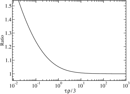
Figure 1: Ratio between ${\cal L}_{\rm SPM}$ (32) and ${\cal L}$ (30) as a function of $\tau\rho^{3}/3$. This ratio indicates the range of validity of the SPM. Since $\rho\geq 1$, the SPM result shows very good agreement for large $\tau$ and starts to fail only for small values of $\tau$. The latter case corresponds to a small binding energy or a high intensity of the field.

Clearly, the ’tunneling 1 approximation’ agrees with the ’asymptotic approximation’ only for $\zeta\approx 0$. It is also evident that for $\zeta\approx 1$ the damping factor in the exponent increases with $q_{N}$, whereas for the ’asymptotic approximation’ it remains at about $-\tau/3$. Since $\zeta\approx 1$ gives the main contribution to ionization, the ’tunneling 1 approximation’ underestimates the ionization rate for larger kinetic momenta as is numerically proven in Bauer (2005).

It is also instructive to check the range of the validity of the SPM used to obtain the ’asymptotic approximation’. The ratio between ${\cal L}_{\rm SPM}$ and ${\cal L}$ is given by

$$\frac{{\cal L}_{\rm SPM}}{{\cal L}}=\frac{\sqrt{\pi}\exp[-\tau\rho^{3}/3]}{\sqrt{2/3}\sqrt{\tau\rho^{3}}K_{1/3}(\tau\rho^{3}/3)}.$$ (35)

Its numerical values for different parameters is shown in Fig. 1. For large values of $\tau\rho^{3}/3$ the ratio is given asymptotically as

$$\frac{{\cal L}_{\rm SPM}}{{\cal L}}\rightarrow 1+\frac{5}{72}\frac{3}{\tau\rho^{3}}=1+\frac{5F}{24\kappa^{3}\rho^{3}}$$ (36)

and approaches 1 in the weak-field limit. For usual laser parameters SPM may give an error within a few percent and only in the extreme case of small binding energies (e. g. ionization of Rydberg states) and very strong fields the error is significantly larger.

II.4 SFA rate in the quasistatic limit

Having obtained an exact asymptotic expression for $|L|^{2}$ it is now possible to derive an analytic form of the SFA ionization rate $W_{\rm SFA}$ (1) in the quasistatic limit. Besides the formulas obtained in the previous two subsections some further asymptotically exact approximations are, however, required. For this purpose, defining the azimuthal angle $\phi$ around axis parallel to ${\rm\bf F}$ and using

$$\int d\hat{{\rm\bf p}}=\int\limits_{-1}^{1}d\zeta\int\limits_{0}^{2\pi}d\phi$$ (37)

we rewrite Eq.(1) as

$$W_{\rm SFA} = \frac{\kappa^{5}}{16\pi^{2}}\int\limits_{-1}^{1}d\zeta\,\sum_{N\geq N_{0}}\,q_{N}\left(1+q_{N}^{2}\right)^{2}|L|^{2}\,\tilde{\Phi}$$ (38)

where

$$\tilde{\Phi}=\int\limits_{0}^{2\pi}d\phi|\tilde{\Psi}_{0}|^{2}.$$ (39)

Note, the argument of the cosine in Eqs.(23) is proportional to $\gamma^{-3}$ and leads to fast oscillations, if $N$ and $\zeta$ are varied. Thus the contribution of this term to the final result is negligibly small and it is possible to substitute $|L|^{2}$ in (38) with $2{\cal L}^{2}$,

$$W^{\rm ap1}_{\rm SFA} = \frac{\kappa^{5}}{8\pi^{2}}\int\limits_{-1}^{1}d\zeta\,\sum_{N\geq N_{0}}\,q_{N}\left(1+q_{N}^{2}\right)^{2}{\cal L}^{2}\tilde{\Phi}\;.$$ (40)

The next step is to substitute the summation over $N$ by an integral. A standard approach consists of a transformation of the sum into an integral over $q_{N}$. This allows to calculate differential rates, but due to the coupling of $q_{N}$ and $\zeta$ in $\rho$ it is impossible to obtain a simple analytical expression without the use of an expansion (e. g. the small kinetic momentum one, $q_{N}\ll 1$). Instead of the use of a double integral with respect to $q_{N}$ and $\zeta$ we rewrite (40) as a double integral with respect to $\rho$ and $\chi$. Transforming the sum into the integral over $\rho$ with

$$\sum_{N\geq N_{0}}\rightarrow\int\limits_{1}^{\infty}d\rho\frac{\rho\tau}{\gamma(1-\zeta^{2})},$$ (41)

and using

$$1+q_{N}^{2}=\rho^{2}(1+\chi^{2}),\quad\int\limits_{-1}^{1}d\zeta\,\frac{q_{N}}{(1-\zeta^{2})}=\int\limits_{-\infty}^{\infty}d\chi\,\rho$$ (42)

one obtains

$$W^{\rm ap2}_{\rm SFA}=\frac{\kappa^{5}\tau}{8\pi^{2}\gamma}\int\limits_{1}^{\infty}d\rho\,\rho^{6}\int\limits_{-\infty}^{\infty}d\chi(1+\chi^{2})^{2}{\cal L}^{2}(\rho,\chi)\tilde{\Phi}(\rho,\chi)\;.$$ (43)

Substitution of (30) into (43) yields an analytical expression for the quasistatic limit of the SFA (denoted QSFA)

$$W_{\rm QSFA}=\omega\,R(\tau,\kappa)$$ (44)

with

$$R(\tau,\kappa) = \int\limits_{1}^{\infty}\frac{8\tau^{2}}{3\pi}B(\rho,\kappa)K^{2}_{1/3}\left(\frac{\tau\rho^{3}}{3}\right)\,d\rho$$ (45)

$$B(\rho,\kappa) = \rho^{8}\left(\frac{\kappa}{4\pi}\right)^{3}\int\limits_{-\infty}^{\infty}d\chi\,(1+\chi^{2})^{2}\,\tilde{\Phi}(\rho,\chi)\;.$$ (46)

If the SPM is used, one has to use (32) instead of (30) in (43). As a consequence, one obtains a similar result, but function $R(\tau,\kappa)$ has to be substituted with

$$R_{\rm SPM}(\tau,\kappa)=\int\limits_{1}^{\infty}\frac{4\tau}{\rho^{3}}B(\rho,\kappa)\exp\left[-\frac{2\tau}{3}\rho^{3}\right]\,d\rho\;.$$ (47)

Eq. (44) is one of the central results of the present work. It shows that the ionization rate calculated within SFA is proportional to the frequency $\omega$ in the limit $\omega\rightarrow 0$. Thus the SFA rate vanishes in the static limit $\omega=0$ for all binding energies and field strengths! Clearly, this prediction of SFA is unphysical implying that SFA is not applicable in the quasistatic limit for atomic systems. As is also clear from the derivation, this conclusion is not a consequence of the usually adopted SPM or small-momentum approximation, since they were not adopted.

The present finding appears to be in conflict with the discussion given, e. g., in Becker and Faisal (2005), where it is explicitly stressed that SFA (corresponding to the first-order S-matrix theory in velocity gauge) approaches the correct tunneling limit for $\omega\rightarrow 0$ (and sufficiently weak fields). However, in Becker and Faisal (2005) (and corresponding references therein) this conclusion is reached on the basis of a derivation valid for short-range potentials, while the present result is obtained for the long ranged Coulomb potential. For short-range potentials the integral over $\chi$ in (46) diverges and one has to consider the term proportional to $\gamma^{2}$ in (25). This term removes the divergence and the obtained limit for the ionization rate is now $\omega$ independent in accordance with the discussion in Becker and Faisal (2005). For long-range potentials there is no divergence in (46), and thus (44) gives the corresponding quasistatic limit of SFA for that case. Clearly, the agreement of the SFA rate with the one predicted by tunneling theories that is obtained for short-range potentials cannot be used as a measure of the validity of the SFA, if long-range potentials are present. However, as is discussed below for the specific example of hydrogen-like atoms, the QSFA results may be used together with tunneling theories to obtain an approximate Coulomb correction factor for SFA.

Since for long-range potentials the SFA rate leads to unphysical results in the quasistatic limit, one would expect that there is very limited interest in its explicit calculation. However, as is shown below, the explicit calculation of $W_{\rm QSFA}$ is not only useful for obtaining a Coulomb correction factor, but it provides also an alternative recipe for an efficient though approximate calculation of SFA rates for atomic and molecular systems exposed to intense laser fields in a large range of experimentally relevant laser parameters. To demonstrate this, calculations for hydrogen-like atoms using Eqs. (44) to (46) are discussed in the next section.

III Quasistatic limit of SFA for hydrogen-like atoms

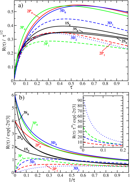
Figure 2: (Color online) The proportionality coefficient $R(\tau)=W_{\rm QSFA}/\omega$ (45) is shown for the complete range of $\tau=(2E_{\rm b})^{3/2}/F$ values for the different hydrogen-like states with $n\leq 3$. a) For small $\tau$ (corresponds to a strong field $F$ or a small binding energy $E_{\rm b}$) all coefficients decrease with decreasing $\tau$. To partly compensate this effect all coefficients $R(\tau)$ are scaled by factor $\sqrt{\tau}$. b) For large $\tau$ (corresponds to a weak field $F$ or a large binding energy $E_{\rm b}$) all coefficients are scaled by the factor $\exp[-2\tau/3]$ (in the insert the coefficients for $m>0$ are also shown scaled by the factor $\tau^{-m}\exp[-2\tau/3]$). In this limit the coefficients $R(\tau)$ tend to those given by (51).

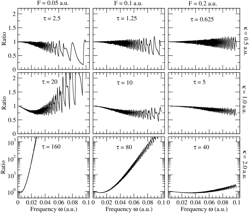
Figure 3: Ratio $W_{\rm SFA}/W_{\rm QSFA}$ for the 1S state of a hydrogenlike atom as a function of the frequency $\omega$ for different field strength $F$ and electron binding energies $E_{\rm b}=\kappa^{2}/2$.

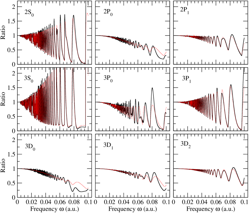
Figure 4: (Color online) The ratios $W_{\rm SFA}/W_{\rm QSFA}$ (black solid) and $W^{\rm ap1}_{\rm SFA}/W_{\rm QSFA}$ (red dotted) are shown as a function of the frequency $\omega$ for all atomic states ($n\leq 3$) and an electron binding parameter $\kappa=0.5\,$a. u. at the field strength $F=0.05\,$a. u. Since both curves are in relatively good agreement with each other, the 1st step in the derivation of the QSFA discussed in Sec.II.4 is valid also for finite values of $\omega$.

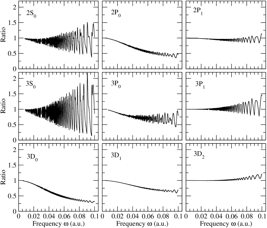
Figure 5: As Fig. 5, but for field strength $F=0.1\,$a.u. and the electron binding parameter $\kappa=1\,$a. u. (Only ratio $W_{\rm SFA}/W_{\rm QSFA}$ is shown.)

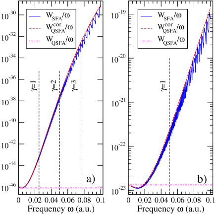
Figure 6: (Color online) The exact SFA rate $W_{\rm SFA}$, the QSFA rate $W_{\rm QSFA}$, and the corrected QSFA rate $W^{\rm cor}_{\rm QSFA}$ (all scaled by $\omega^{-1}$) are shown for the 1S state of a hydrogenlike atom with $\kappa=2\,$a. u. at a) $F=0.05\,$a. u. and b) $F=0.1\,$a. u. The frequencies $\omega$ corresponding to various values of Keldysh parameter $\gamma$ are indicated with dashed lines.

III.1 Proportionality coefficient $R$

In the case of bound states of hydrogen-like atoms the integral over $\chi$ in (46) can be analytically calculated using the identity

$$\int\limits_{-\infty}^{\infty}\frac{d\chi}{(1+\chi^{2})^{n}}=\pi\frac{(2n-3)!!}{(2n-2)!!}.$$ (48)

For example, the Fourier transform of the 1S₀ state is given by

$$\tilde{\Psi}_{0}=\frac{16\pi}{\kappa^{3/2}}\frac{1}{(1+q^{2}_{N})^{2}}\frac{1}{\sqrt{4\pi}}$$ (49)

resulting in

$$\tilde{\Phi}(\rho,\chi)=\frac{2^{7}\pi^{2}}{\kappa^{3}\rho^{8}(1+\chi^{2})^{4}}\;.$$ (50)

Substitution of (50) into (46) and integration over $\chi$ yields $B_{\rm 1S_{0}}=1$. The functions $B(\rho)$ for all hydrogenic states with principal quantum number $n\leq 3$ are listed in Appendix A. Note, for hydrogen-like states the function $B(\rho)$ is $\kappa$-independent and, therefore, the proportionality coefficient $R$ is a function of $\tau$ only. The evaluation of $R$ according to Eq. (45) can then simply be performed numerically. Since the integrand is a smooth exponentially decaying function [this is directly evident, if the SPM approximation is adopted as in (47)], quadrature can easily and very efficiently be performed with high precision.

The proportionality coefficients $R(\tau)$ for a variety of states of hydrogen-like atoms are shown in Fig. 2 for the complete range of values of the inverse field parameter $\tau$. In Fig. 2 a the range $\tau\leq 1$ is shown. For better visibility the function $R(\tau)/\sqrt{\tau}$ is plotted instead of $R(\tau)$. It is worth noticing that for very small $\tau$ the $R$ values for all states approach 0. This is a known failure of SFA, since a larger field intensity to binding energy ratio (and thus smaller $\tau$) should clearly result in a larger and not in a smaller ionization rate Bauer (2006).

In the $\tau$ range shown in Fig. 2 a in which the $R$ values follow the expected behavior (decreasing $R$ for increasing $\tau$), the different states vary rather differently as a function of $\tau$. It is clearly visible that $R$ depends mostly on the quantum numbers $l$ and $m$ and only very weakly on $n$. A different dependence is found for large values of $\tau$ as is discussed below.

III.2 Weak-field limit

The weak-field limit $F\rightarrow 0$ corresponds to $\tau\rightarrow\infty$. Using an asymptotic expansion for the modified Bessel function one finds that the integrand in (45) is proportional to $\exp[-2\tau\rho^{3}/3]$. For large values of $\tau$ the integrand decays thus rapidly as $\rho$ increases. Therefore, it is possible to use an expansion in terms of $\rho$ at $\rho=1$. This procedure yields

$$R_{nlm}(\tau)\rightarrow C^{\rm QSFA}_{nlm}(2\tau)^{-|m|}e^{-2\tau/3}.$$ (51)

The general expression for the coefficients $C^{\rm QSFA}_{nlm}$ is quite complicated. A very simple result occurs, however, for $m=0$ where $C^{\rm QSFA}_{nl0}=2n$ is obtained. Note, in this case the coefficient is $l$-independent. For $n\leq 3$ the coefficients are given by

$$C^{\rm QSFA}_{nlm}=2n\frac{[2n(n-l)+2|m|-1]!!}{[2n(n-l)-1]!!}\;.$$ (52)

Noteworthy, the $l$ dependence is in fact limited to the circularity of the hydrogenic state, since $l$ appears only in the form $n-l$.

In Fig.2 b function $R$ is shown (after multiplying it with $e^{2\tau/3}$ to remove the exponential dependence on $\tau$) as a function of $1/\tau$. The weak-field limit corresponds thus to $1/\tau\rightarrow 0$. As predicted, for $m=0$ the scaled function $R$ approaches $C^{\rm QSFA}_{nl0}=2n$ in this case. Due to the $\tau^{|m|}$ factor appearing in (51) the high $|m|$ states are harder to ionize in the weak-field limit. It is also apparent from Fig.2 b that the characteristic dependence on the quantum numbers in the weak-field limit is reached only for $1/\tau\leq 0.1$ to 0.2. For example, down to $1/\tau\approx 0.15$ the QSFA ionization rates of the 2S₀ and 2P₀ states are almost identical.

It is instructive to compare the quasistatic limit of SFA ionization rate in weak-field limit with the well-known quasistatic Popov-Peremolov-Terent’ev (PPT) formula Perelomov et al. (1966),

$$W_{\rm PPT}=|C_{nl}|^{2}\,f_{lm}\,\sqrt{\frac{3}{2\pi}}\,\kappa^{2}\,(2\tau)^{2n-|m|-3/2}\,e^{-2\tau/3}$$ (53)

where

$$|C_{nl}|^{2}\,=\frac{2^{2n}}{n(n+l)!(n-l-1)!},\quad f_{lm}=\frac{(2l+1)(l+|m|)!}{2^{|m|}|m|!(l-|m|)!}\;.$$

The ionization rates $W_{\rm QSFA}$ and $W_{\rm PPT}$ both include the exponential term $\exp[-2\tau/3]$ and the factor $(2\tau)^{-|m|}$, but differ in the remaining part. Introducing the ratio

$$Q_{\rm PPT}=\frac{W_{\rm PPT}}{W_{\rm QSFA}}=\frac{1}{\omega}\frac{2^{2n-2}|C_{nl}|^{2}\,f_{lm}}{C^{\rm QSFA}_{nlm}}\sqrt{\frac{3}{\pi}}\frac{F^{3/2}}{\kappa^{5/2}}\frac{\kappa^{6n}}{F^{2n}}$$ (54)

it is possible to identify four factors that prevent an agreement between the QSFA and PPT predictions. One is due to the (unphysical) $\omega$ dependence of QSFA. Also the constant factors that depend on the quantum numbers $n$, $l$, and $m$ differ. For example, for fixed $n$ and $m=0$ QSFA predicts the same ionization rate for states with different $l$ whereas the PPT formula predicts an $l$ dependence. Then there is a constant factor ($\sqrt{3/\pi}$) that is, however, very close to 1. Finally, both rates differ in their dependence on field strength and binding energy which is expressed as two factors to stress the $n$ dependence or independence.

Since QSFA is the exact asymptotic limit of SFA, Eq. (54) can be used to derive a Coulomb-corrected SFA rate, $W_{\rm CSFA}=Q_{\rm PPT}\,W_{\rm SFA}$. Clearly, the factor $Q_{\rm PPT}$ derived here explicitly for atomic hydrogen could be applied also to other atomic or molecular systems by performing the evident modifications like the introduction of effective quantum numbers Ammosov et al. (1986), such as $n^{*}$, $l^{*}$, etc. Although the range of validity of $W_{\rm CSFA}$ for $\omega\neq 0$ is not directly evident, in contrast to $W_{\rm SFA}$ it at least reaches the tunneling limit. Already in the past efforts have been made to derive Coulomb-correction factors for KFR theories, but so far the resulting rates did not lead to convincing results (see Becker and Faisal (2005) and references therein). Based on some approximations, A. Becker at al. Becker et al. (2001) have proposed a Coulomb correction factor, $C^{2}$. Using this factor, very good agreement is found between experimental and theoretical SFA ionization yields for a large number of atoms and laser frequencies. The comparison is, however, mostly performed on a qualitative level, since the experiments did not provide absolute yields and thus the theoretical and experimental data were adjusted at one common point. In addition, SFA results for atomic hydrogen (with and without $C^{2}$ factor) are compared to full numerical solutions of the time-dependent Schrödinger equation in Becker et al. (2001) and again good agreement is found (on logarithmic scale).

For atomic hydrogen one has $C^{2}=\kappa^{6n}/F^{2n}$ which corresponds just to the last factor in (54). Clearly, the $C^{2}$-corrected SFA rate does not approach the tunneling limit for $\omega\rightarrow 0$. However, the terms missing in $C^{2}$ yield for $\omega=0.05\,$a. u. and the ground state of a hydrogen atom a factor 0.5 - 1.2 for $F=0.05-0.1\,$a. u. This can explain the reasonable agreement of the $C^{2}$-corrected SFA results with the ones of ab initio calculations reported for such parameters in Becker et al. (2001). However, the deviation increases by a factor 10 for the CO₂ laser frequency or for larger $n$. It may be noted that although Becker et al. (2001) contains also comparisons with experimental data obtained with a CO₂ laser, the present work shows that the found agreement is due to the fact that the comparison is made on a relative scale, as mentioned before. In this case the erroneous $\omega$ dependence of SFA (clearly not corrected by the $C^{2}$ factor) is, for example, not visible.

III.3 Range of validity of QSFA

As follows from the derivation, $W_{\rm QSFA}$ in (44) is the exact asymptotic form of the SFA ionization rate $W_{\rm SFA}$ in the limit $\omega\rightarrow 0$. It is of course interesting to investigate the validity regime of QSFA for non-zero values of $\omega$. In fact, as is shown now, QSFA provides for a wide range of parameters a good approximation to SFA even for laser wavelengths of around 800 nm or less.

Fig. 3 shows the ratio $W_{\rm SFA}/W_{\rm QSFA}$ for the 1S state of a hydrogenlike atom as a function of laser frequency for nine different values of the inverse field parameter $\tau$. The variation of $\tau$ is achieved by using three different values for both the binding-energy related quantity $\kappa$ and the field intensity $F$. The (reference) ionization rate $W_{\rm SFA}$ has been calculated numerically using the scheme described in Sec. II.2. All curves approach unity for $\omega\rightarrow 0$ indicating the correctness of the derivation of QSFA as well as numerical consistency. In the case of the smallest shown value of the inverse field parameter, $\tau=0.625$, one notices that the ratio shows an oscillatory behaviour that is due to channel closings that are not resolved in QSFA. The oscillation amplitude increases with $\omega$, but the ratio remains in between about 0.75 and 1.25 in the full frequency range. Therefore, QSFA is correct to within 25%. If one averages over the oscillations, one finds an even much better quantitative agreement between QSFA and SFA. In view of the fact that the SFA rate is known to overestimate the effect of channel closings and that these pronounced channel closing features mostly disappear when averaging over realistic laser parameters (envelope, focal volume etc.), the QSFA can be said to provide a very accurate approximation for the given parameters. Note, $\omega=0.1\,$a. u. corresponds to a laser wave length of about 450 nm and thus the shown frequency range covers a large range of experimentally relevant lasers.

Increasing $\tau$ by decreasing $F$ (but keeping $\kappa$ fixed) leads to larger oscillation amplitudes while the oscillation period increases. Most importantly, the average value of the ratio drops with increasing $\omega$ below 1. QSFA starts to overestimate the SFA rate. Nevertheless, the oscillation averaged QSFA rate deviates for $\tau=2.5$ at 800 nm from SFA by less than 25 %. Increasing $\tau$ by increasing $\kappa$ (for fixed $F=0.2\,$a. u.) decreases the oscillation amplitude. However, the $\omega$ averaged ratio deviates more from unity than for smaller binding energies. Changing $\kappa$ from 0.5 a. u. (corresponding to a binding energy $E_{b}\approx 3.5\,$eV) to 1.0 a. u. (13.6 eV, hydrogen atom) and 2.0 a. u. (27.2 eV, He⁺) changes the ratio at $\omega\approx 0.1\,$a. u. to about 0.75 and 2.0, respectively. From the representative examples shown in Fig. 3 one can see that these are general trends. A decrease of $F$ (fixed $\kappa$) leads to larger oscillation amplitudes and deviations of the averaged ratio from unity. This limits the applicability of QSFA to a smaller $\omega$ range. An increase of the binding energy (fixed $F$) damps the oscillation, but increases the deviation from unity. Combining both results it is clear that QSFA works best for small binding energies and high field strengths and thus for small values of $\tau$. However, $\tau$ alone is not a sufficient parameter to describe the validity of QSFA, as can be seen from the examples shown for $\tau=2.5$ and 5.0. In this example QSFA works better for the larger value of $\tau$ that is realized by enlarging both $E_{b}$ and $F$.

In Figs. 4 and 5 the validity of the QSFA is investigated for different initial states of hydrogen-like atoms. This includes all possible states with $n\leq 3$. Fig. 4 shows the results for $F=0.05\,$a. u. and $\kappa=0.5\,$a. u. These are the same parameters as the ones used for the 1S state in the upper left corner of Fig. 3. The results in Fig. 5 were on the other hand obtained with $F=0.1\,$a. u. and $\kappa=1.0\,$a. u. and correspond therefore to the ones in the middle of Fig. 3. Again, all ratios approach unity for $\omega\rightarrow 0$ as it should be. Comparing the results for the S states one notices that the oscillation amplitude increases with $n$, but the deviation of the $\omega$-averaged results is very similar. The same trend is visible within the P states (for either $m=0$ or $m=1$). For a given $n$ value the oscillations are most pronounced for $l=0$ and decrease with increasing $l$. In view of the $\omega$-averaged results the range of validity of the QSFA as a function of $\omega$ shows, however, a weaker dependence on $l$, but is in fact decreasing for increasing $l$. For a given $n$ and $l$ combination (2P₀ and 2P₁, 3P₀ and 3P₁, or 3D₀, 3D₁, and 3D₂) the $\omega$-averaged ratios indicate that the range of validity of the QSFA increases with $m$. One may notice the close similarity of the results within the series 1S₀, 2P₁, and 3D₂, 2P₀ and 3D₁, as well as 2S₀ and 3P₁. Finally, as was the case for the 1S state, also Figs. 4 and 5 show that a larger value of $\tau$ decreases the oscillation amplitude and increases the validity regime of the QSFA.

Fig. 4 shows in addition the ratio of $W^{\rm ap1}_{\rm SFA}$ [see Eq.(40)] and $W_{\rm QSFA}$. The overall good agreement with the ratio $W_{\rm SFA}/W_{\rm QSFA}$ indicates $W^{\rm ap1}_{\rm SFA}\approx W_{\rm SFA}$. Clearly, the first step in deriving QSFA is well justified for finite frequencies. Especially, the highly oscillatory behavior of the rate due to channel closings is relatively well reproduced by $W^{\rm ap1}_{\rm SFA}$. The main reason for the deviation between SFA and QSFA is thus due to step 2 of the derivation which smoothes out the highly oscillatory behavior of the rate if $\omega$ is varied.

It is instructive to investigate the main reason for the failure of QSFA to reproduce SFA for large values of $\tau$. It turns out that for large $\tau$ it is most essential to consider in Eq. (25) also the terms proportional to $\gamma^{2}$. This yields (see Appendix B)

$$W^{\rm cor}_{\rm QSFA}=C_{\rm cor}W_{\rm QSFA}$$ (55)

where the correction factor (for a hydrogenlike 1S state) is given by

$$C_{\rm cor}(\gamma)=\frac{\exp\left[-\frac{2\tau}{3}f_{0}(\gamma)\right]}{\left(1+\left[\frac{\pi\tau}{6}f_{2}(\gamma)\right]^{6/7}\right)^{7/12}}\;.$$ (56)

This correction significantly increases the range of validity of the quasistatic formula. Fig. 6 shows a direct comparison of $W_{\rm SFA}$ and $W^{\rm cor}_{\rm QSFA}$ (both scaled by $\omega^{-1}$) for those two case where QSFA failed most severely for the 1S state of a hydrogenlike atom, $\kappa=2.0\,$a. u. and $F=0.05$ or 0.1 a. u. Besides the oscillatory behavior of SFA that is also not reproduced in the corrected QSFA, the overall agreement is very good, even if the rate varies by many orders of magnitude, if $\omega$ changes from 0 to 0.1 a. u. The results of the corrected QSFA are not only interesting for improving the QSFA, but they also confirm once more that the two steps made in the derivation of the QSFA are justified. Finally, it is worth noticing that the range of applicability of Eq.(55) is not restricted to a range of parameters that according to the Keldysh parameter $\gamma$ belongs to the quasistatic regime ($\gamma\ll 1$). Fig. 6 shows that it works even for $\gamma>1$.

IV Conclusion

The SFA (KFR theory in velocity gauge) was studied both analytically and numerically in the quasistatic limit. The derived analytical asymptotic expression (QSFA) shows that in the presence of long-range Coulomb interactions and thus for ionization of neutral or positively charged atoms or molecules the SFA rate is proportional to the laser frequency in this limit. This evidently unphysical result indicates a break-down of the SFA. Furthermore, this result shows that in contrast to the case of short-range potentials the SFA rate does not converge to the tunneling limit for weak fields, if long-range Coulomb interactions are present. The analytical result is supported by a numerical study for which an efficient scheme for the numerical evaluation of the SFA transition amplitude has been developed.

Using different states of hydrogenlike atoms as an example, the predictions of the original SFA and the QSFA are compared to each other. It is found that QSFA allows for a rather accurate prediction of the SFA rate even for finite laser frequencies extending in some favorable cases to wavelengths of 500 nm and below. It is shown that the validity regime of the QSFA can even be extended using a correction factor that is explicitly derived for 1S states. The large range of applicability of the QSFA is of practical interest, since its numerical evaluation is simpler than the one of the original SFA rate, especially in the IR and far-IR frequency regime. Furthermore, it is very convenient for studies of the frequency dependence of the SFA rate, since the QSFA is, besides a simple proportionality factor, $\omega$ independent. Thus the QSFA has to be evaluated for a given system and field strength only once. In turn, the relatively large range of laser frequencies in which QSFA and SFA agree demonstrates that also the SFA rate itself is in a wide range of laser parameters only proportional to $\omega$. An exception is the pronounced $\omega$ dependence due to channel closings that is not reproduced by QSFA.

On the basis of a comparison of the QSFA result with the prediction of the Popov-Peremolov-Terent’ev (PPT) formula a Coulomb correction factor is derived. This factor is compared to a previously proposed one that was supposed to be successfully adopted in a wide range of calculations. It is discussed that part of this success may be due to the fact that the comparisons to experimental data was only possible on a relative scale. In this case a number of important terms missing in the previously proposed Coulomb correction factor is not visible.

The goal of this work has been the derivation of an anlytical expression for the SFA in the quasistatic limit in the presence of long-range Coulomb interactions and a discussion of the resulting QSFA in comparison to SFA. The investigation of the validity of the SFA itself by comparing to the results of full solutions of the time-dependent Schrödinger equation is presently underway and will be discussed elsewhere.

Appendix A Functions $B(\rho)$ for different states.

In this Appendix function $B$ defined by Eq. (46) is given explicitly for all states of hydrogen-like atoms fulfilling $n\leq 3$. (Note, for hydrogenlike atoms function $B$ is independent of $\kappa$.)

$$B_{\rm 1S_{0}}(\rho) = 1$$

$$B_{\rm 2S_{0}}(\rho) = 4-12\rho^{-2}+10\rho^{-4}$$

$$B_{\rm 2P_{0}}(\rho) = 2\rho^{-2}$$

$$B_{\rm 2P_{1}}(\rho) = 5\rho^{-2}-5\rho^{-4}$$

$$B_{\rm 3S_{0}}(\rho) = 9-72\rho^{-2}+220\rho^{-4}-280\rho^{-6}+126\rho^{-8}$$

$$B_{\rm 3P_{0}}(\rho) = 12\rho^{-2}-30\rho^{-4}+21\rho^{-6}$$

$$B_{\rm 3P_{1}}(\rho) = 30\rho^{-2}-135\rho^{-4}+\frac{399}{2}\rho^{-6}-\frac{189}{2}\rho^{-8}$$

$$B_{\rm 3D_{0}}(\rho) = \frac{47}{4}\rho^{-4}-\frac{49}{2}\rho^{-6}+\frac{63}{4}\rho^{-8}$$

$$B_{\rm 3D_{1}}(\rho) = \frac{21}{2}\rho^{-4}-\frac{21}{2}\rho^{-6}$$

$$B_{\rm 3D_{2}}(\rho) = \frac{189}{8}\rho^{-4}-\frac{189}{4}\rho^{-6}+\frac{189}{8}\rho^{-8}$$

Appendix B Correction for large $\tau$.

In this Appendix the corrected QSFA given in Eq. (55) is derived. Introducing $G=\gamma\rho$ and $\bar{v}=v/G$, we rewrite $iS(u_{+})$ in (25) as

$$iS(u_{+})=-\frac{\tau\rho^{3}}{3}f(G,\chi)$$ (57)

where

$$f(G,\chi)=\int\limits_{0}^{-\chi+i}\frac{3}{2i}\frac{(\bar{v}+\chi)^{2}+1}{\sqrt{1-G^{2}\bar{v}^{2}}}\,d\bar{v}\;.$$ (58)

The real part of $f(G,\chi)$ can be given using a Taylor expansion with respect to $\chi$ as

$${\rm Re}f(G,\chi)=1+f_{0}(G)+f_{2}(G)\chi^{2}+\dots$$ (59)

where

$$f_{0}(G) = \frac{3(1+2G^{2})\sinh^{-1}G}{4G^{3}}-\frac{3\sqrt{1+G^{2}}}{4G^{2}}-1$$

$$f_{2}(G) = \frac{3}{2}\left[\frac{\sinh^{-1}G}{G}-\frac{1}{\sqrt{1+G^{2}}}\right]\;.$$

For small values of $G$ these functions can be well approximated by $f_{0}(G)\approx-G^{2}/10$, $f_{2}(G)\approx G^{2}/2$ and for $G<4$ they can be fitted with good accuracy by

$$f_{0}(G) \approx -\frac{11G^{2}(14+3G^{2})}{55(28+15G^{2})+54G^{4}}$$ (60)

$$f_{2}(G) \approx \frac{5G^{2}+G^{3}}{10+9G^{2}}e^{-G/5}\;.$$ (61)

A simple correction factor for the 1S state can now be obtained. Indeed, for this case the main contribution comes from $\rho\approx 1$ and one can multiply $W_{\rm QSFA}$ in Eq. (44) by

$$C_{\rm cor}=\exp[-(2\tau/3)f_{0}(\gamma)]\exp[-(2\tau/3)f_{2}(\gamma)\chi^{2}]$$ (62)

The first term in (62) yields an exponential increase with $\gamma$. The second term introduces a damping for $\chi>\sqrt{d}$ where $d=(2\tau/3)f_{2}(\gamma)$. Using the approximate identity (valid within one percent)

$$\int\limits_{-\infty}^{\infty}\frac{e^{-d\chi^{2}}}{(1+\chi^{2})^{2}}d\chi\approx\frac{\pi}{2}\left[1+\left(\frac{\pi d}{4}\right)^{6/7}\right]^{-7/12}$$ (63)

to carry out the integration over $\chi$ one obtains the final result given in Eqs. (55) and (56).

References

- Becker and Faisal (2005) A. Becker and F. H. M. Faisal, J. Phys. B: At. Mol. Phys. 38, R1 (2005).
- Becker et al. (2001) A. Becker, L. Plaja, P. Moreno, M. Nurhuda, and F. H. M. Faisal, Phys. Rev. A 64, 023408 (2001).
- Kjeldsen and Madsen (2006) T. K. Kjeldsen and L. B. Madsen, Phys. Rev. A 74, 023407 (2006).
- Milošević et al. (2006) D. B. Milošević, G. G. Paulus, D. Bauer, and W. Becker, J. Phys. B: At. Mol. Phys. 39, R203 (2006).
- Keldysh (1965) L. V. Keldysh, Sov. Phys. JETP 20, 1307 (1965).
- Reiss (1980) H. R. Reiss, Phys. Rev. A 22, 1786 (1980).
- Faisal (1973) F. H. M. Faisal, J. Phys. B: At. Mol. Phys. 6, L89 (1973).
- Reiss (1992) H. R. Reiss, Prog. Quant. Electr. 16, 1 (1992).
- Perelomov et al. (1966) A. M. Perelomov, V. S. Popov, and M. V. Terent’ev, Sov. Phys. JETP 23, 924 (1966).
- Ammosov et al. (1986) M. V. Ammosov, N. B. Delone, and V. P. Krainov, Sov. Phys. JETP 64, 1191 (1986).
- Reiss and Krainov (2003) H. R. Reiss and V. P. Krainov, J. Phys. A: Math. Gen. 36, 5575 (2003).
- Bauer (2005) J. Bauer, J. Phys. A: Math. Gen. 38, 521 (2005).
- Bauer (2006) J. Bauer, Phys. Rev. A 73, 023421 (2006).