New approaches to model and study social networks

Abstract

We describe and develop three recent novelties in network research which are particularly useful for studying social systems. The first one concerns the discovery of some basic dynamical laws that enable the emergence of the fundamental features observed in social networks, namely the nontrivial clustering properties, the existence of positive degree correlations and the subdivision into communities. To reproduce all these features we describe a simple model of mobile colliding agents, whose collisions define the connections between the agents which are the nodes in the underlying network, and develop some analytical considerations. The second point addresses the particular feature of clustering and its relationship with global network measures, namely with the distribution of the size of cycles in the network. Since in social bipartite networks it is not possible to measure the clustering from standard procedures, we propose an alternative clustering coefficient that can be used to extract an improved normalized cycle distribution in any network. Finally, the third point addresses dynamical processes occurring on networks, namely when studying the propagation of information in them. In particular, we focus on the particular features of gossip propagation which impose some restrictions in the propagation rules. To this end we introduce a quantity, the spread factor, which measures the average maximal fraction of nearest neighbors which get in contact with the gossip, and find the striking result that there is an optimal non-trivial number of friends for which the spread factor is minimized, decreasing the danger of being gossiped.

1 Introduction

Contrary to what may be perceived at a first glance, social and physical models were brought together several times, during the last four centuries. In fact, not only Maxwell and Boltzmann were inspired by the statistical approaches in social sciences to develop the kinetic theory of gases, but one can even cite the English philosopher Thomas Hobbes, who already in the seventeenth century, using a mechanical approach, tried to explain how people acquaintances and behaviors may contribute to the evolution towards a stable absolute monarchy[1, 2]. More than making a historical perspective if these approaches were successful and correct or not, it is almost unquestionable that, at a certain level, there are social phenomena that could be more deeply understood by using approaches of statistical and physical models. Recently[3, 4, 5], this perspective gained considerable strength from the increased interest on - and in several senses well-succeed - network approach, where one describes complex systems by mapping them on a graph (network) of nodes and links and studies their structure and dynamics with the help of some statistical and topological tools from statistical physics and graph theory[6, 7].

When addressing the specific case of a social system, nodes represent individuals and the connections between them represent social relations and acquaintances of a certain kind. Social networks were studied in different contexts[8, 9, 10, 11, 12, 13, 14], ranging from epidemics spreading and sexual contacts to language evolution and vote elections. However, although they are ubiquitous, social networks differ from most other networks, yielding a still broad spectrum of unanswered questions and improvements to be done when studying their statistical and topological properties. In this paper, we will address three fundamental open questions related to the typical structure and dynamics associated to social networks.

The first open question has to do with the modeling of social networks. The recent broad study of empirical social networks has shown that they have three fundamental features common to all of them[15]. First, they present the small-world effect[16] with small average path lengths between nodes and high clustering coefficients meaning that neighbors tend to be connected with each other. Second, they have positive correlations: the highly (poorly) connected nodes tend to connected to other highly (poorly) connected nodes. Third and last, invariably one observes an organization of the network into some subsets of nodes (communities) more densely connected between each other. Although there are arguments pointing out that all these features could be consequence from one another[15], the modeling of specific social networks reproducing quantitatively all these features has not been successful. Using a recent approach to construct networks, based on a system of mobile agents, it is possible to reproduce all these features. In Section 2 we will further show that the degree distributions characterizing social networks typically follow a specific one-parameter distribution, so-called Brody distribution.

The second question is related to the intrinsic nature of the nodes. For certain social networks there are intrinsic features of the individuals which must be considered in the analysis. For instance, the gender in networks of sexual contacts[14] or the hierarchical position in a network of social contacts inside some enterprise. From the network point of view this distinction means to introduce multipartivity in the network, biasing the preferential attachment between nodes that tend to connect with nodes of a certain type. When there are two types of nodes, e.g. men and women, and the connections between them is strongly related to this type, e.g. men can only match women and vice-versa, the standard measures to analyze network structure fails. In particular, the standard clustering coefficient[16], is unable to quantify the connectedness of broader neighborhoods that typically appear in multipartite networks. In Sec. 3 we will revisit some of the clustering coefficients used to study clustering in bipartite networks, and show how the combination of both clustering coefficients can yield good estimates of normalized cycle distributions. Moreover, we will discuss a general theoretical picture of a global measure of increasing order of clustering coefficients according to some suitable expansion.

The third open question has to do with the heterogeneity of nodes in what concerns their influence in the connections and therefore in the propagation phenomena on social networks. In rumor propagation[17], for instance, one usually treats all connections equally in the spread of some signal (opinion, rumor, etc). This is a suitable assumption for situations like the spread of an opinion which is equally interesting to all nodes in the network, for example political opinions to some vote election. However, there are also several social situations where the signal is not equally interesting to all nodes, as the case of spreading of some gossip about some common friend. In these cases there are connections which will be more probably used to spread the signal than others, since not all our friends are also friends of the particular person which is being gossiped about and therefore, either we tend to not tell the gossip to them or they tend to not spread it even if they hear it. In Sec. 4 we will present a simple model for gossip propagation and describe some striking features. Namely, that there is an optimal number of friends, depending on the degree distribution and degree correlations of the entire network, for which the danger to be gossiped is minimized.

Finally, in Sec. 5 we make final conclusions, giving an overview of future questions which could be studied in social networks arising from the topics studied throughout the paper.

2 Modeling social networks: an approach based on mobile agents

Since the study of social networks is mainly concerned with topological and statistical features of people’s acquaintances[8, 9], the modeling of such networks has been done within the framework of graph theory using suitable probabilistic laws for the distribution of connections between individuals[3, 4, 5, 7]. This approach proved to be successful in several contexts, for instance to describe community formation[18, 19] and their growth[20].

Figure 1: Illustration of the two-dimensional mobile agents system. Initially there are no connections between nodes and nodes move with some initial velocity $v_{0}$ in a randomly chosen direction (arrows). At $t=1$ two nodes, $P_{1}$ and $P_{2}$ collide and a connection between them is introduced (solid line), velocities are updated increasing their magnitude and choosing a new random direction. At $t=2$ two other collisions occur, between nodes $P_{2}$ and $P_{4}$ and between nodes $P_{1}$ and $P_{3}$. In this way a network of nodes and connections between them emerges as a straightforward consequence of their motion (see text).

However, they present two major drawbacks. First, the graph approach may be suited to describe the structure of social contacts and acquaintances, but lacks to give insight into the social dynamical laws underlying it. Second, these models seem to be unable to reproduce all the main features characteristic of social networks, at least at the fundamental level. In this context, it was pointed out that[21, 22, 23] dynamical processes based on local information should be also considered when modeling the network. Our recent proposal to overcome these shortcomings was to construct networks, from a system of mobile agents following a simple motion law[13, 14]. Here, we briefly review this model and further present the analytical expression that fits the obtained degree distributions. In particular we show that the degree distribution typically follows a Brody distribution[24].

2.1 The model

The model is given by a system of particles (agents) that move and collide with each other, forming through those collisions the acquaintances between individuals. Consequently, the network results directly from the time evolution of the system and is parameterized by two single parameters, the density $\rho$ of agents characterizing the system composition and the maximal residence time $T_{\ell}$ controlling its evolution. Each agent $i$ is characterized by its number $k_{i}$ of links and by its age $A_{i}$. When initialized each agent has a randomly chosen age, position and moving direction with velocity $v_{0}$ and one sets $k_{i}=0$. While moving, the individuals follow ballistic trajectories till they collide. As a first approximation we assume that social contacts do not determine which social contact will occur next. Therefore, after collisions, the total momentum should not be conserved, with the two agents choosing completely random new moving directions. Figure 1 sketches consecutive stages of the evolution of such a system of mobile agents.

Assuming that large number of acquaintances tend to favor the occurrence of new contacts, the velocity should increase with degree $k$, namely

$$\vec{v}(k_{i})=(\bar{v}k_{i}^{\alpha}+v_{0})\vec{\omega},$$ (1)

where $\bar{v}=1\hbox{\ m/s}$ is a constant to assure dimensions of velocity, $\vec{\omega}=(\vec{e}_{x}\cos{\theta}+\vec{e}_{y}\sin{\theta})$ with $\theta$ a random angle and $\vec{e_{x}}$ and $\vec{e_{y}}$ are unit vectors. The exponent $\alpha$ in Eq. (1) controls the velocity update after each collision. Here, we consider $\alpha=1$. Further, the removal of agents considered here is simply imposed by some threshold $T_{\ell}$ in the age of the agents: when $A_{i}=T_{\ell}$ agent $i$ leaves the system and a new agent $j$ replaces it with $k_{j}=0$, $v_{j}=v_{0}$ and randomly chosen moving direction. The selected values for $T_{\ell}$ must be of the order of several times the characteristic time $\tau$ between collisions, in order to avoid either premature death of nodes. Too large values of $T_{\ell}$ are also inappropriate since in that case each node may on average collide with all other nodes yielding a fully connected network.

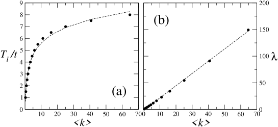
Figure 2: Bridging between real social networks with average degree $\langle k\rangle$ and the system of mobile agents that reproduce their topological and statistical features. In (a) the normalized maximal residence time of agents is plotted as a function of the average degree, while in (b) one plots the collision rate $\lambda$ which is a unique function of the residence time, and scales with $\langle k\rangle$.

Similarly to other systems[25, 26], this finite $T_{\ell}$ enables the entire system to reach a non-trivial quasi-stationary state[13]. In fact, only by tuning $T_{\ell}$ within an acceptable range of small density values, one reproduces networks of social contacts. In Fig. 2a one sees the normalized residence time $T_{\ell}/\tau$ as a strictly monotonic function of the average degree $\langle k\rangle$. From the residence time it is also possible to define a collision rate, as the fraction between the average residence time $T_{\ell}-\langle A(0)\rangle=T_{\ell}/2$ and the characteristic time $\tau$, namely $\lambda=T_{\ell}/(2\tau)=\langle v\rangle T_{\ell}/(2v_{0}\tau_{0})$, where $\tau_{0}$ is the characteristic time of the system at the beginning when all agents have velocity $v_{0}$. Figure 2b shows clearly that $\lambda=2\langle k\rangle$.

By looking at Fig. 2 one now understands the main strength of the mobile agent model here described: when taking a real network of social contacts and measuring the average degree $\langle k\rangle$ the correspondence sketched in Fig. 2 straightforwardly returns the suitable value of $T_{\ell}$ that reproduces the topological and statistical features.

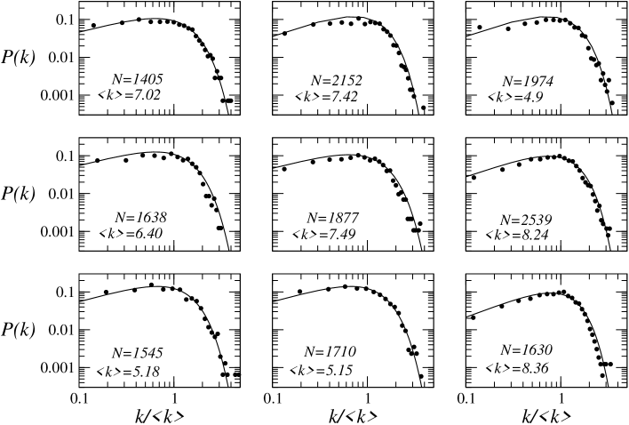
Figure 3: Degree distributions of nine different schools (symbols) from an in-school questionnaire involving a total of $90118$ students which responded to it in a survey between 1994 and 1995. Each school comprehends a number $N$ of interviewed students and from their questionnaires an average number $\langle k\rangle$ of acquaintances is extracted. With solid lines we represent the fit obtained with a Brody distribution, Eq. (2), whose parameter value is computed in Fig. 4.

It was already reported[13, 27] that empirical networks extracted from a survey among $84$ American schools are easily reproduced with this mobile agent model, in what concerns the degree distribution, second-order correlations, community structure, average path length and clustering coefficient. As an illustration, Fig. 3 shows the degree distribution $P(k)$ of nine of such schools (symbols). Such distributions are well fitted by Brody distributions (solid lines) defined as[24]:

$$P_{B}(\bar{k})=\frac{1}{B}(\beta+1)\eta\bar{k}^{\beta}\exp{(-\eta\bar{k}^{\beta+1})},$$ (2)

with $\bar{k}=k/\langle k\rangle$ and

$$\eta=\Gamma\left(\frac{\beta+2}{\beta+1}\right)^{\beta+1}.$$ (3)

and $B$ a normalization constant. Roughly, the Brody distribution in Eq. (2) is, apart some special constants, the product of a power of $k$ with an exponential with a negative exponent proportional to a higher power of $k$. For the particular case $\beta=0$, the Brody distribution reduces to the exponential distribution having always a non-positive derivative.

The distributions in Fig. 3 were obtained with values of $\beta$ slightly above zero, namely between zero and one as shown in Fig. 4. In this case one is able to obtain the non trivial positive slope which is typically observed for small $k$ values in the degree distribution of such social networks. Interestingly, Fig. 4 also shows a linear trend between the average degree $\langle k\rangle$ in the network and the corresponding value of $\beta$ which fits the degree distribution. This guarantees that distribution in Eq. (2) has indeed one single parameter. How such a distribution can be obtained from an analytical approach to the model of mobile agents is still an open question and will be discussed in detail elsewhere.

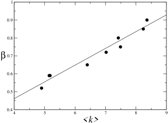
Figure 4: The linear dependence between the parameter $\beta$ of the Brody distribution in Eq. (2) with the average number $\langle k\rangle$ of connections. Each bullet corresponds to one of the schools whose degree distribution is plotted in Fig. 3. The solid line yields the fit $\beta=0.094\langle k\rangle+0.078$.

3 Particular measures for social networks

To measure “the cliquishness of a typical neighborhood” in a network, Watts and Strogatz [16] introduced a simple coefficient, called the clustering coefficient, which counts the number of pairs of neighbors of a certain node which are connected with each other, forming a cycle of size $s=3$. While such tool enables one to access the structure of complex networks arising in many systems [4, 7], helping to characterize small-world networks [16], to understand synchronization in scale-free networks of oscillators [28] and to characterize chemical reactions [29] and networks of social relationships [30, 31], there are other situations where this measure does not suit. Namely, when the network presents a multipartite structure. For instance, when there are two different kinds of nodes and connections link only nodes of different type, the network is bipartite[30, 31, 32] and the bipartite structure does not allow the occurrence of cycles with odd size, in particular with $s=3$.

Bipartite networks are quite common for social systems[32, 33] where the two different kinds of nodes represent e.g. the two genders. While the standard clustering coefficient in such networks is always zero, they have in general non vanishing clustering properties[31] and therefore more appropriate quantities to access such networks have been proposed, namely coefficients counting larger cycles. In this Section, we will discuss how these different clustering coefficients are related to each other and how one can use them to improve the knowledge of the network structure.

The standard clustering coefficient $C_{3}$ is usually defined[16] as the fraction between the number of cycles of size $s=3$ (triangles) observed in the network out of the total number of possible triangles which may appear, namely

$$C_{3}(i)=\frac{2t_{i}}{k_{i}(k_{i}-1)}.$$ (4)

where $t_{i}$ is the number of existing triangles containing node $i$ and $k_{i}$ is the number of neighbors of node $i$, yielding a maximal number $k_{i}(k_{i}-1)/2$ of triangles.

To access the cliquishness in bipartite networks one has proposed[21, 31, 32, 34] a clustering coefficient $C_{4}(i)$, sometimes called the grid coefficient[34], defined as the quotient between the number of cycles of size $s=4$ (squares) and the total number of possible squares. Explicitly, for a given node $i$ with two neighbors, say $m$ and $n$, this coefficient yields[21]

$$C_{4,mn}(i)=\frac{q_{imn}}{(k_{m}-\eta_{imn})(k_{n}-\eta_{imn})+q_{imn}},$$ (5)

where $q_{imn}$ is the number of common neighbors between $m$ and $n$ (not counting $i$) and $\eta_{imn}=1+q_{imn}+\theta_{mn}$ with $\theta_{mn}=1$ if neighbors $m$ and $n$ are connected with each other and $0$ otherwise.

After averaging over the nodes, the coefficients $C_{3}$ and $C_{4}$ characterize the contribution of the first and second neighbors, respectively, for the network cliquishness. In order to be a suitable quantity to measure the cliquishness of bipartite networks compared to their monopartite counterparts, $C_{4}$ must behave the same way as $C_{3}$ when the network parameters are changed, as it is indeed the case for $\langle C_{4}\rangle$ computed from Eq. (5). See Ref. [21] for details.

One should notice that in most $m$-partite networks, it is always possible to have cycles of size $s=4$, indicating that $C_{4}$ is in some sense a more general clustering measure than $C_{3}$. However, it could be the case that for a larger number of partitions forming the network, the contribution of larger cycles increases. This is the case, for instance, of trophic relations in an ecological network of different individuals from different species, where large cycles tend to be abundant, namely the ones ranging from the higher predators to the plants at the lowest trophic level. In such cases, a general clustering coefficient counting the fraction of possible cycles of arbitrary size $n$ may be needed. The generalization is straightforward yielding a clustering coefficient $C_{n}=E_{n}/L_{n}$, where $E_{n}$ is the number of existing cycles with size $n$, $L_{n}$ the maximal number of such cycles that is possible to be attained and $n=3,\dots,N$ for a network of $N$ nodes.

Having $C_{n}$ for the required values of $n$, one is able to introduce a general clustering measure of the network, given by the sum of all these contributions, namely

$$C=\sum_{n=3}^{N}\alpha_{n}C_{n}=\sum_{n=3}^{N}\alpha_{n}\frac{E_{n}}{L_{n}},$$ (6)

where $\alpha_{n}$ is a coefficient that weights the contribution of each different clustering order $n$ and obeys the normalization condition $\sum_{n=3}^{N}\alpha_{n}=1$. In general one can write $E_{n}$ and $L_{n}$ in Eq. (6) as

$$E_{n} = \sum_{k_{1},\dots,k_{n}}NP(k_{1})q(k_{1},k_{2})NP(k_{2})q(k_{2},k_{3})\dots NP(k_{n-1})q(k_{n-1},k_{n})$$ (7)

$$L_{n} = B^{N}_{n}n!=\frac{N!}{(N-n)!}$$ (8)

where $B^{N}_{n}$ are the total combinations of $n$ elements out of $N$, $P(k)$ is the fraction of nodes with $k$ neighbors and $q(k_{1},k_{2})$ is the correlation degree distribution, i.e. the fraction of connections linking a node with $k_{1}$ neighbors to a node with $k_{2}$ neighbors.

From Eq. (7) one can assume approximately that $E_{n}\sim(\langle P\rangle\langle q\rangle N)^{n}$ with $\langle P\rangle$ and $\langle q\rangle$ the average fractions of $P(k)$ and $q(k_{1},k_{2})$ respectively. Since $L_{n}$ increases also as $N^{n}$, a possible suitable choice for $\alpha$ would be a constant, namely $\alpha=1/(N-2)$ obeying the normalization condition above. Having presented this general scenario, we now concentrate on the two first clustering coefficients, $C_{3}$ and $C_{4}$, to address the cycle size distribution.

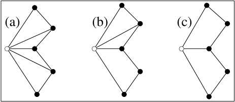
Figure 5: Illustrative examples of cycles (size $s=6$) where the most connected node ($\circ$) is connected to (a) all the other nodes composing the cycle, forming four adjacent triangles. In (b) the most connected node is connected to all other nodes except one, forming two triangles and one sub-cycle of size $s=4$, while in (c) the same cycle $s=6$ encloses two sub-cycles of size $s=4$ and no triangles (see text).

We first show an estimate introduced in Ref. [35], which considers only the degree distribution $P(k)$ and the distribution of the standard clustering coefficient $C_{3}(k)$. One starts by considering the set of cycles with a central node, i.e. cycles with one node connected to all other nodes composing the cycle, as illustrated in Fig. 5a. The central node composes one triangle with each pair of connected neighbors. Due to this fact, the number of cycles with size $s$ can be easily estimated, since the number of different possible cycles to occur is $n_{0}(s,k)=B^{k}_{s-1}\frac{(s-1)!}{2}$, for a central node with $k$ neighbors and the corresponding fraction of these cycles which is expected to occur is $p_{0}(s,k)=C_{3}(k)^{s-2}$, yielding a total number of $s$-cycles given by

$$N_{s} = Ng_{s}\sum_{k=s-1}^{k_{max}}P(k)n_{0}(s,k)p_{0}(s,k),$$ (9)

where $g_{s}$ is a factor which takes into account the number of cycles counted more than once.

The estimate in Eq. (9) is a lower bound for the total number of cycles since it considers only cycles with a central node. Further, this estimate only accounts for cycles up to size $s\leq k_{max}+1$, with $k_{max}$ the maximal degree and is not suited for bipartite networks where $C_{3}(k)=0$ for all $k$. Bipartite networks are typically composed of a set of nodes as those illustrated in Fig. 5c, where no central node exists.

By using additionally the coefficient $C_{4}(k)$ in a similar estimate, one is now able to take into account several cycles without central nodes. One first considers the set of cycles of size $s$ with one node connected to all the others except one, as illustrated in Fig. 5b. Assuming that this node has $k$ neighbors, $s-2$ of them belonging to the cycle one is counting for, one has $n_{1}(s,k)=B^{k}_{s-2}(s-2)!/2$ different possible cycles of size $s$. The corresponding fraction of such cycles which is expected to occur is given by $p_{1}(s,k)=C_{3}(k)^{s-4}C_{4}(k)(1-C_{3}(k))$. Writing an equation similar to Eq. (9), where instead of $n_{0}(s,k)$ and $p_{0}(s,k)$ one has $n_{1}(s,k)$ and $p_{1}(s,k)$ respectively and the sum starts at $s-2$ instead of $s-1$, one has an additional number $N^{\prime}_{s}$ of estimated cycles which is not considered in estimate (9).

To improve the estimate further one repeats the same approach, taking out each time one connection to the initial central node, increasing by one the number of elementary cycles of size $s=4$. Figure 5c illustrates a cycle of size $s=6$ composed by two elementary cycles of size $4$. In general, for cycles composed by $q$ sub-cycles of size $4$ one finds $n_{q}(s,k)=\frac{(s-q-1)!}{2}B^{k}_{s-q-1}$ possible cycles of size $s$ looking from a node with $k$ neighbors and a fraction $p_{q}(s,k)=C_{3}(k)^{s-2q-2}C_{4}(k)^{q}(1-C_{3}(k))^{q}$ of them which are expected to be observed.

Summing up over $k$ and $q$ yields our final expression

$$N_{s}=Ng_{s}\sum_{q=0}^{[s/2]-1}\sum_{k=s-q-1}^{k_{max}}P(k)n_{q}(s,k)p_{q}(s,k).$$ (10)

where $[x]$ denotes the integer part of $x$. In particular, the first term ($q=0$) is the sum in Eq. (9) and the upper limit $[s/2]-1$ of the first sum is obtained by imposing the exponent of $C_{3}(k)$ in $p_{q}(s,k)$ to be non-negative.

The estimate in Eq. (10) not only improves the estimated number computed from Eq. (9), but also enables the estimate of cycles up to a larger maximal size[21], namely up to $s=2k_{max}$ where $k_{max}$ is the maximal number of neighbors in the network.

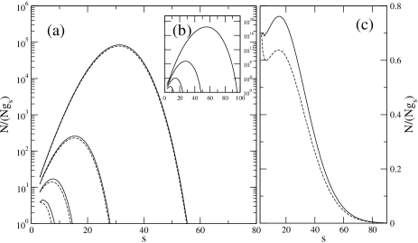
Figure 6: (a) The fraction $N_{s}/Ng_{s}$ of the number of cycles estimated from Eqs. (9), dashed lines, and (10), solid lines, compared with (b) the exact number of cycles as a function of the size for the pseudo-fractal network [36]. From small to large curves one has pseudo-fractal networks with $m=2,3,4,5$ generations (see text). In (c) one sees the comparison between both estimates in a scale-free network with degree distribution $P(k)=P_{0}k^{-\gamma}$ with $P_{0}=0.737$ and $\gamma=2.5$, and coefficient distributions $C_{3,4}(k)=C_{3,4}^{(0)}k^{-\alpha}$ with $C_{3}^{(0)}=2$, $C_{4}^{(0)}=0.33$ and $\alpha=0.9$.

The estimate in Eq. (10) has also the advantage of being able to estimate cycles in bipartite networks. Since for bipartite networks $C_{3}(k)=0$, all terms in Eq. (10) vanish except those for which the exponent of $C_{3}(k)$ is zero, i.e. for $s=2(q+1)$ with $q$ an integer, which naturally shows the absence of cycles of odd size in such networks.

For highly connected networks, both estimates should nevertheless yield similar results, since in that case there is a very large number of both triangles and squares. For instance, the so-called pseudo-fractal network[36] is a deterministic scale-free network, constructed from three initial nodes connected with each other (generation $m=0$), and iteratively adding new generations of nodes such that in generation $m+1$ one new node is added to each edge of generation $m$ and is connected to the two nodes joined by that edge. For these networks, the exact number of cycles with size $s$ can be written iteratively [37] and can be directly compared to the one obtained with the two estimates above. Figure 6a shows the two estimates, while in Fig. 6b the exact number is computed. We notice that both the real number $N_{s}$ of cycles and the normalized value $N_{s}/(Ng_{s})$, though different, yield the same shape. Thus, although the estimates above are not able to explicit the geometrical factor $g_{s}$, the corresponding normalized distributions agree very well with the real one. However, while in this simple situation both estimates are similar, in general they can deviate significantly, as illustrated in Fig. 6c. In such cases, the estimate (10) is closer to the real distribution of cycle sizes[21].

4 Spreading phenomena in social networks

In the previous Section we show how the study of network structure can be addressed by using tools as the clustering coefficient and first and second degree distributions. However, although the ability to communicate within a network of contacts is favored by the network topology[38], to study dynamical phenomena occurring on the network other measures are necessary. Here, we focus on novel properties that help to ascertain the broadness and speed of propagating phenomena through the network. We will describe two helpful quantities to study propagation in a network. As we will see these tools are particularly suited for a simple model of gossip propagation, that yields a striking result: in real social systems it is possible to minimize the risk of being gossiped, by only choosing an optimal number of friendship acquaintances.

We start by introducing the additional quantities in the context of gossip propagation. As opposed to rumors, a gossip always targets the details about the behavior or private life of a specific person. Some information of a specific gossip is created at time $t=0$ about the victim by one of its neighbors. Since typically the gossip tends to be of interest to only those who know the victim personally, we consider first that it only spreads at each time step from the vertices that know the gossip to all vertices that are connected to the victim and do not yet know the gossip. Our dynamics is therefore like a burning algorithm [39], starting at the originator and limited to sites that are neighbors of the victim. The gossip will spread until all reachable neighbors of the victim know it, yielding a spreading time $\tau$.

To measure how effectively the gossip or more generally the amount of information attains the neighbors of the starting node (victim), we define the spreading factor $f$ given by

$$f=n_{f}/k$$ (11)

where $n_{f}$ is the total number of the $k$ neighbors who eventually hear the gossip in a network with $N$ vertices (individuals). Although similar in particular cases, the spreading factor $f$ and the clustering coefficient are, in general, different because the later one only measures the number of bonds between neighbors giving no insight about how they are connected.

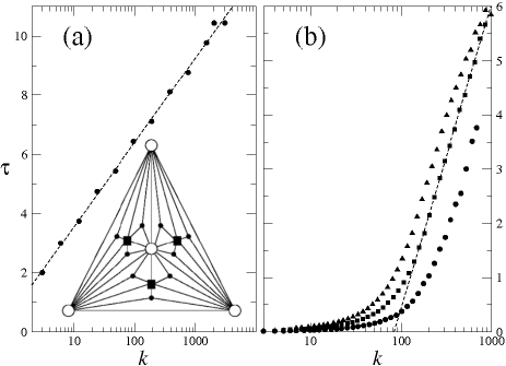
Figure 7: Semi-logarithmic plot of the spreading time $\tau$ as a function of the degree $k$ for (a) the Apollonian ($n=9$ generations) and (b) the Barabási-Albert network with $N=10^{4}$ nodes for $m=3$ (circles), $5$ (squares) and $7$ (triangles), where $m$ is the number of edges of a new site, and averaged over $100$ realizations. In the inset of (a) we show a schematic design of the Apollonian lattice for $n=3$ generations. Fitting Eq. (12) to these data we have $B=1.1$ in (a) and $B=5.6$ for large $k$ in (b).

In Fig. 7 one sees how the spreading time $\tau$ depends on the degree $k$ of the starting node. The Apollonian network[40] is illustrated in Fig. 7a, while the case of Barabási-Albert networks is given in Fig. 7b. In both cases $\tau$ clearly grows logarithmically,

$$\tau=A+B{\rm log}k,$$ (12)

for large $k$. In the case of the Apollonian network, one can even derive this behavior analytically as follows. In order to communicate between two vertices of the $n$-th generation, one needs up to $n$ steps, which leads to $\tau\propto n$. Since for the Apollonian network one has[40] $k=3\times 2^{n-1}$, one immediately obtains that $\tau\propto{\rm log}k$.

For the Apollonian network all neighbors of a given victim are connected in a closed path surrounding the victim, as can be seen from the inset of Fig. 7a, yielding $f=1$. This stresses the fact that the spread factor $f$ is rather different from the clustering coefficient which in this case is $C=0.828$ [40].

Next, we will show that for these two features to appear one needs the existence of degree correlations between connected nodes, as usually observed in real empirical networks. In Fig. 8 we plot the results of gossip spreading on an empirical set of networks extracted from survey data[41] in 84 U.S. schools. Here, the logarithmic growth of $\tau$ with $k$, shown in Fig. 8a, follows the same dependence of the average degree $k_{nn}$ of the nearest neighbors[42], as illustrated in the inset. As in the case of the BA networks, we also find for the schools a characteristic degree $k_{0}$ for which $f$ and therefore the gossip spreading is smallest. The inset of Fig. 8b, however, gives clear evidence that the school networks are not scale-free. Since the same optimal degree appears in Barabási-Albert networks, one argues that the existence of this optimal number is not necessarily related to the degree distribution of the network, but rather to the degree correlations.

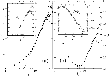
Figure 8: Gossip propagation on a real friendship network of American students [41] averaged over 84 schools. In (a) we show the spreading time $\tau$ and, in the inset, the average degree of neighbors of nodes with degree $k$. In (b) the spread factor $f$, both as a function of degree $k$. In the inset of (b) we see the degree distribution $P(k)$.

However, the relation between degree correlations, measured by $k_{nn}$, and the logarithmic behavior of the spreading time is not straightforward. While in the empirical network we found the same distribution for both $k_{nn}$ and $\tau$, in BA and APL networks $k_{nn}$ follows a power-law with $k$ (not shown). As for the spread factor $f$, a mean field approach can be derived, yielding an $f$-rate equation which depends in general on $P(k)$ and two and three-point correlations of the degree. In the case of uncorrelated networks, two and three-point correlations reduce to simple expressions of the moments of the degree distribution. Therefore, $f$ is independent of the degree, similarly to what is observed for the density of particles as derived by Catanzaro et al[43] in diffusion-annihilation processes on complex networks. For correlated networks, as the empirical network here studied, the analytical approach is not straightforward and will be presented elsewhere.

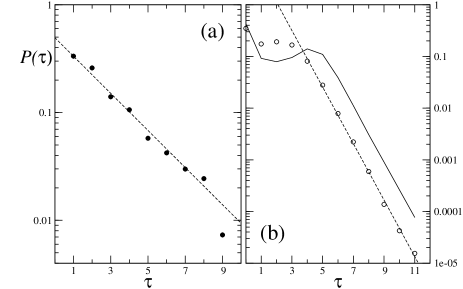
Figure 9: Distribution $P(\tau)$ of spreading times $\tau$ for (a) the APL network of 8 generations, and (b) the real school network (circles) and the BA network with $m=9$ and $N=1000$ (solid line).

Another quantity of interest is the distribution $P(\tau)$ of spreading times, which clearly decays exponentially for the Apollonian network, as illustrated in Fig. 9a. This behavior can be also obtained analytically by considering that $P(\tau)d\tau=P(k)dk$ and using Eq. (12) together with the degree distribution, $P(k)\propto k^{-\gamma}$, to obtain

$$P(\tau)\propto e^{\tau(1-\gamma)/B},$$ (13)

for large $k$. The slope in Fig. 9a is precisely $(1-\gamma)/B=-0.17$ using $B$ from Fig. 7a and $\gamma=2.58$ from Ref. [40]. For the school network, $P(\tau)$ follows also an exponential decay for large $\tau$, but with a 3.5 times smaller characteristic decay time, and has a maximum for small $\tau$, as seen in Fig. 9b (circles). Compared to the $P(\tau)$ of the Barabási-Albert network with $m=9$ (solid line), the shapes are similar but the Barabási-Albert case is slightly shifted to the right, due to the larger minimal number of connections.

Many other regimes of gossip and of propagation phenomena can be also addressed with these two quantities. Namely, a more realistic scenario could be addressed by enabling each node to transfer information with a probability $0\leq p\leq 1$. Further, the assumption that the person to which a gossip did not spread at the first attempt, will never get it, yields a regime similar to percolation conditional to the neighborhood of the victim. Differently, if at each time-step the neighbors which already know the gossip repeatedly try to spread it to the common friends, one observes the same value of $f$ measured for $q=1$, and the spreading time scales as $\tau^{\prime}\sim\tau/q$, where $\tau$ is measured for $q=1$. Finally, other possible regimes comprehend the situation where the gossip spreading over strangers, i.e. over nodes which are not directly connected to the victim. Such cases are being studied in detail and results will be presented elsewhere[44].

5 Discussion and conclusions

In this paper we presented and developed recent achievements in social network research, concerning the modeling of empirical networks, and specific mathematical tools to address their structure and dynamical processes on them.

Concerning the modeling of empirical networks, we described briefly a recent approach based on a system of mobile agents. Further developments were given, namely in what concerns the analytical expression which fits the typical degree distributions observed in empirical social networks. We gave evidence that such distributions follow a Brody distribution which depends on a single parameter that scales with the average degree of the network. A question which now remains to be answered is how to derive such distribution from an analytical and meaningful approach.

Showing that the usual clustering coefficient is, in general, inappropriate when addressing the clustering properties of social networks, we described a suitable measure to access these properties and presented its additional applications for estimating the distribution of cycles of higher order. This additional clustering coefficient was also put in a general framework with different other higher-order coefficients, that could be useful for particular situations of multipartite networks. An expansion combining all possible coefficients was also proposed, motivated by previous works[4], which depends only on the degree distribution and degree-degree correlations. However, computational effort to compute such coefficients increases exponentially with their order and therefore it is not yet clear how useful such an expansion may be.

Finally, to study dynamical processes in social networks, in particular the propagation of information, two simple measures were introduced. Namely, a spread factor, which measures the maximal relative size of the neighborhood reached, when the information starts from a local source (node), and a spreading time, which gives the number of sufficient steps to reach such maximal size. This two measures gave rise to introduce a minimal model for gossip propagation, which can be seen as a particular model of opinions. Within this specific model, the spread factor was found to be minimized by a particular non-trivial degree of the source, which is related to the degree-degree correlations arising in the network. If such possibility of minimizing the danger of being gossiped can be tested in a real situation and which other implications these findings have in other situations - e.g. in internet virus propagation - remain open questions for forthcoming studies.

References

References

- [1] P. Ball, Physica A 314 1-14 (2002).
- [2] P. Ball, Complexus 1 190-206 (2003).
- [3] R. Albert and A.-L. Barabási, Rev. Mod. Phys. 74 47-97 (2002).
- [4] M.E.J. Newman, SIAM Rev. 45 167-256 (2003).
- [5] S.N. Dorogovtsev and J.F.F. Mendes, Adv. Phys. 51 1079-1187 (2002).
- [6] S. Boccaletti, V. Latora, Y. Moreno, M. Chavez and D.-U. Hwanga, Physics Reports 424(4-5), 175-308 (2006).
- [7] B. Bollobás, Modern Graph Theory (Springer, New York, 1998).
- [8] M.E.J. Newman, Proc. Natl. Acad. Sci. 98, 404 (2001).
- [9] M.E.J. Newman, D.J. Watts and S.H. Strogatz, PNAS 99(Supp. 1) 2566-2572 (2002).
- [10] P.L. Krapivsky and S. Redner, Phys. Rev. Lett. 90, 238701 (2003).
- [11] A. Rogers, Phys. Rev. Lett. 90, 158103 (2003).
- [12] L.C. Freeman, The Development of Social Network Analysis (Vancouver, Canada, 2004).
- [13] M.C. González, P.G. Lind and H.J. Herrmann, Phys. Rev. Lett. 96 088702 (2006).
- [14] M.C. González, P.G. Lind and H.J. Herrmann, Eur. Phys. J. B 49, 371-376 (2006).
- [15] M.E.J. Newman and J. Park, Phys. Rev. E 68 036122 (2003).
- [16] D.J. Watts and S.H. Strogatz, Nature 393, 440-442 (1998).
- [17] D.J. Daley and D.G. Kendall, Nature 204, 1118 (1964).
- [18] A. Grönlund, P. Holme, Phys. Rev. E 70 036108 (2004).
- [19] R. Toivonen, J.-P. Onnela, J. Saramäki, J. Hyvönen, K. Kaski, physics/0601114 (2006).
- [20] E.M. Jin, M. Girvan, M.E.J. Newman, Phys. Rev. E 64, 046132 (2001).
- [21] P.G. Lind, M.C. González and H.J. Herrmann, Phys. Rev. E 72, 056127 (2005); cond-mat/0504241.
- [22] J. Davidsen, H. Ebel, and S. Bornholdt, Phys. Rev. Lett. 88, 128701 (2002).
- [23] E. Eisenberg and E.Y. Levanon, Phys. Rev. Lett. 91, 138701 (2003).
- [24] T.A. Brody, Lett. Nuovo Cimento 7 482 (1973).
- [25] L.A.N. Amaral, A. Scala, M. Barthélémy, H.E. Stanley, Proc. Natl. Acad. Sci. 21, 11149 (2000).
- [26] S.N. Dorogovtsev, J.F.F. Mendes, Phys. Rev. E 62, 1842-1845 (2000).
- [27] M.C. González, P.G. Lind and H.J. Herrmann, Physica D 224 137 (2006).
- [28] P.N. McGraw and M. Menzinger, cond-mat/0501663 (2005).
- [29] P.F. Stadler, A. Wagner and D.A. Fell, Adv. Complex Sys. 4, 207-226 (2001).
- [30] M.E.J. Newman, Social Networks 25, 83-95 (2003).
- [31] P. Holme, C.R. Edling and F. Liljeros, Social Networks 26, 155 (2004).
- [32] P. Holme, F. Liljeros, C.R. Edling and B.J. Kim, Phys. Rev. E 68, 056107 (2003).
- [33] R. Guimerà, X. Guardiola, A. Arenas, A. Díaz-Guilera, D. Streib and L.A.N. Amaral, “Quantifying the creation of social capital in a digital community”, private report.
- [34] G. Caldarelli, R. Pastor-Satorras and A. Vespignani, Eur. Phys. J. B 38, 183-186 (2004).
- [35] A. Vázquez, J.G. Oliveira and A.-L. Barabási, Phys. Rev. E 71, 025103(R) (2005).
- [36] S.N. Dorogovtsev, A.V. Goltsev and J.F.F. Mendes, Phys. Rev. E 65, 066122 (2002).
- [37] K. Klemm and P.F. Stadler, Phys. Rev. E 73, 025101(R) (2006); condmat/0506493.
- [38] A. Trusina, M. Rosvall and K. Sneppen, Phys. Rev. Lett. 94, 238701 (2005).
- [39] H.J. Herrmann, D.C. Hong and H.E. Stanley, J.Phys.A 17, L261 (1984).
- [40] J.S. Andrade Jr., H.J. Herrmann, R.F.S. ANDRADE, L.R. da Silva, Phys. Rev. Lett. 94, 018702 (2005).
- [41] Add Health program designed by J.R. Udry, P.S. Bearman and K.M. Harris funded by National Institute of Child and Human Development (PO1-HD31921).
- [42] M. Cantazaro, M. Boguña and R. Pastor-Satorras, Phys. Rev. E 71 027103 (2005).
- [43] M. Cantazaro, M. Boguña and R. Pastor-Satorras, Phys. Rev. E 71, 056104 (2005).
- [44] P.G. Lind, J.S. Andrade Jr., L.R. da Silva, H.J. Herrmann, in preparation (2007).