Spectral transitions in networks

Abstract

We study the level spacing distribution $p(s)$ in the spectrum of random networks. According to our numerical results, the shape of $p(s)$ in the Erdős-Rényi (E-R) random graph is determined by the average degree $\left<k\right>$, and $p(s)$ undergoes a dramatic change when $\left<k\right>$ is varied around the critical point of the percolation transition, $\left<k\right>=1$. When $\left<k\right>>>1$, the $p(s)$ is described by the statistics of the Gaussian Orthogonal Ensemble (GOE), one of the major statistical ensembles in Random Matrix Theory, whereas at $\left<k\right>=1$ it follows the Poisson level spacing distribution. Closely above the critical point, $p(s)$ can be described in terms of an intermediate distribution between Poisson and the GOE, the Brody-distribution. Furthermore, below the critical point $p(s)$ can be given with the help of the regularised Gamma-function. Motivated by these results, we analyse the behaviour of $p(s)$ in real networks such as the Internet, a word association network and a protein protein interaction network as well. When the giant component of these networks is destroyed in a node deletion process simulating the networks subjected to intentional attack, their level spacing distribution undergoes a similar transition to that of the E-R graph.

1 Introduction

A wide class of complex systems occurring from the level of cells to society can be described in terms of networks capturing the intricate web of connections among the units they are made of. Whenever many similar objects in mutual interactions are encountered, these objects can be represented as nodes and the interactions as links between the nodes, defining a network. The world-wide-web, the science citation index, and biochemical reaction pathways in living cells are all good examples of complex systems widely modeled with networks, and the set of further phenomena where the network approach can be used is even more diverse. Graphs corresponding to such real networks exhibit unexpected non-trivial properties, e.g., new kinds of degree distributions, anomalous diameter, spreading phenomena, clustering coefficient, and correlations [1, 2, 3, 4, 5]. In most cases, the overall structure of networks reflect the characteristic properties of the original systems, and enable one to sort seemingly very different systems into a few major classes of stochastic graphs [3, 4]. These developments have greatly advanced the potential to interpret the fundamental common features of such diverse systems as social groups, technological, biological and other networks.

Another general approach to the analysis of complex systems is provided by Random Matrix Theory (RMT), originally proposed by Wigner and Dyson in 1967 for the study of the spectrum of nuclei [6]. Since then, RMT has been successfully used in investigations ranging from the studies of phase transitions in disordered systems [7], through the spectral analysis of chaotic systems [8] and the stock market [9] to the studies of brain responses [10]. Recently, the network approach to complex systems and the RMT were combined in the analysis of the modular structure of biological networks [11]. Network modules, also called as communities, cohesive groups, clusters, etc. correspond to structural sub-units, associated with more highly interconnected parts, with no unique definition [12, 13, 14, 15, 16, 17, 18, 19, 20, 21, 22, 23, 24, 25]. Such building blocks (functionally related proteins [26, 27], industrial sectors [28], groups of people [19, 29], cooperative players [30, 31], etc.) can play a crucial role in forming the structural and functional properties of the involved networks, therefore there has been a quickly growing interest in the last few years in developing efficient methods for locating these modules. One of the most well known community finding algorithm today is the Girvan-Newman algorithm [13, 15], which is based on recursive deletion of links with the highest betweenness. This process leads to splitting of the network to smaller parts, corresponding to the communities, and the deletion of the links is stopped, when optimal modularity is reached.

In the analysis of a protein-protein interaction network and a metabolic network, Luo et al. found that the fluctuations of the level spacing in the spectrum obey different statistics when the networks are split to the communities given by the Girvan-Newman algorithm compared to the original state [11]. (The spectrum of a network is given by the eigenvalues of its adjacency matrix [32, 33, 34]). For both networks, in the original state the fluctuations of the level spacing followed the statistics of the Gaussian Orthogonal Ensemble (GOE), one of the major statistical ensembles in RMT. However, when the networks were split to communities, the fluctuations in the level spacing became Poissonean, which is another important statistics in RMT. Based on this effect, Luo et al. proposed that the monitoring of such changes in the spectral properties can help the identifications of network modules.

Motivated by these very interesting results, here we study the level spacing fluctuations in the spectrum of networks in a more general frame work. Our investigations of the Erd ̋os-Rényi (E-R) random graph, the Internet, a word association graph and a protein-protein interaction graph show that similar spectral transitions occur in these networks as well. However, our results indicate that such transitions in the spectrum are more likely to be connected to the appearance of a giant component than to the ideal partitioning of the network, since e.g. in the E-R graph communities are totally absent. The paper is organised as follows: first we summarise the most important properties of the level spacing distribution in RMT, then describe our results for the spectral transitions in the E-R graph. Finally, we show that similar spectral transitions can be induced in real networks as well, simply by destroying the giant component, without invoking any sophisticated partitioning of the network to communities.

2 The level spacing distribution

The main object of study in RMT is the set of eigenvalues $\{e_{i}\}$ of the random matrix representing the system under investigation. In case of networks, this matrix corresponds to the adjacency matrix, in which the entry $A_{ij}=1$ if the nodes $i$ and $j$ are linked, otherwise $A_{ij}=0$. (For simplicity, let us neglect the possible directionality and weight of the links). One of the most important results of RMT is that complex systems can be sorted into a few universal classes based on the behaviour of the fluctuations in the level spacing between these eigenvalues. The level spacing $S$ between two adjacent eigenvalues is simply $S_{i}=e_{i+1}-e_{i}$, however the distribution of this quantity cannot be universal, as there are systems in which eigenvalues are more dense/sparse on average compared to others. Therefore, instead the the unfolded level spacings are studied, which can be defined as

$$s_{i}=\frac{e_{i+1}-e_{i}}{\left<S\right>_{i}},$$ (1)

where $\left<S\right>_{i}$ denotes the local average of the level spacing in the vicinity of $e_{i}$. The probability distribution of the unfolded level spacings (which from now on we shall call simply as the level spacing distribution) can be described with the probability density $p(s)$ and the corresponding cumulative distribution $P(s)=\int_{0}^{s}p(x)dx$. Due to the unfolding (1), the expectation value of the level spacing is one:

$$\left<s\right>=\int sp(s)ds=1.$$ (2)

The level spacing distribution of systems with strongly correlated eigenvalues follows the statistics of the GOE, defined as an ensemble of random matrices filled with elements drawn from a Gaussian distribution. In this case $p(s)$ and $P(s)$ are given by the Wigner-Dyson distribution [35] as

$$p_{\rm GOE}(s) = \frac{\pi}{2}s\exp\left(-\frac{\pi}{4}s^{2}\right),$$ (3a)

$$P_{\rm GOE}(s) = 1-\exp\left(-\frac{\pi}{4}s^{2}\right).$$ (3b)

Another important universality class is formed by the systems with no correlation between the eigenvalues, following a Poisson level spacing distribution:

$$p_{0}(s) = \exp(-s),$$ (3da)

$$P_{0}(s) = 1-\exp(-s).$$ (3db)

In chaotic systems with weak disorder, intermediate statistics were observed as well, described by the Brody-distribution [36, 37, 38, 39, 40]:

$$p_{\rm B}(s) = C\alpha s^{\alpha-1}\exp\left(-Cs^{\alpha}\right),$$ (3dea)

$$P_{\rm B}(s) = 1-\exp\left(-Cs^{\alpha}\right).$$ (3deb)

where $C$ is a normalising constant ensuring the fulfil of Eq.(2), and the parameter $\alpha$ determines how far the distribution falls from the two limiting cases. (At $\alpha=1$ we recover the Poisson-distribution, whereas $\alpha=2$ corresponds to the statistics of the GOE). In the next section we shall analyse the level spacing distribution of the E-R graph.

3 Spectral transition in the E-R graph

The concept of random graphs was introduced by Erdős and Rényi [41] in the 1950s in a simple model starting with $N$ nodes, and connecting every pair of nodes independently with the same probability $p$. Even though real networks differ from this simple model in many aspects, the E-R uncorrelated random graph remains still of great interest, since such a graph can serve both as a test bed for checking all sorts of new ideas concerning complex networks in general, and as a prototype of random graphs to which all other random graphs can be compared.

Perhaps the most conspicuous early result on the E-R graphs was related to the percolation transition taking place at $p=1/N$. The appearance of a giant component in a network, which is also referred to as the percolating component, results in a dramatic change in the overall topological features of the graph and has been in the centre of interest for other networks as well. The relative size of the largest component compared to the total number of nodes is determined by the average degree $\left<k\right>=pN$, and the critical point of the transition is at $\left<k\right>=1$.

In our studies concerning the level spacing distribution of the E-R graph, we observed a similar phenomenon: the shape of $p(s)$ is determined by $\left<k\right>$, or in other words, the $p(s)$ of E-R graphs with the same average degree follow the same curve. In Fig.1. we demonstrate this effect by plotting the level spacing distribution for E-R graphs of size $N=5000$ (circles), $N=7000$ (squares) and $N=10000$ (triangles), with average degree $\left<k\right>=0.5$ (white symbols), $\left<k\right>=1$ (gray symbols), and $\left<k\right>=1.5$ (black symbols). (For each parameter setting, the spectrum of several different instances of E-R graphs with the given $N$ and $\left<k\right>$ was evaluated numerically, and the resulting level spacing distributions were averaged). Beside the data collapse for the different $N$ parameters, it can be seen that the level spacing distribution undergoes a dramatic change when $\left<k\right>$ is varied around $\left<k\right>=1$. The $p(s)$ at $\left<k\right>=1$, the critical point of the percolation transition (denoted by gray symbols) is exponential, whereas it shows a somewhat more complex forms for both $\left<k\right><1$ and for $\left<k\right>>1$.

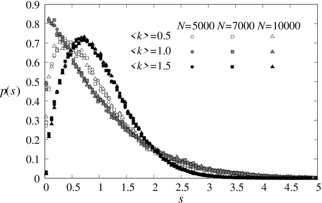
Figure 1: The level spacing distribution $p(s)$ of E-R graphs of size $N=5000$ (circles), $N=7000$ (squares), and $N=10000$ (triangles) at average degree $\left<k\right>=0.5$ (white symbols), $\left<k\right>=1$ (gray symbols), and$\left<k\right>=1.5$ (black symbols). The curves corresponding to different system sizes with the same average coincide with each other.

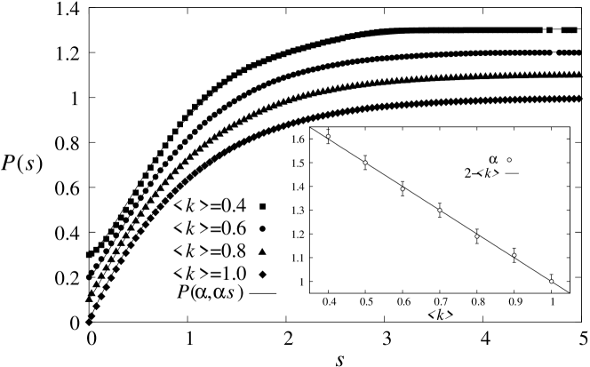
Figure 2: The cumulative level spacing distribution $P(s)$ obtained for $\left<k\right>=0.4$ (squares), $\left<k\right>=0.6$ (circles), $\left<k\right>=0.8$ (triangles), and $\left<k\right>=1$ (diamonds).(The curves corresponding to $\left<k\right><1$ were shifted vertically to give a clearer view). In each case, the empirical $P(s)$ can be very well fitted by $P(\alpha,\alpha s)$ (continuous lines). The inset shows the fitting parameter $\alpha$ as the function of the average degree $\left<k\right>$.

First, let us concentrate on the $\left<k\right><1$ regime. This corresponds to the dispersed state, where the graph consists of small isolated subgraphs. In Fig.2. we plot the observed cumulative level spacing distribution for $\left<k\right>=0.4,0.6,0.8$ and $\left<k\right>=1$. In each case, the empirical results can be very well fitted by

$$p(s) = \frac{\alpha^{\alpha}}{\Gamma(\alpha)}\exp(-\alpha s)s^{\alpha-1}$$ (3defa)

$$P(s) = \frac{\gamma(\alpha,\alpha s)}{\Gamma(\alpha)}=P(\alpha,\alpha s),$$ (3defb)

where $\alpha\in[0,1]$ is the fitting parameter, $\Gamma(\alpha),\Gamma(\alpha,s)$ and $P(\alpha,\alpha s)$ denote the Gamma-function, the incomplete Gamma-function and the regularised Gamma-function respectively, defined as

$$\Gamma(\alpha) = \int_{0}^{\infty}t^{\alpha-1}\exp(-t)dt,$$ (3defga)

$$\gamma(\alpha,s) = \int_{0}^{s}t^{\alpha-1}\exp(-t)dt,$$ (3defgb)

$$P(\alpha,s) = \frac{\gamma(\alpha,s)}{\Gamma(\alpha)}.$$ (3defgc)

The distribution given by (3defb) is normalised, and fulfils (2) as well. The inset in Fig.2. shows the relation between the fitting parameter $\alpha$ and the average degree, which can be expressed simply as

$$\alpha=2-\left<k\right>.$$ (3defgh)

At the critical point of the percolation transition $\alpha$ becomes unity, therefore $P(s)$ given by (3defb) is transformed into $P_{0}(s)=-\exp(s)$, corresponding to Poisson statistics in RMT.

In the $\left<k\right>\geq 1$ regime the graph contains a giant component. Close to the critical point, there are other smaller components present as well, however for large enough $\left<k\right>$ the size of the giant component eventually reaches the system size. The level spacing distribution in the vicinity of $\left<k\right>=1$ can be fitted with the Brody-distribution, given by (3dea-3deb), corresponding to a statistics in between Poisson and GOE. In Fig.3. we demonstrate this effect by plotting $-\log[1-P(s)]$ as the function of $s$ on a logarithmic scale. A cumulative level spacing distribution of the form (3deb) is thereby transformed into $Cs^{\alpha}$, appearing as a straight line with slope $\alpha$. At the critical point of the percolation transition $\alpha=1$, therefore the slope of the corresponding curve (open circles) is unity. The slope of the curves is increasing with the average degree, and at $\left<k\right>=2$ it is already close to $\alpha=2$, corresponding to GOE statistics. In Fig.4. the fitting parameter $\alpha$ is shown as the function of $\left<k\right>$, following a sigmoid curve, reaching the $\alpha=2$ limit closely above $\left<k\right>=2$.

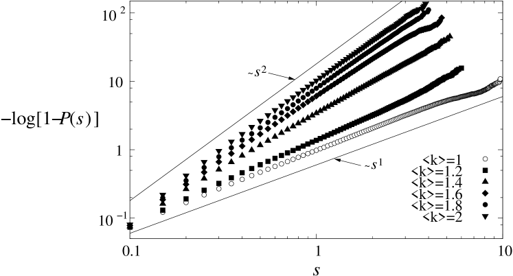
Figure 3: The level spacings of the E-R graph follow the Brody-distribution in the $\left<k\right>\geq 1$ regime. By plotting $-\log[1-P(s)]$ as the function of $s$ on logarithmic scale, the $P_{\rm B}(s)$ given by Eq.(3deb) appears as a straight line with slope $\alpha$. In the limiting case of $\left<k\right>=1$ (open circles) the level spacing distribution is Poissonean with $-\log[1-P(s)]=s$, corresponding to a straight line with unity slope. For $\left<k\right>=1.2$ (squares), $\left<k\right>=1.4$ (triangles up), $\left<k\right>=1.6$ (diamonds), $\left<k\right>=1.8$ (filled circles) and $\left<k\right>=2$ (triangles down) we can observe intermediate level spacing distributions between Poissonean and GOE, shown by straight lines with increasing slopes.

Figure 4: The fitting parameter $\alpha$ in the $\left<k\right>\geq 1$ regime as the function of $\left<k\right>$. Starting from $\alpha=1$ at $\left<k\right>=1$, as the level spacing distribution transforms from Poissonean to GOE, the parameter $\alpha$ reaches $\alpha=2$ following a sigmoid curve.

4 Spectral transition in real networks

Similarly to the E-R graph, spectral transitions can occur in real networks as well. In our studies we examined the behaviour of the level spacing distribution of the Internet, a word association network, and a protein-protein interaction network. In case of the Internet each node corresponded to an Autonomous System, and the links between the Autonomous Systems were obtained from the DIMES project [42]. The word association network was constructed from the South Florida Free Association norms list [43], in which a link from one word to another indicates that people in the surveys associated the end point of the link with its start point. And finally, the studied protein-protein network contained the DIP core list of the protein-protein interactions of S. cerevisiae [44]. These networks are all scale-free, and they consist of 14161, 10617, and 2609 nodes and 43430, 63788, and 6355 links, respectively. In each case, the largest connected component contained more than 90% of the nodes, and the level spacing distribution followed the GOE statistics.

In order to obtain a percolation transition similar to that of the E-R graph, we applied the following recursion to all three networks until their giant components were destroyed:

• calculate the node degrees,

• remove the node with the largest degree.

This algorithm is a variation of the method used to investigate the attack tolerance of networks, where the nodes are removed in the oder of their original degree [45]. Therefore, on one hand, the node removal process above can be also viewed as the simulation of the intentional damage of the investigated networks. On the other hand, the advantage of the present approach compared to the original process in [45] is that we can generate several different configurations of the dispersed state: whenever the largest degree is possessed by more than one node, the algorithm arrives to a branch point with multiple choices for the next node removal.

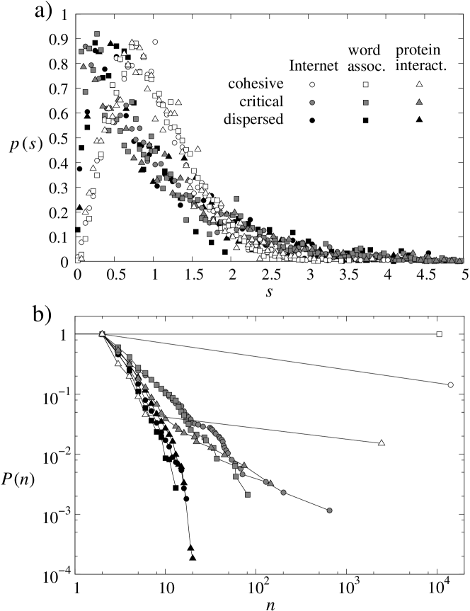
Figure 5: a) The $p(s)$ of the Internet (circles), the word association network (squares) and the protein protein interaction network (triangles) at three stages in the node deletion process: the original cohesive state (white symbols), in the vicinity of the critical point of the percolation transition (gray symbols) and in the dispersed state (black symbols). b) The accompanying cumulative size distributions $P(n)$ with $n$ denoting the number of nodes in the components.

In Fig.5a we plotted the observed level spacing distributions at three stages in the node removal procedure, whereas Fig.5b displays the accompanying cumulative component size distributions $P(n)$, where $n$ denotes the number of nodes in the components. The circles correspond to the Internet, the squares to the word association network, and the triangles to the protein-protein interaction network. The white symbols show the studied distributions in the original cohesive state of the networks: $P(n)$ is dominated by an outstandingly large cluster, the giant component, and $p(s)$ follows GOE statistics. By succedingly removing the nodes with the largest degree, the size of the largest component decreases, and in the vicinity of the critical point of the percolation transition $P(n)$ is transformed into a power-law, and $p(s)$ becomes exponential, as shown by the gray symbols. (These points result from averaging over multiple instances of the critical state, generated by the algorithm detailed above). By continuing the node deletion process, the networks fall apart into small disjunct components, $P(n)$ transforms into a truncated distribution, and $p(s)$ becomes peaked again, starting from $p(s)=0$ at $s=0$, as shown by the black symbols. (Again, the points show the result of averaging over multiple instances of the dispersed state). Even though the $p(s)$ curves for the three different networks do not coincide with each other exactly in Fig.5a, it is clear that they all undergo a similar transition to that of the E-R graph.

5 Conclusions

According to our investigations the percolation transition in networks is accompanied by a transition in the level spacing distribution as well. When a giant connected component containing the majority of nodes is present, $p(s)$ follows the GOE statistics, whereas in the vicinity of the critical point of the percolation transition, $p(s)$ becomes exponential. Dispersed networks consisting of many small, disjunct clusters have a $p(s)$ starting from $p(s)=0$ at $s=0$ with a peak close to $s=0$, and for the E-R graph, the corresponding cumulative level spacing distribution $P(s)$ can be simply given by the regularised Gamma-function $P(\alpha,\alpha s)$.

References

References

- [1] D. J. Watts and S. H. Strogatz 1998 Nature 393 440
- [2] A.-L. Barabási and R. Albert 1999 Science 286 509
- [3] R. Albert and A.-L. Barabási 2002 Rev. Mod. Phys. 74 47
- [4] J. F. F. Mendes and S. N. Dorogovtsev 2003 Evolution of Networks: From Biological Nets to the Internet and WWW (Oxford University Press, Oxford).
- [5] A. Barrat, M. Barthelemy and A. Vespignani 2004 Phys. Rev. Lett. 92 228701
- [6] E. P. Wigner 1967 SIAM Review 9 1
- [7] E. Hofstetter and M. Schreiber 1993 Phys. Rev. B 48 16979
- [8] O. Bohigas, M. J. Giannoni and C. Schmit 1984 Phys. Rev. Lett. 52 1
- [9] V. Plearou, P. Gopikrishnan, B. Rosenow, L. A. N. Amaral and H. E. Stanley 1999 Phys. Rev. Lett. 83 1471
- [10] P. Seba 2003 Phys. Rev. Lett. 91 19
- [11] F. Luo, J. Zhong, Y. Yang, R. H. Scheuermann and J. Zhou 2006 Physics Letters A 357 420
- [12] M. Blatt, S. Wiseman and E. Domany 1996 Phys. Rev. Lett. 76 3251
- [13] M. Girvan and M. E. J. Newman 2002 Proc. Natl. Acad. Sci. USA 99 7821
- [14] H. Zhou 2003 Phys. Rev. E 67 061901
- [15] M. E. J. Newman 2004 Phys. Rev. E 69 066133
- [16] F. Radicchi, C. Castellano, F. Cecconi, V. Loreto and D. Parisi 2004 Proc. Natl. Acad. Sci. USA 101 2658
- [17] D. M. Wilkinson and B. A. Huberman 2004 Proc. Natl. Acad. Sci. USA 101 5241
- [18] J. Reichardt and S. Bornholdt 2004 Phys. Rev. Lett. 93 218701
- [19] J. Scott 2000 Social Network Analysis: A Handbook, 2nd ed. (Sage Publications, London)
- [20] R. M. Shiffrin and K. Börner 2004 Proc. Natl. Acad. Sci. USA 101 5183
- [21] B. S. Everitt 1993 Cluster Analysis, 3th ed. (Edward Arnold, London)
- [22] S. Knudsen 2004 A Guide to Analysis of DNA Microarray Data, 2nd ed. (Wiley-Liss)
- [23] M. E. J. Newman 2004 Eur. Phys. J. B 38 321
- [24] G. Palla, I. Der nyi, I. Farkas and T. Vicsek 2005 Nature435 814
- [25] I. Derényi, G. Palla and T. Vicsek 2005 Phys. Rev. Lett. 94 160202
- [26] E. Ravasz, A. L. Somera D. A. Mongru Z. Oltvai and A.-L. Barabási 2002 Science 297 1551
- [27] V. Spirin and L. A. Mirny 2003 Proc. Natl. Acad. Sci. USA 100 12123
- [28] J. P. Onnela, A. Chakraborti, K. Kaski, J. Kertész and A. Kanto 2003 Phys. Rev. E 68 056110
- [29] D. J. Watts, P. S. Dodds and M. E. J. Newman 2002 Science 296 1302
- [30] J. Vukov and Gy. Szabó 2005 Phys. Rev. E 71 036133
- [31] Gy. Szabó, J. Vukov and A. Szolnoki 2005 Phys. Rev. E 72 047107
- [32] M. L. Mehta 1991 Random Matrices, 2nd ed. (Academic, New York)
- [33] A. Crisanti, G. Paladin and A. Vulpiani 1993 Products of Random Matrices in Statistical Physics, Springer Series in Solid-State Sciences Vol. 104 (Springer Berlin)
- [34] I. J. Farkas, I. Derényi, A.-L. Barabási and T. Vicsek 2001 Phys. Rev. E 64 026704
- [35] J. Wigner 1957 in Proceedings of the Canadian Mathematical Congress (University of Toronto Press, Toronto); F. J. Dyson 1962 J. Math. Phys.(N.Y.) 3 140
- [36] T. A. Brody 1973 Lett. Nuovo Cimento 7 482
- [37] T. A. Brody, J. Flores, J. B. French, P. A. Mello, A. Pandey and S. S. M. Wong 1981 Rev. Mod. Phys. 53 385
- [38] M. Robnik 1983 J. Phys. A 16 3971
- [39] T. Prosen and M. Robnik 1994 J. Phys. A 27 8059
- [40] K. Karremans, W. Vassen and W. Hogervost 1998 Phys. Rev. Lett. 81 4843
- [41] P. Erdős and A. Rényi 1960 Publ. Math. Inst. Hung. Acad. Sci. 5 17
- [42] http://www.netdimes.org
- [43] D. L. Nelson, C. L. McEvoy and T. A. Schreiber, T. A. The University of South Florida word association, rhyme, and word fragment norms. http://www.usf.edu/FreeAssociation/.
- [44] I. Xenarios, D. W. Rice, L. Salwinski, M. K. Baron, E. M. Marcotte and D. Eisenberg 2000 Nucl. Ac. Res. 28 289
- [45] R. Albert, H. Jeong and A.-L. Barabási 2000 Nature 406 378